

Abstract
Tissue segmentation of infant brain MRIs with risk of autism is critically important for characterizing early brain development and identifying biomarkers. However, it is challenging due to low tissue contrast caused by inherent ongoing myelination and maturation. In particular, at around 6 months of age, the voxel intensities in both gray matter and white matter are within similar ranges, thus leading to the lowest image contrast in the first postnatal year. Previous studies typically employed intensity images and tentatively estimated tissue probabilities to train a sequence of classifiers for tissue segmentation. However, the important prior knowledge of brain anatomy is largely ignored during the segmentation. Consequently, the segmentation accuracy is still limited and topological errors frequently exist, which will significantly degrade the performance of subsequent analyses. Although topological errors could be partially handled by retrospective topological correction methods, their results may still be anatomically incorrect. To address these challenges, in this article, we propose an anatomy‐guided joint tissue segmentation and topological correction framework for isointense infant MRI. Particularly, we adopt a signed distance map with respect to the outer cortical surface as anatomical prior knowledge, and incorporate such prior information into the proposed framework to guide segmentation in ambiguous regions. Experimental results on the subjects acquired from National Database for Autism Research demonstrate the effectiveness to topological errors and also some levels of robustness to motion. Comparisons with the state‐of‐the‐art methods further demonstrate the advantages of the proposed method in terms of both segmentation accuracy and topological correctness.
Keywords: anatomical guidance, autism, isointense phase, level set, segmentation
1. INTRODUCTION
Autism spectrum disorder (ASD) is known as a complex developmental disability, characterized by persistent deficits in social communication and social interaction across multiple contexts, restricted interests and repetitive patterns of behavior, or activities (Guze, 1995). According to a new government survey, it shows 1 in 45 children (ages 3–17) are diagnosed with ASD, by the Centers for Disease Control and Prevention (CDC). ASD is mainly diagnosed by the observation of core behavioral symptoms and is not typically diagnosed until around 3–4 years of age in the United States (Damiano, Mazefsky, White, & Dichter, 2014). Consequently, intervention efforts may miss a critical developmental window. Thus, it is critical to detect ASD earlier in life, in order to bring about earlier intervention. As reported in Shen et al. (2013), Stoner et al. (2014), and Wolff et al. (2012), neurobiological or endophenotypic atypicalities may be evident in infants at high risk for ASD as young as 6 months of age. These findings demonstrate the brain differences between autism and controls in the first postnatal year, before the behavioral symptoms appearing (Sowell & Bookheimer, 2012), implying that it is possible to identify brain biomarkers of ASD in the very early stage for early diagnosis and intervention. For example, in Shen et al. (2017), it was revealed that ASD causes an extra‐axial fluid and is characterized by excessive CSF over the frontal lobes at 6–9 months of age, which raises the possibility that those brain anomalies may serve as potential biomarkers for early identification of ASD.
To measure early brain development and identify biomarkers, accurate segmentation of MRI into different regions of interest, for example, white matter (WM), gray matter (GM), and cerebrospinal fluid (CSF), is the most critical step (Gao et al., 2013; Isgum et al., 2015; Li et al., 2016; Li et al., 2014b; Makropoulos et al., 2016; Makropoulos et al., 2014; Mostapha, Casanova, Gimel'farb, & El‐Baz, 2015; Qiu et al., 2015; Rodrigues et al., 2015; Shi et al., 2012b; Wang et al., 2014a). In fact, due to inherent ongoing myelination and maturation (Hazlett et al., 2012; Weisenfeld & Warfield, 2009), there are three distinct phases in the first‐postnatal‐year brain MRI (Paus et al., 2001), including (a) infantile phase (≤5 months), (b) isointense phase (6–8 months), and (c) early adult‐like phase (≥9 months). Both infantile and early adult‐like phases show relatively good contrast on either T1‐ or T2‐weighted MRI. For example, in T1‐weighted MRI, the intensities of WM are lower than those of GM in the infantile phase; while the intensities of WM are higher than those of GM in the early adult‐like phase. At some in‐between ages (e.g., 6 months of age), the intensities of WM are similar with those of GM and thus their intensity distributions are highly overlapped (Wang et al., 2012). For instance, the 1st row of Figure 1 shows the representative examples of T1‐ and T2‐weighted images scanned at around 6 months of age. It can be observed that the intensities of voxels in WM and GM are within similar ranges (especially in the cortical regions), thus posing significant challenges for tissue segmentation. Also, due to different myelination rates across infant subjects, this kind of low tissue contrast is often observed from infant scans between 3 and 9 months of age.
Figure 1.
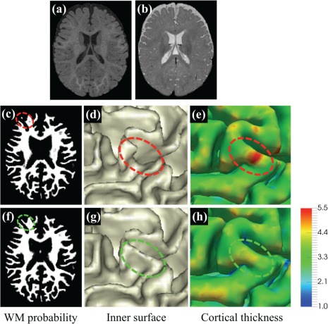
Comparison of LINKS and the proposed method. (a) and (b) show T1‐ and T2‐weighted isointense infant brain images with extremely low tissue contrast. (c) and (f) are the WM probability maps estimated by LINKS (Wang et al., 2015) and the proposed work with anatomical guidance, respectively, with their corresponding inner surfaces shown in (d) and (g). In (d), the region indicated by the red ellipse is topologically correct, but anatomically incorrect due to missing of a gyral region. Corresponding thickness maps shown on the outer surface by LINKS and the proposed work are provided in (e) and (h), respectively [Color figure can be viewed at http://wileyonlinelibrary.com]
Many pioneer works (Anbeek et al., 2008; Cocosco, Zijdenbos, & Evans, 2003; Gui et al., 2012; Isgum et al., 2015; Leroy et al., 2011; Makropoulos et al., 2014; Merisaari et al., 2009; Moeskops et al., 2016; Prastawa, Gilmore, Lin, & Gerig, 2005; Shi et al., 2009; Shi et al., 2011; Shi et al., 2010; Song, Awate, Licht, & Gee, 2007; Wang et al., 2014b; Wang, Shi, Lin, Gilmore, & Shen, 2011; Warfield, Kaus, Jolesz, & Kikinis, 2000; Weisenfeld & Warfield, 2009; Xue et al., 2007; Xue, Shen, & Davatzikos, 2006) have been proposed for brain segmentation and have achieved encouraging results. Recently, a minimal processing pipeline was proposed for neonatal cortical surface reconstruction (Makropoulos et al., 2018). This pipeline consists of tissue segmentation, cortical surface extraction, and cortical surface inflation. However, most of previous work focused on segmentation of neonatal (<3 months of age) brain images with relatively high tissue contrast in T2‐weighted image. Related reviews on neonatal brain MRI segmentation methods can be found in Devi, Chandrasekharan, Sundararaman, and Alex (2015) and Makropoulos, Counsell, and Rueckert (2017). To the best of our knowledge, only few studies focus on the segmentation of 6‐month infant brain images with risk of autism. In 2012, a pioneering work (Hazlett et al., 2012) reported the findings on brain volume in 6–7‐month‐old infants at high familial risk for autism; however, these findings were obtained only on the total brain volume (GM plus WM) measures, without separating GM and WM, due to the challenges in 6‐month brain segmentation. Similarly, a recent work in 2017 (Shen et al., 2017) found increased axial‐CSF in the subarachnoid space for high‐risk infants who later develop autism. In another recent Nature article in 2017 (Hazlett et al., 2017), they employed an indirect way for segmentation of 6‐month images by warping the segmentation from their follow‐up 12‐months/24‐months images. The warping was based on ANTs (Avants et al., 2011) with normalized cross correlation of joint T1‐ and T2‐weighted intensity images. Due to the extremely low contrast of 6‐month images, the longitudinal image correspondences were difficult to identify, which may result in under‐segmented WM and thus thicker cortical thickness. A similar strategy of using follow‐up scans for guiding the segmentation of 6‐month subjects was also employed in Vardhan, Fishbaugh, Vachet, and Gerig (2017). One of the major limitations of these methods (Hazlett et al., 2017; Vardhan et al., 2017) is that they fully depend on the availability of follow‐up 12‐month/24‐month images. Given a new acquired 6‐month MRI scan, the segmentation has to be delayed until 12‐month/24‐month follow‐up scans are acquired, which is not practical. To identify brain biomarkers of autism in the very early stage for early intervention, a standalone method is highly needed.
Recently, a learning‐based multi‐sources integration framework (namely LINKS) (Wang et al., 2015) was proposed to adaptively integrate information from both intensity images and tentatively estimated tissue probability maps for 6‐month infant brain image segmentation. Despite of relatively reasonable results, one major limitation of this method is that the prior anatomical knowledge of the brain is largely ignored during the segmentation. Consequently, the LINKS method cannot guarantee the topological correctness of segmentation results. Indeed, topological errors caused by inaccurate segmentation are frequently seen during cortical surface reconstruction, especially in infant brains (Hao, Li, Wang, Meng, & Shen, 2016). To address these issues, many sophisticated correction methods (Bazin & Pham, 2005; Fischl, Liu, & Dale, 2001; Han et al., 2004; Shattuck & Leahy, 2001; Shi, Lai, Toga, & Initi, 2013) could be used after tissue segmentation. In general, topological correction typically involves two sequential tasks, that is, (a) locating topologically defected regions and (b) correcting them. For example, Hao et al. (2016) proposed an infant‐dedicated topological correction method, which can correct the topologically defected regions by referring to a set of registered topologically correct reference images. Nonetheless, this method is computationally expensive, since it requires conducting multiple nonlinear registrations between the reference images and the to‐be‐corrected image. Moreover, without the prior anatomical knowledge, topological correction cannot necessarily generate desired results (Segonne, Pacheco, & Fischl, 2007). Particularly, due to low contrast between WM and GM in 6‐month infant brain images, WM voxels may be under‐segmented (as shown in Figure 1c), resulting in a “U”‐shape in the inner surface. A typical example can be seen in Figure 1d. The under‐segmented WM usually results in an increased cortical thickness, as shown in Figure 1e. It is worth noting that WM surface indicated in the red ellipse is topologically correct but anatomically incorrect (Yotter, Dahnke, Thompson, & Gaser, 2011). In such a case, correction operation will not be involved since it is already topologically correct.
Therefore, it is highly necessary to incorporate prior anatomical knowledge into tissue segmentation. In this work, we will consider the following two types of anatomical knowledge:
(A1) The human cerebral cortex is a folded sheet of GM wrapping WM;
(A2) Cortical thickness is within a certain range.
Based on the anatomical knowledge, inspired by previous works (Wang et al., 2015; Zeng, Staib, Schultz, & Duncan, 1998; Zikic, Glocker, & Criminisi, 2014), we propose a new anatomy‐guided joint tissue segmentation and topological correction framework for infant brain MRI, by using the above‐mentioned two types of anatomical knowledge. According to the discussions in the previous paragraph and as a concluding remark by the results in Figure 1, we hypothesize that inaccurate segmentation or topological errors will result in abnormal cortical thickness. For example, cortical thickness in the missing gyral region shown in Figure 1e is unexpectedly large. For simplicity, we denote the inner surface as the WM/GM boundary, and the outer surface as the GM/CSF boundary. Based on (A1) and (A2), given an outer (or inner) surface, the location of the inner (or outer) surface can be roughly estimated, which can help recover the missing gyri with unexpectedly large cortical thickness. Since tissue contrast between GM and CSF is much higher than that between GM and WM, it is more feasible to use the outer surface (i.e., GM/CSF boundary) to guide the inner surface estimation. Accordingly, we first train a sequence of classifiers to extract CSF from isointense infant brain images to construct the anatomical guidance. In our implementation, we employ a signed distance map with respect to GM/CSF boundary as the anatomical guidance. With the anatomical guidance, we then train another sequence of classifiers for joint tissue segmentation and topological correction.
2. METHODS
We will first introduce the dataset used in this study. Then we introduce the proposed method to generate the anatomical guidance by classifying the brain images into two classes CSF and WM + GM. Based on the generated anatomical guidance, we further classify each WM + GM map into separate WM and GM maps.
2.1. Dataset and image preprocessing
The T1‐ and T2‐weighted MR images of 50 de‐identified infants were from National Database for Autism Research (NDAR). They were acquired at around 6 months of age on a Siemens 3T scanner. All scans were acquired while the infants were naturally sleeping and fitted with ear protection, with their heads secured in a vacuum‐fixation device. T1‐weighted MR images were acquired with 160 sagittal slices using parameters: TR = 2,400 ms, TE = 3.16 ms and resolution = 1 1 1 mm3. T2‐weighted MR images were obtained with 160 sagittal slices using parameters: TR =3,200 ms, T2 = 499 ms and resolution = 1 × 1 × 1 mm3. Note that the imaging protocol has been optimized to maximize tissue contrast (Hazlett et al., 2012). In case the acquired images were severely affected by motion, the acquisition was repeated until satisfactory images were obtained. For image preprocessing, T2‐weighted images were linearly aligned onto their corresponding T1‐weighted images. Afterward, skull stripping and intensity inhomogeneity correction were performed using in‐house tools (Shi et al., 2012a; Tustison et al., 2010).
Accurate manual segmentation, providing labels for training, is of great importance for learning‐based segmentation methods. Due to low contrast and huge number of voxels in brain images, manual segmentation is time‐consuming (Rodrigues et al., 2015). Hence, to generate reliable manual segmentations, we first take advantage of longitudinal follow‐up 24‐month scans with high tissue contrast to generate an initial automatic segmentation for isointense subjects by using a publicly available software iBEAT (http://www.nitrc.org/projects/ibeat/). This is based on the fact that, at term birth, the major sulci and gyri in the brain are already present, and are generally preserved but only fine‐tuned during early postnatal brain development (Chi, Dooling, & Gilles, 1977). Therefore, we can utilize the longitudinal late‐time‐point images (e.g., 24‐month), which can be segmented with a high accuracy by using existing segmentation tools, for example, FreeSurfer (Fischl, 2012), to guide the segmentation of early‐time‐point (e.g., 6‐month) infant images. Figure 2 shows the automatic segmentation results by iBEAT on four representative subjects. Second, based on the segmentation results by iBEAT, manual editing was further performed by an experienced neuroradiologist. Details of manual protocol are available in the supplement. The corresponding manual segmentation results are shown in the 4th column of Figure 2, with their difference maps compared to iBEAT‐based results shown in the last column. For each subject, it took almost a whole week (40 hr) for manual segmentation, with around 214,801 ± 14,835 voxels (26%±1.8% of total brain volume) re‐labeled. In such a way, the issue of the potential bias from the automatic segmentations can be largely minimized and also the quality of manual segmentation can be ensured. Considering that there are almost 10,000 subjects archived in NDAR, we believe it is worth to make such a great manual annotation effort, which will make our learning algorithm more accurate and robust on this large dataset. Note that these follow‐up scans are used only to generate manual segmentations for training. After training, segmentation will be performed using only 6‐month‐old infant images, without reliance on any follow‐up scans.
Figure 2.
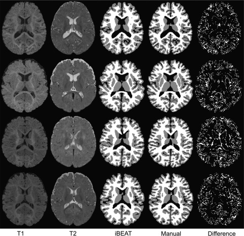
Comparison of segmentations. The 1st and 2nd columns show the original T1‐ and T2‐weighted 6‐month infant brain images, with the automatic segmentation results by iBEAT and the further manual corrections shown in the 3rd and 4th columns. The differences between iBEAT and manual correction results are also provided in the last column
2.2. Anatomical guidance
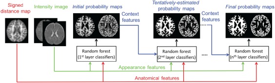
To derive anatomical guidance from the outer surface (i.e., GM/CSF boundary), we need to first classify brain images into two classes, that is, CSF and WM + GM. Many classic methods can be employed for this binary classification problem. Similar to the previous work (Wang et al., 2015), we employ both intensity images and tentatively estimated tissue probability maps to train a sequence of classifiers for CSF versus WM + GM classification. The flowchart is shown in Figure 3, which contains three main components in the training stage. Specifically, (a) we use the appearance features extracted from intensity images, and employ random forests (Breiman, 2001) to train the first‐layer classifiers. (b) Based on the trained first‐layer classifiers, we can derive initial CSF and WM + GM probability maps. Inspired by the auto‐context model (Loog & Ginneken, 2006; Tu & Bai, 2010), we then extract context features from the tentatively estimated tissue probability maps, together with appearance features from intensity images, to train the second‐layer classifiers, for refining the segmentation results. (c) By iteratively training classifiers using both intensity images and the updated tissue probability maps, we can train a sequence of classifiers for segmentation. In the testing stage, the learned classifiers at each layer can be applied sequentially to iteratively refine the estimated probability maps for a new testing image.
Figure 3.
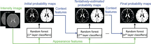
Flowchart of training a sequence of classifiers for CSF versus WM + GM classification [Color figure can be viewed at http://wileyonlinelibrary.com]
Figure 4 shows the finally estimated CSF and WM + GM probability maps for a testing image (the same image in Figure 1). It can be observed that CSF has been reasonably identified, especially for CSF in sulcal regions, which will largely prevent possible topological errors such as handles, in the beginning stage.
Figure 4.
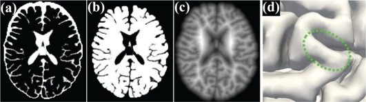
Demonstration of tentative results. (a) and (b) show the estimated CSF and WM + GM probability maps for the testing image in Figure 1. Also, (c) illustrates the signed distance map with respect to the outer surface (d) [Color figure can be viewed at http://wileyonlinelibrary.com]
Based on classification results, it is straightforward to construct a signed distance map (i.e., a level set function) with respect to the boundary of GM/CSF, as shown in Figure 4c. Basically, the function value at each voxel is the shortest distance to its nearest point in the boundary of GM/CSF, and it takes positive values for voxels inside of WM + GM, while negative values outside of WM + GM. Therefore, the zero level set corresponds to the outer surface, as shown in Figure 4d. It is worth noting that the definition of the signed distance map matches the brain anatomical knowledge: (a) the sign will roughly constrain WM to be inside of WM + GM (A1); and (b) the absolute distance value will further relatively and precisely constrain WM to keep the cortical thickness within a reasonable range (A2).
2.3. Anatomy‐guided tissue segmentation and topological correction
Similar to the method in Section 2.2, we further classify each WM + GM map into separate WM and GM maps by training another sequence of classifiers. It is worth noting that, besides using intensity images and tentatively estimated tissue probabilities maps, the signed distance maps (used as anatomical guidance) will also be incorporated into the learning process. The flowchart for classifying WM and GM is shown in Figure 5. Specifically, in the training stage, (a) we train the first‐layer of classifiers by extracting appearance features from intensity images along with the anatomical features from the signed distance map. (b) Based on the trained first‐layer classifiers, we can derive initial WM and GM probability maps. Then, we will extract context features from the estimated tissue probability maps, together with appearance features from intensity images and also anatomical features from the signed distance map, to train the second‐layer classifiers. (c) By iteratively training classifiers with random forests on the intensity images, the signed distance map and the updated tissue probability maps, we can train a sequence of classifiers for classification. Note that, in our learning‐based framework, the spatially varying cortical thickness (Fischl, 2012; Li et al., 2014a) is implicitly and adaptively learned from the training images, instead of being explicitly defined in a constant range as in Zeng et al. (1998).
Figure 5.
Flowchart of training a sequence of classifiers for WM versus GM classification [Color figure can be viewed at http://wileyonlinelibrary.com]
In the testing stage, the learned classifiers are sequentially applied on each testing image to iteratively refine the estimated probability maps, steered by the anatomical guidance constructed in Section 2.2. Figure 6 shows an example with the tentatively estimated WM probability maps and the corresponding inner cortical surfaces (from left to right) estimated by the trained classifiers for the testing image illustrated in Figure 1. Recall the missing gyral region in the inner cortical surface of Figure 1, which leads to unexpectedly large cortical thickness. With the anatomical guidance from the outer surface in the last column of Figure 6 (copied from Figure 4d), as indicated by the green ellipse, more WM voxels are expected to keep cortical thickness within a reasonable range. It can be observed that the WM probability in the green ellipse is gradually enhanced, and thus the missing gyrus is gradually recovered by the anatomical guidance, along which the cortical thickness (in the last row) is becoming reasonable. Similarly, the topological errors, for example, holes or handles, causing abnormal cortical thickness, can also be corrected, with the results shown in the following section (see Figure 7).
Figure 6.
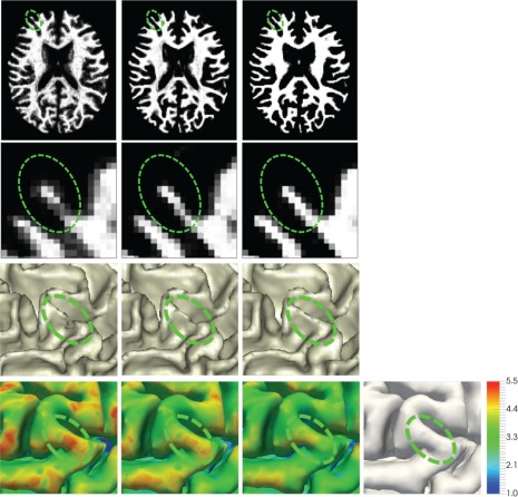
The first two rows (from left to right) show the tentatively estimated WM probability maps and their zoomed views estimated by a sequence of classifiers, with the inner surface and also the cortical thickness maps on the outer surfaces shown in the last two rows, for the testing image in Figure 1. Steered by the anatomical guidance from the outer surface as shown in the last column (copied from Figure 4d), the missing gyrus can be gradually recovered [Color figure can be viewed at http://wileyonlinelibrary.com]
Figure 7.
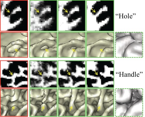
Importance of using the anatomical guidance to correct topological errors. The 1st column shows the WM probabilities and their corresponding inner surfaces estimated without using anatomical guidance. The 2nd to 4th columns show the tentatively estimated results of the proposed method. Steered by the anatomical guidance from the last column, the errors are gradually corrected [Color figure can be viewed at http://wileyonlinelibrary.com]
2.4. Implementation: Feature extraction, classifier training and testing
For training the classifiers, we can extract various features from intensity images, tissue probability maps and signed distance maps, such as SIFT (Lowe, 1999), HOG (Dalal & Triggs, 2005), and LBP features (Ahonen, Hadid, & Pietikainen, 2006). In this work, although other kinds of features could also be used, we use 3D Haar‐like features (Viola & Jones, 2004) mainly due to their computational efficiency. Specifically, for each voxel , its Haar‐like features are computed as the local mean intensity of any randomly displaced cubical region or the mean intensity difference between any two randomly displaced, asymmetric cubical regions ( and ), within the image patch (Han, 2013):
| (1) |
where is the patch centered at voxel , is any kind of image types (intensity images, tissue probability maps, or signed distance maps), and the parameter indicates whether one or two cubical regions are used. In the intensity image, its intensities are normalized to have the unit norm (Cheng, Liu, & Yang, 2009; Wright et al., 2010). However, as the probability maps are already in the range [0 1], there is no need to conduct any further normalization on them; similarly, for the patches from signed distance maps, we do not perform any normalization to preserve the physical meanings they bear. In theory, for each voxel, we are able to determine an infinite number of such features. For simplicity, we extract 3D Haar‐like features from intensity images, tissue probability maps and signed distance maps as appearance, context and anatomical features, respectively.
Based on the extracted features , we will use random forest as classifier to determine a class label for a given testing voxel . The random forest is an ensemble of decision trees, indexed by , where is the total number of trees at each layer. To inject the randomness for improved generalization (Criminisi, Shotton, & Konukoglu, 2011), only a subset of features and training voxels are selected for training each decision tree. During training, each decision tree will learn a weak class predictor . Specifically, a decision tree consists of two types of nodes, namely internal nodes (nonleaf nodes) and leaf nodes. Each internal node stores a split (or decision) function to divide the training data to its left or right child node based on one feature and its threshold, which are learned to maximize the information gain of spitted training data. On the other hand, each leaf stores the final answer (predictor) (Criminisi et al., 2011). We commence by constructing its root (internal) node, where its split function is optimized to split the training samples into two subsets, which are then placed in the left and right children (internal) nodes. The tree continues growing as more splits are made, and stops at a specified depth , or when satisfying the condition that a leaf node contains less than a certain number of training samples ( ). Finally, by simply counting the labels of all training samples, which reach each leaf node, we can associate each leaf node with the empirical distribution over classes .
During testing, each voxel to be classified is independently pushed through each trained tree , by applying the learned split functions. Upon arriving at a leaf node , the empirical distribution of the leaf node is used to determine the class probability of the testing sample at tree , that is, . The final probability of the testing sample is computed as the average of the class probabilities from individual trees, that is, .
In our implementation, for each tissue type, we randomly select 5,000 training voxels from each training subject. Then, for each training voxel with the patch size of 7 × 7 × 7, 10,000 random Haar‐like features are equally extracted from T1‐ and T2‐weighted MR images, tentatively estimated tissue probability maps of WM, GM, and CSF, and signed distance maps. In each layer of classifier training, we train =20 decision trees. We conservatively stop the growth of tree at a depth of =100, with a minimum of = 8 samples for each leaf node. These parameters for classifier training were empirically set according to Wang et al. (2015) (Please refer to Section 2.2 for the discussion on parameter selection).
3. EXPERIMENTAL RESULTS
We have validated the proposed method on 50 6‐month infant subjects using 5‐fold cross‐validation with five repeats. We first demonstrate the effectiveness to correct topological errors and the robustness to motion, and then perform comparisons with state‐of‐the‐art methods. For evaluation, visual inspection is employed for qualitative comparison, and the manual segmentation is considered as the “ground truth” for quantitative comparison (see Section 2.1).
3.1. Quantitative evaluation metrics
We mainly employ Dice ratio (DR) to evaluate the segmentation accuracy, which is defined as:
| (2) |
where and are the two segmentation results of the same image. We also evaluate the accuracy by measuring the modified Hausdorff distance (MHD), which is defined as the 95th‐percentile Hausdorff distance:
| (3) |
where is the surface of segmentation , represents the ranked distance such that , and is the nearest Euclidean distance from a surface point to the surface .
3.2. Topological correction
In Figure 6, we have shown the advantage of using the anatomical knowledge in guiding tissue segmentation. In Figure 7, we further demonstrate the effectiveness of the anatomical guidance for topological correction. The 1st column in Figure 7 shows the results without anatomical guidance, causing holes and handles. These holes and handles result in abnormal cortical thickness. The 2nd to 4th columns show the tentatively estimated WM probability maps and the corresponding inner surfaces, steered by the anatomical guidance shown in the last column. It can be observed that these topological errors are gradually corrected by using the anatomical guidance.
3.3. Robustness to motion
During the image acquisition process, motion from infants is inevitable. We have to repeat the acquisition in case the acquired images were seriously affected by infant motion. However, there may still exist some small motion. Therefore, a motion‐robust segmentation method is highly desired. Figure 8 shows an example of T1‐ and T2‐weighted images with motion effects. Existing work without considering anatomical knowledge, such as LINKS (Wang et al., 2015) and topological correction (TC) method (Hao et al., 2016), cannot achieve reasonable results, as shown in (a) and (b), respectively. By contrast, the proposed work is robust to the motion and thus produces the relatively reasonable result (c), steered by anatomical guidance.
Figure 8.
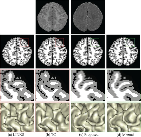
Comparisons with learning‐based segmentation method (LINKS) (Wang et al., 2015) and topological correction (TC) method (Hao et al., 2016) on a subject with motion. The 1st row shows T1‐ and T2‐weighted images with motion effects. Without anatomical guidance, LINKS (a) and TC (b) are sensitive to motion effect. By contrast, our proposed anatomy‐guided framework achieves reasonable results (c) [Color figure can be viewed at http://wileyonlinelibrary.com]
3.4. Comparison with the state‐of‐the‐art methods
In the following, we quantitatively compare our method mainly with LINKS (Wang et al., 2015) on 50 6‐month infant subjects, since LINKS achieves the state‐of‐the‐art segmentation results. We will also compare with the infant‐dedicated topological correction (TC) method (Hao et al., 2016). Figure 9 demonstrates the segmentation results of different methods for a typical subject. The 1st row shows the original T1‐ and T2‐weighted images and their corresponding anatomical guidance from zero level set function (i.e., the outer cortical surface). The 2nd and 4th rows show the segmentation results and the inner cortical surfaces obtained by the different methods, with their corresponding zoomed views also shown in the 3rd and 5th rows, respectively. We first visually compare the proposed method with LINKS, which also effectively trains a sequence of classifiers on intensity images and tentatively estimated tissue probability maps. However, without anatomical guidance, some WM are missing in the results of LINKS, due to the extremely low tissue contrast between WM and GM, and also there are many topological errors in the reconstructed inner cortical surface. To correct those topological errors, we further employ a learning‐based topological correction (Hao et al., 2016) to refine the results as shown in the 2nd column of Figure 9. However, due to large segmentation and topological errors, the registered reference images could not be aligned well with the to‐be‐corrected image. Consequently, the holes are incorrectly broken, which are actually topologically correct but anatomically incorrect, especially for the missing gyrus. In contrast, our proposed anatomy‐guided framework achieves better results, with appropriately recovered gyrus and also anatomically corrected holes/handles.
Figure 9.
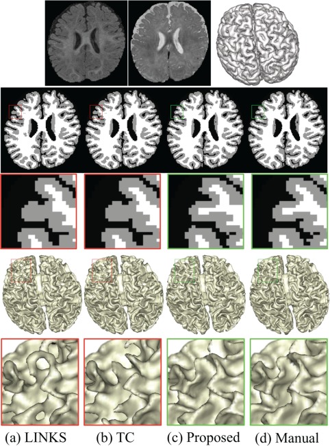
Comparisons with the learning‐based segmentation method (LINKS) (Wang et al., 2015) and the topological correction (TC) method (Hao et al., 2016). The 1st row shows T1‐, T2‐weighted images, and anatomical guidance from zero level set function (i.e., the outer cortical surface). Without anatomical guidance, the results by LINKS have topological errors in the reconstructed inner cortical surface (a). Topological correction results by Hao et al. (2016) are still anatomically incorrect (b). By contrast, our proposed anatomy‐guided framework achieves better results (c), with appropriately recovered gyri and also corrected holes/handles [Color figure can be viewed at http://wileyonlinelibrary.com]
Furthermore, we quantitatively compare our method with LINKS and TC via both DR and the MHD, with the results given in Table 1. To investigate whether the segmentation results achieved by our method are significantly different from those obtained by each competing method, we further perform a paired t‐test on both DR and MHD. It can be seen from Table 1 that our proposed method achieves more accurate results in terms of both DR and MHD. It is worth noting that DR of CSF is higher than that of WM or GM in all three methods, which is mainly due to the relatively high contrast between CSF and other tissues. That is also the reason that we use the outer surface (i.e., GM/CSF boundary) to guide the inner surface estimation.
Table 1.
Averaged Dice ratio (in percentage) and MHD (in mm) for three different methods on 50 isointense infant images
| Method | LINKS (Wang et al., 2015) | TC (Hao et al., 2016) | Proposed | |
|---|---|---|---|---|
| Dice Ratio | WM | 87.1 ± 0.56 (p=0.0001) | 87.5 ± 0.45 (p=0.0001) | 89.4 ± 0.31 |
| GM | 86.5 ± 0.78 (p=0.0003) | 87.2 ± 0.63 (p=0.0003) | 90.5 ± 0.55 | |
| CSF | 92.6 ± 0.29* (p=0.90) | 92.6 ± 0.29* (p=0.90) | 92.5 ± 0.31 | |
| MHD (in mm) | WM/GM | 1.50 ± 0.37 (p=0.0001) | 1.29 ± 0.25 (p=0.0001) | 0.89 ± 0.11 |
The bold indicates that the respective result is significantly better than others (p value < .005). The symbol * in the table indicates that the topological correction (TC) only corrects the inner cortical surface, and thus its accuracy on CSF segmentation is the same as the original LINKS (Wang et al., 2015).
To further demonstrate the improvement by the proposed method, in Figure 10, we present a representative comparison between different methods with the error maps. As shown in the center of Figure 10, the blue indicates over‐segmentation (e.g., handles) and the green indicates under‐segmentation (e.g., missing U‐gyral patterns and holes). Note that we have excluded these isolated error regions, each with the total volume smaller than five voxels. In the surrounding of Figure 10, the zoomed views of one handle, one hole and two missing U‐gyral patterns are also presented for a better visualization. The quantitative measurement of segmentation errors with respect to volume is listed in Table 2. From the table, we find the under‐segmentation (e.g., missing U‐gyral patterns) denominate the errors by the LINKS and TC. These segmentation errors, for example, holes, handles and missing U‐gyral patterns, causing abnormal cortical thickness, have been largely corrected by the proposed work with the anatomy guidance.
Figure 10.
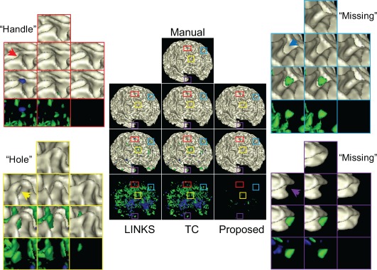
Comparison between different methods. Center: the 1st row shows the gold standard result and the 2nd row shows the results by LINKS, TC and the proposed method. The 3rd row show differences between the 1st and 2nd rows, with the blue indicating over‐segmentation (e.g., handles), the green indicating under‐segmentation (e.g., missing U‐gyral patterns and holes), while the beige indicating consistence with the gold standard result. The 4th row shows only error regions. Surrounding: the zoomed views of one handle, one hole and two missing U‐gyral patterns, indicated by arrows, are also presented for better visualization [Color figure can be viewed at http://wileyonlinelibrary.com]
Table 2.
Segmentation errors (in voxel) for different methods on 50 isointense infant images
3.5. Estimation of cortical thickness
As introduced in Section 1, accurate segmentation is critically important to characterize brain measurements, for example, cortical thickness. We further applied the proposed work on 127 infant subjects at around 6‐month of age from NDAR and calculated the cortical thickness. The mean cortical thickness over 127 infant subjects is 2.689 ± 0.092 mm, which is in line with the previous studies (Fischl & Dale, 2000; Geng et al., 2017; Li, Lin, Gilmore, & Shen, 2015; Lyall et al., 2015). For example, reported cortical thickness from post‐mortem adult brains is in the range of 1.3–4.5 mm (Henery & Mayhew, 1989), with the mean thickness of 2.5 ± 0.7 mm (Fischl & Dale, 2000). In Li et al. (2014a), the mean cortical thickness for 13 infant subjects is 2.611 ± 0.080 mm at 6 months of age. However, it might be interesting to note that the mean cortical thickness reported in a recent study (Hazlett et al., 2017) for 42 6‐month infant subjects is 5.971 ± 0.255 mm, which is much higher than previous studies. Methodological differences could potentially account for these conflicting findings. In (Hazlett et al., 2017), the cortical surfaces at 6‐month subjects were determined by warping the cortical surfaces from their follow‐up 12‐month/24‐month subjects based on ANTs (Avants et al., 2011) with normalized cross correlation of joint T1‐ and T2‐weighted images. Due to the extremely low contrast of 6‐month images, the cortical correspondences were difficult to identify, which may result in under‐segmented WM and thus thicker cortical thickness.
4. DISCUSSIONS AND CONCLUSION
In this article, we proposed a novel anatomy‐guided framework for joint tissue segmentation and topological correction for 6‐month infant MRI, which is characterized with extremely low contrast between GM and WM caused by the inherent ongoing WM myelination and maturation. We took advantage of relatively high contrast between GM and CSF to construct the anatomical guidance to guide the segmentation. The experimental results have demonstrated that the anatomical guidance is of great importance for tissue segmentation of infant brain MRI. Although the proposed method still cannot guarantee the topological correctness, the topological errors are largely reduced as demonstrated by experimental results.
There are many quantitative parameters, such as cortical thickness, surface area, gyrification and curvature, to measure early brain development. In this work, we have estimated cortical thickness based on accurate segmentation results. It is defined as the minimal distance between the inner surface and outer surface. Therefore, given a voxel with a resolution of 1 × 1 × 1 mm3, one voxel error will result in ±1 mm thickness estimation error. Therefore, thickness is much more sensitive with respect to the segmentation accuracy, compared with surface area, gyrification and volume, especially considering the fact that the mean thickness is ∼2.5 mm (Fischl & Dale, 2000; Geng et al., 2017; Li et al., 2015; Lyall et al., 2015). As an example, in Section 3.5, due to possible under‐segmented WM, the mean cortical thickness reported in Hazlett et al. (2017) for 42 6‐month infant subjects is 5.971 ± 0.255 mm, which is much higher than those reported in the previous studies (Fischl & Dale, 2000; Geng et al., 2017; Li et al., 2015; Lyall et al., 2015).
There are many discriminative classification algorithms such as support vector machines (SVM) (Burges, 1998), which have been applied successfully to many tasks. However, compared with SVM, random forests have two major advantages. (a) Random forests are inherently multi‐label classifiers, which allows us to classify different tissues simultaneously. By contrast, SVMs are inherently binary classifiers. In order to classify different tissues, they are often applied hierarchically or in an one‐versus‐all manner. As also confirmed in works (Bosch, Zisserman, & Muoz, 2007; Pei, Criminisi, Winn, & Essa, 2007), random forests have also shown to be better suited to multi‐class problems than SVMs. (b) Random forests are invariant with scales/ranges of different types of features, while, for SVM, the contribution weights of different types of features have to be carefully tuned (Hastie, Tibshirani, & Friedman, 2001). For example, in our case, the scale of probability maps is in [0 1], while the scale of signed distance maps is in [−40 20]. If we use SVM, we have to carefully consider the contribution of each type of features. In our work, the parameters for training the random forests were empirically set according to Wang et al. (2015). Generally, for the number of trees, we found that the more the better, but also the longer it will take to do the training. Hence, we made a trade‐off between the performance and running time, and set it to 20. Regarding the allowed depth of trees, in general, a low depth will be likely to under‐fitting, while a high value will be likely to over‐fitting. The optimal patch size is related to the complexity of the anatomical structure (Coupé et al., 2011; Tong, Wolz, Coupé, Hajnal, & Rueckert, 2013). Too small or too large patch size will result in poor performance. In this article, we selected the patch size as 7 × 7 × 7 for the 6‐month infant subjects with the voxel size of 1 × 1 × 1 mm3, according to (Wang et al., 2015).
While the proposed framework produces decent segmentation results compared with previous works, some limitations should be noted. First, we only consider (A1) and (A2) as anatomical knowledge to guide the segmentation. In fact, other anatomical knowledge, for example, gyral convexity and sulcal concavity, can also be potentially employed for further improving the segmentation performance of our proposed method. Second, we extract the same feature type, that is, 3D Haar‐like feature, from both T1‐ and T2‐weighted images, tissue probability maps, and signed distance maps, which may not be the optimal choice. It would be interesting to extract different discriminative features from different types of images, which is one of our future works. Alternatively, instead of designing these hand‐crafted features, we will also consider using deep learning (LeCun, Bengio, & Hinton, 2015) to automatically learn effective feature hierarchies from the infant data. Our future work will also include applying the proposed work on almost 10,000 subjects from NDAR to characterize early brain development and identify possible biomarkers.
Manual labels are critically important for learning‐based methods. Considering the huge amount of manual labeling work, we will share these manual labels with the community, as we did in a MICCAI Grand Challenge (http://iseg2017.web.unc.edu). In this challenge, we have shared manual labels on 10 infant subjects chosen from the pilot study of Baby Connectome Project (BCP), which is recently started and will acquire and publicly release MRI data from 500 typically developing children, ages 0–5 years, over the course of four years. Since we are the organizers of this challenge, we were requested by MICCAI not to participate in this challenge.
Supporting information
Additional Supporting Information may be found online in the supporting information tab for this article.
Supplemental_Figure 1
ACKNOWLEDGMENTS
Data used in the preparation of this manuscript were obtained from the NIH‐supported National Database for Autism Research (NDAR). NDAR is a collaborative informatics system created by the National Institutes of Health to provide a national resource to support and accelerate research in autism. This paper reflects the views of the authors and may not reflect the opinions or views of the NIH or of the Submitters submitting original data to NDAR. This work was supported in part by National Institutes of Health grants MH109773, MH100217, MH070890, EB006733, EB008374, EB009634, AG041721, AG042599, MH088520, MH108914, and MH107815.
Wang L, Li G, Adeli E, et al. Anatomy‐guided joint tissue segmentation and topological correction for 6‐month infant brain MRI with risk of autism. Hum Brain Mapp. 2018;39:2609–2623. 10.1002/hbm.24027
Funding information National Institutes of Health, Grant/Award Numbers: MH109773, MH100217, MH070890, EB006733, EB008374, EB009634, AG041721, AG042599, MH088520, MH108914, and MH107815
REFERENCES
- Ahonen, T. , Hadid, A. , & Pietikainen, M. (2006). Face description with local binary patterns: application to face recognition. IEEE Transactions on Pattern Analysis and Machine Intelligence, 28(12), 2037–2041. [DOI] [PubMed] [Google Scholar]
- Anbeek, P. , Vincken, K. , Groenendaal, F. , Koeman, A. , VAN Osch, M. , & VAN DER Grond, J. (2008). Probabilistic brain tissue segmentation in neonatal magnetic resonance imaging. Pediatric Research, 63(2), 158–163. [DOI] [PubMed] [Google Scholar]
- Avants, B. B. , Tustison, N. J. , Song, G. , Cook, P. A. , Klein, A. , & Gee, J. C. (2011). A reproducible evaluation of ANTs similarity metric performance in brain image registration. Neuroimage, 54(3), 2033–2044. [DOI] [PMC free article] [PubMed] [Google Scholar]
- Bazin, P‐L. , & Pham, D. L. (2005). Topology preserving tissue classification with fast marching and topology templates. IPMI, 19, 234–245. [DOI] [PubMed] [Google Scholar]
- Bosch, A. , Zisserman, A. , & Muoz, X. (2007). Image classification using random forests and ferns. In IEEE 11th international conference on computer vision, 2007 ICCV 2007 (pp. 1–8).
- Breiman, L. (2001). Random forests. Machine Learning, 45(1), 5–32. [Google Scholar]
- Burges, C. C. (1998). A tutorial on support vector machines for pattern recognition. Data Mining and Knowledge Discovery, 2, 121–167. [Google Scholar]
- Cheng, H. , Liu, Z. , & Yang, L. (2009). Sparsity induced similarity measure for label propagation. In IEEE 12th international conference on computer vision, 2009 (pp. 317–324).
- Chi, J. , Dooling, E. , & Gilles, F. (1977). Gyral development of the human brain. Annals of Neurology, 1(1), 86–93. [DOI] [PubMed] [Google Scholar]
- Cocosco, C. A. , Zijdenbos, A. P. , & Evans, A. C. (2003). A fully automatic and robust brain MRI tissue classification method. Medical Image Analysis, 7, 513–527. [DOI] [PubMed] [Google Scholar]
- Coupé, P. , Manjón, J. , Fonov, V. , Pruessner, J. , Robles, M. , & Collins, D. L. (2011). Patch‐based segmentation using expert priors: Application to hippocampus and ventricle segmentation. Neuroimage, 54(2), 940–954. [DOI] [PubMed] [Google Scholar]
- Criminisi, A. , Shotton, J. , & Konukoglu, E. (2011). Decision forests: A unified framework for classification, regression, density estimation, manifold learning and semi‐supervised learning. Foundations and Trends® in Computer Graphics and Vision, 7(2–3), 81–227. [Google Scholar]
- Dalal, N. , & Triggs, B. (2005). Histograms of oriented gradients for human detection. In IEEE computer society conference on computer vision and pattern recognition, 2005 (pp. 886–893, vol. 881). CVPR 2005.
- Damiano, C. R. , Mazefsky, C. A. , White, S. W. , & Dichter, G. S. (2014). Future directions for research in autism spectrum disorders. Journal of Clinical Child and Adolescent Psychology, 43(5), 828–843. [DOI] [PMC free article] [PubMed] [Google Scholar]
- Devi, C. N. , Chandrasekharan, A. , Sundararaman, V. K. , & Alex, Z. C. (2015). Neonatal brain MRI segmentation: A review. Computers in Biology and Medicine, 64, 163–178. [DOI] [PubMed] [Google Scholar]
- Fischl, B. (2012). FreeSurfer. NeuroImage, 62(2), 774–781. [DOI] [PMC free article] [PubMed] [Google Scholar]
- Fischl, B. , & Dale, A. M. (2000). Measuring the thickness of the human cerebral cortex from magnetic resonance images. Proceedings of the National Academy of Sciences of the United States of America, 97(20), 11050–11055. [DOI] [PMC free article] [PubMed] [Google Scholar]
- Fischl, B. , Liu, A. , & Dale, A. M. (2001). Automated manifold surgery: constructing geometrically accurate and topologically correct models of the human cerebral cortex. IEEE Transactions on Medical Imaging, 20(1), 70–80. [DOI] [PubMed] [Google Scholar]
- Gao, W. , Gilmore, J. H. , Shen, D. G. , Smith, J. K. , Zhu, H. T. , & Lin, W. L. (2013). The synchronization within and interaction between the default and dorsal attention networks in early infancy. Cerebral Cortex, 23(3), 594–603. [DOI] [PMC free article] [PubMed] [Google Scholar]
- Geng, X. , Li, G. , Lu, Z. , Gao, W. , Wang, L. , Shen, D. , … Gilmore, J. H. (2017). Structural and maturational covariance in early childhood brain development. Cerebral Cortex, 27, 1795–1807. [DOI] [PMC free article] [PubMed] [Google Scholar]
- Gui, L. , Lisowski, R. , Faundez, T. , Hüppi, P. S. , Lazeyras, F. O. , & Kocher, M. (2012). Morphology‐driven automatic segmentation of MR images of the neonatal brain. Medical Image Analysis, 16(8), 1565–1579. [DOI] [PubMed] [Google Scholar]
- Guze, S. B. (1995). Diagnostic and statistical manual of mental‐disorders, 4th Edition (Dsm‐Iv) ‐ Amer‐Psychiat‐Assoc. American Journal of Psychiatry, 152(8), 1228–1228. [Google Scholar]
- Han, X. (2013). Learning‐boosted label fusion for multi‐atlas auto‐segmentation In Wu G., Zhang D., Shen D., Yan P., Suzuki K., & Wang F. (Eds.), Machine learning in medical imaging (pp. 17–24). Cham: Springer International Publishing. [Google Scholar]
- Han, X. , Pham, D. L. , Tosun, D. , Rettmann, M. E. , Xu, C. , & Prince, J. L. (2004). CRUISE: Cortical reconstruction using implicit surface evolution. Neuroimage, 23(3), 997–1012. [DOI] [PubMed] [Google Scholar]
- Hao, S. , Li, G. , Wang, L. , Meng, Y. , & Shen, D. (2016). Learning‐based topological correction for infant cortical surfaces. In MICCAI (pp. 219–227). Cham: Springer. [DOI] [PMC free article] [PubMed]
- Hastie, T. , Tibshirani, R. , & Friedman, J. H. (2001). The elements of statistical learning: Data mining, inference, and prediction: with 200 full‐color illustrations. New York: Springer. [Google Scholar]
- Hazlett, H. C. , Gu, H. , McKinstry, R. C. , Shaw, D. W. W. , Botteron, K. N. , Dager, S. , … IBIS Network . (2012). Brain volume findings in six month old infants at high familial risk for autism. The American Journal of Psychiatry, 169, 601–608. [DOI] [PMC free article] [PubMed] [Google Scholar]
- Hazlett, H. C. , Gu, H. B. , Munsell, B. C. , Kim, S. H. , Styner, M. , Wolff, J. J. , … IBIS Network . (2017). Early brain development in infants at high risk for autism spectrum disorder. Nature, 542(7641), 348–351. [DOI] [PMC free article] [PubMed] [Google Scholar]
- Henery, C. C. , & Mayhew, T. M. (1989). The cerebrum and cerebellum of the fixed human‐brain ‐ efficient and unbiased estimates of volumes and cortical surface‐areas. Journal of Anatomy, 167, 167–180. [PMC free article] [PubMed] [Google Scholar]
- Isgum, I. , Benders, M. J. N. L. , Avants, B. , Cardoso, M. J. , Counsell, S. J. , Gomez, E. F. , … Viergever, M. A. (2015). Evaluation of automatic neonatal brain segmentation algorithms: The NeoBrainS12 challenge. Medical Image Analysis, 20, 135–151. [DOI] [PubMed] [Google Scholar]
- LeCun, Y. , Bengio, Y. , & Hinton, G. (2015). Deep learning. Nature, 521(7553), 436–444. [DOI] [PubMed] [Google Scholar]
- Leroy, F. , Mangin, J. , Rousseau, F. , Glasel, H. , Hertz‐Pannier, L. , Dubois, J. , & Dehaene‐Lambertz, G. (2011). Atlas‐free surface reconstruction of the cortical grey‐white interface in infants. PLoS One, 6(11), e27128. [DOI] [PMC free article] [PubMed] [Google Scholar]
- Li, G. , Lin, W. , Gilmore, J. H. , & Shen, D. (2015). Spatial patterns, longitudinal development, and hemispheric asymmetries of cortical thickness in infants from birth to 2 years of age. The Journal of Neuroscience, 35(24), 9150–9162. [DOI] [PMC free article] [PubMed] [Google Scholar]
- Li, G. , Nie, J. X. , Wang, L. , Shi, F. , Gilmore, J. H. , Lin, W. L. , & Shen, D. G. (2014a). Measuring the dynamic longitudinal cortex development in infants by reconstruction of temporally consistent cortical surfaces. Neuroimage, 90, 266–279. [DOI] [PMC free article] [PubMed] [Google Scholar]
- Li, G. , Wang, L. , Shi, F. , Lyall, A. E. , Ahn, M. , Peng, Z. W. , … Shen, D. G. (2016). Cortical thickness and surface area in neonates at high risk for schizophrenia. Brain Structure & Function, 221(1), 447–461. [DOI] [PMC free article] [PubMed] [Google Scholar]
- Li, G. , Wang, L. , Shi, F. , Lyall, A. E. , Lin, W. L. , Gilmore, J. H. , & Shen, D. G. (2014b). Mapping longitudinal development of local cortical gyrification in infants from birth to 2 years of age. Journal of Neuroscience, 34, 4228–4238. [DOI] [PMC free article] [PubMed] [Google Scholar]
- Loog, M. , & Ginneken, B. (2006). Segmentation of the posterior ribs in chest radiographs using iterated contextual pixel classification. IEEE Transactions on Medical Imaging, 25(5), 602–611. [DOI] [PubMed] [Google Scholar]
- Lowe, D. G. (1999). Object recognition from local scale‐invariant features. In The proceedings of the seventh ieee international conference on computer vision, 1999 (vol. 1152, pp. 1150–1157).
- Lyall, A. E. , Shi, F. , Geng, X. , Woolson, S. , Li, G. , Wang, L. , … Gilmore, J. H. (2015). Dynamic development of regional cortical thickness and surface area in early childhood. Cerebral Cortex, 25(8), 2204–2212. [DOI] [PMC free article] [PubMed] [Google Scholar]
- Makropoulos, A. , Aljabar, P. , Wright, R. , Huning, B. , Merchant, N. , Arichi, T. , … Rueckert, D. (2016). Regional growth and atlasing of the developing human brain. Neuroimage, 125, 456–478. [DOI] [PMC free article] [PubMed] [Google Scholar]
- Makropoulos, A. , Counsell, S. J. , & Rueckert, D. (2017). A review on automatic fetal and neonatal brain MRI segmentation. Neuroimage. In press, 10.1016/j.neuroimage.2017.06.074i [DOI] [PubMed] [Google Scholar]
- Makropoulos, A. , Gousias, I. S. , Ledig, C. , Aljabar, P. , Serag, A. , Hajnal, J. V. , … Rueckert, D. (2014). Automatic whole brain MRI segmentation of the developing neonatal brain. IEEE Transactions on Medical Imaging, 33(9), 1818–1831. [DOI] [PubMed] [Google Scholar]
- Makropoulos, A. , Robinson, E. C. , Schuh, A. , Wright, R. , Fitzgibbon, S. , Bozek, J. , … Rueckert, D. (2018). The developing human connectome project: A minimal processing pipeline for neonatal cortical surface reconstruction. Neuroimage, 173, 88–112. [DOI] [PMC free article] [PubMed] [Google Scholar]
- Merisaari, H. , Parkkola, R. , Alhoniemi, E. , Teräs, M. , Lehtonen, L. , Haataja, L. , … Nevalainen, O. S. (2009). Gaussian mixture model‐based segmentation of MR images taken from premature infant brains. Journal of Neuroscience Methods, 182(1), 110–122. [DOI] [PubMed] [Google Scholar]
- Moeskops, P. , Viergever, M. A. , Mendrik, A. M. , de Vries, L. S. , Benders, M. J. N. L. , & Isgum, I. (2016). Automatic segmentation of MR brain images with a convolutional neural network. IEEE Transactions on Medical Imaging, 35(5), 1252–1261. [DOI] [PubMed] [Google Scholar]
- Mostapha, M. , Casanova, M. F. , Gimel'farb, G. , & El‐Baz, A. (2015). Towards non‐invasive image‐based early diagnosis of autism. Medical Image Computing and Computer‐Assisted Intervention ‐ Miccai, 2015(Pt Ii 9350), 160–168. [Google Scholar]
- Paus, T. , Collins, D. L. , Evans, A. C. , Leonard, G. , Pike, B. , & Zijdenbos, A. (2001). Maturation of white matter in the human brain: A review of magnetic resonance studies. Brain Research Bulletin, 54(3), 255–266. [DOI] [PubMed] [Google Scholar]
- Pei, Y. , Criminisi, A. , Winn, J. , & Essa, I. (2007). Tree‐based classifiers for bilayer video segmentation. In IEEE conference on computer vision and pattern recognition, 2007 CVPR '07 (pp. 1–8).
- Prastawa, M. , Gilmore, J. H. , Lin, W. , & Gerig, G. (2005). Automatic segmentation of MR images of the developing newborn brain. Medical Image Analysis, 9(5), 457–466. [DOI] [PubMed] [Google Scholar]
- Qiu, A. Q. , Tuan, T. A. , Ong, M. L. , Li, Y. , Chen, H. , Rifkin‐Graboi, A. , … Meaney, M. J. (2015). COMT haplotypes modulate associations of antenatal maternal anxiety and neonatal cortical morphology. American Journal of Psychiatry, 172, 163–172. [DOI] [PubMed] [Google Scholar]
- Rodrigues, K. D. , Ben‐Avi, E. , Sliva, D. D. , Choe, M. S. , Drottar, M. , Wang, R. P. , … Zollei, L. (2015). A FreeSurfer‐compliant consistent manual segmentation of infant brains spanning the 0–2 year age range. Frontiers in Human Neuroscience, 9, 21. [DOI] [PMC free article] [PubMed] [Google Scholar]
- Segonne, F. , Pacheco, J. , & Fischl, B. (2007). Geometrically accurate topology‐correction of cortical surfaces using nonseparating loops. IEEE Transactions on Medical Imaging, 26(4), 518–529. [DOI] [PubMed] [Google Scholar]
- Shattuck, D. W. , & Leahy, R. M. (2001). Automated graph‐based analysis and correction of cortical volume topology. IEEE Transactions on Medical Imaging, 20(11), 1167–1177. [DOI] [PubMed] [Google Scholar]
- Shen, M. D. , Kim, S. H. , McKinstry, R. C. , Gu, H. , Hazlett, H. C. , Nordahl, C. W. , … IBIS Network . (2017). Increased extra‐axial cerebrospinal fluid in high‐risk infants who later develop autism. Biological Psychiatry, 82(3), 186–193. [DOI] [PMC free article] [PubMed] [Google Scholar]
- Shen, M. D. , Nordahl, C. W. , Young, G. S. , Wootton‐Gorges, S. L. , Lee, A. , Liston, S. E. , … Amaral, D. G. (2013). Early brain enlargement and elevated extra‐axial fluid in infants who develop autism spectrum disorder. Brain, 136(9), 2825–2835. [DOI] [PMC free article] [PubMed] [Google Scholar]
- Shi, F. , Fan, Y. , Tang, S. , Gilmore, J. H. , Lin, W. , & Shen, D. (2009). Neonatal brain image segmentation in longitudinal MRI studies. NeuroImage, 49(1), 391–400. [DOI] [PMC free article] [PubMed] [Google Scholar]
- Shi, F. , Shen, D. , Yap, P. , Fan, Y. , Cheng, J. , An, H. , … Lin, W. (2011). CENTS: Cortical enhanced neonatal tissue segmentation. Human Brain Mapping, 32(3), 382–396. [DOI] [PMC free article] [PubMed] [Google Scholar]
- Shi, F. , Wang, L. , Dai, Y. K. , Gilmore, J. H. , Lin, W. L. , & Shen, D. G. (2012a). LABEL: Pediatric brain extraction using learning‐based meta‐algorithm. Neuroimage, 62, 1975–1986. [DOI] [PMC free article] [PubMed] [Google Scholar]
- Shi, F. , Yap, P. , Fan, Y. , Gilmore, J. H. , Lin, W. , & Shen, D. (2010). Construction of multi‐region‐multi‐reference atlases for neonatal brain MRI segmentation. Neuroimage, 51(2), 684–693. [DOI] [PMC free article] [PubMed] [Google Scholar]
- Shi, F. , Yap, P. T. , Gao, W. , Lin, W. L. , Gilmore, J. H. , & Shen, D. G. (2012b). Altered structural connectivity in neonates at genetic risk for schizophrenia: A combined study using morphological and white matter networks. Neuroimage, 62, 1622–1633. [DOI] [PMC free article] [PubMed] [Google Scholar]
- Shi, Y. G. , Lai, R. J. , Toga, A. W. , & Initi, AsDN. (2013). Cortical surface reconstruction via unified reeb analysis of geometric and topological outliers in magnetic resonance images. IEEE Transactions on Medical Imaging, 32(3), 511–530. [DOI] [PMC free article] [PubMed] [Google Scholar]
- Song, Z. , Awate, S. P. , Licht, D. J. , & Gee, J. C. (2007). Clinical neonatal brain MRI segmentation using adaptive nonparametric data models and intensity‐based Markov priors. In International conference on medical image computing and computer‐assisted intervention (pp. 883–890). [DOI] [PubMed]
- Sowell, E. R. , & Bookheimer, S. Y. (2012). Promise for finding brain biomarkers among infants at high familial risk for developing autism spectrum disorders. American Journal of Psychiatry, 169(6), 551–553. [DOI] [PubMed] [Google Scholar]
- Stoner, R. , Chow, M. L. , Boyle, M. P. , Sunkin, S. M. , Mouton, P. R. , Roy, S. , … Courchesne, E. (2014). Patches of disorganization in the neocortex of children with autism. New England Journal of Medicine, 370(13), 1209–1219. [DOI] [PMC free article] [PubMed] [Google Scholar]
- Tong, T. , Wolz, R. , Coupé, P. , Hajnal, J. V. , & Rueckert, D. (2013). Segmentation of MR images via discriminative dictionary learning and sparse coding: Application to hippocampus labeling. Neuroimage, 76, 11–23. [DOI] [PubMed] [Google Scholar]
- Tu, Z. , & Bai, X. (2010). Auto‐context and its application to high‐level vision tasks and 3D brain image segmentation. PAMI, 32, 1744–1757. [DOI] [PubMed] [Google Scholar]
- Tustison, N. J. , Avants, B. B. , Cook, P. A. , Zheng, Y. , Egan, A. , Yushkevich, P. A. , & Gee, J. C. (2010). N4ITK: improved N3 bias correction. IEEE Transactions on Medical Imaging, 29(6), 1310–1320. [DOI] [PMC free article] [PubMed] [Google Scholar]
- Vardhan, A. , Fishbaugh, J. , Vachet, C. , & Gerig, G. (2017). Longitudinal Modeling of Multi‐modal Image Contrast Reveals Patterns of Early Brain Growth. In International conference on medical image computing and computer‐assisted intervention (pp. 75–83). Springer International Publishing, Cham.
- Viola, P. , & Jones, M. (2004). Robust real‐time face detection. International Journal of Computer Vision, 57(2), 137–154. [Google Scholar]
- Wang, L. , Gao, Y. , Shi, F. , Li, G. , Gilmore, J. H. , Lin, W. , & Shen, D. (2015). LINKS: Learning‐based multi‐source IntegratioN frameworK for segmentation of infant brain images. Neuroimage, 108, 160–172. [DOI] [PMC free article] [PubMed] [Google Scholar]
- Wang, L. , Shi, F. , Gao, Y. , Li, G. , Gilmore, J. H. , Lin, W. , & Shen, D. (2014a). Integration of sparse multi‐modality representation and anatomical constraint for isointense infant brain MR image segmentation. Neuroimage, 89, 152–164. [DOI] [PMC free article] [PubMed] [Google Scholar]
- Wang, L. , Shi, F. , Li, G. , Gao, Y. , Lin, W. , Gilmore, J. H. , & Shen, D. (2014b). Segmentation of neonatal brain MR images using patch‐driven level sets. Neuroimage, 84, 141–158. [DOI] [PMC free article] [PubMed] [Google Scholar]
- Wang, L. , Shi, F. , Lin, W. , Gilmore, J. H. , & Shen, D. (2011). Automatic segmentation of neonatal images using convex optimization and coupled level sets. Neuroimage, 58(3), 805–817. [DOI] [PMC free article] [PubMed] [Google Scholar]
- Wang, L. , Shi, F. , Yap, P.‐T. , Gilmore, J. H. , Lin, W. , & Shen, D. (2012). 4D multi‐modality tissue segmentation of serial infant images. PLoS One, 7(9), e44596. [DOI] [PMC free article] [PubMed] [Google Scholar]
- Warfield, S. K. , Kaus, M. , Jolesz, F. A. , & Kikinis, R. (2000). Adaptive, template moderated, spatially varying statistical classification. Medical Image Analysis, 4(1), 43–55. [DOI] [PubMed] [Google Scholar]
- Weisenfeld, N. I. , & Warfield, S. K. (2009). Automatic segmentation of newborn brain MRI. NeuroImage, 47(2), 564–572. [DOI] [PMC free article] [PubMed] [Google Scholar]
- Wolff, J. J. , Gu, H. , Gerig, G. , Elison, J. T. , Styner, M. , Gouttard, S. , … Estes, A. M. (2012). Differences in white matter fiber tract development present from 6 to 24 months in infants with autism. American Journal of Psychiatry, 169(6), 589–600. [DOI] [PMC free article] [PubMed] [Google Scholar]
- Wright, J. , Yi, M. , Mairal, J. , Sapiro, G. , Huang, T. S. , & Shuicheng, Y. (2010). Sparse representation for computer vision and pattern recognition. Proceedings of the IEEE, 98, 1031–1044. [Google Scholar]
- Xue, H. , Srinivasan, L. , Jiang, S. , Rutherford, M. , Edwards, A. D. , Rueckert, D. , & Hajnal, J. V. (2007). Automatic segmentation and reconstruction of the cortex from neonatal MRI. NeuroImage, 38(3), 461–477. [DOI] [PubMed] [Google Scholar]
- Xue, Z. , Shen, D. , & Davatzikos, C. (2006). CLASSIC: Consistent longitudinal alignment and segmentation for serial image computing. Neuroimage, 30(2), 388–399. [DOI] [PubMed] [Google Scholar]
- Yotter, R. A. , Dahnke, R. , Thompson, P. M. , & Gaser, C. (2011). Topological correction of brain surface meshes using spherical harmonics. Human Brain Mapping, 32(7), 1109–1124. [DOI] [PMC free article] [PubMed] [Google Scholar]
- Zeng, X. L. , Staib, L. H. , Schultz, R. T. , & Duncan, J. S. (1998). Segmentation and measurement of the cortex from 3D MR images. MICCAI, 2013(Pt I), 519–530. [DOI] [PubMed] [Google Scholar]
- Zikic, D. , Glocker, B. , & Criminisi, A. (2014). Encoding atlases by randomized classification forests for efficient multi‐atlas label propagation. Medical Image Analysis, 18(8), 1262–1273. [DOI] [PubMed] [Google Scholar]
Associated Data
This section collects any data citations, data availability statements, or supplementary materials included in this article.
Supplementary Materials
Additional Supporting Information may be found online in the supporting information tab for this article.
Supplemental_Figure 1