Statistical notes for clinical researchers: simple linear regression 1 – basic concepts

In the last section, correlation was discussed as a measure describing linear relationship between 2 variables [1]. Regression is another method describing their relationship by using a regression line which is the best fitting straight line that we can draw through data points on a scattered plot. Correlation depicts the direction and strength of the relationship, while regression provides explanation or prediction of the response variable (Y) using one or more predictor variables (X).

REGRESSION LINE AND REGRESSION MODEL

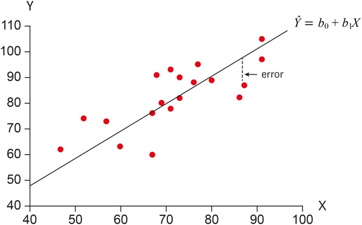
Figure 1A depicts a bivariate relationship with Y, which might represent health problem score, and X, pollution level. As we found in the Correlation section, the scattered points of X and Y pairs show positive relationships which represent a tendency that as X values move positively from their mean, the corresponding Y values also move positively from their own mean, and vice versa. We can try to draw a straight line as close as possible to those data points. However, we cannot connect data points as an exact straight line because generally they do not have a mathematical relationship. The mathematical relationship is expressed by a straight line and the values on the line correspond to values of b₀ + b₁X for various X values as in Figure 1A. We call b₁ and b₀ as slope and intercept, respectively.

Figure 1.

(A) Description of relationship of 2 variables, X and Y; (B) A conceptual relationship between the regression line and surrounding subgroups in the regression model.

Why do we try to express the scattered data points as a straight line? The main idea is that the line represents means of Y for subgroups of X, not individual data points (Figure 1B). Subgroups of X have certain distributions around their means, e.g., normal distribution. Therefore, individual data points can have some distances from the straight line by various amounts of deviations from their means. We call this model as a ‘regression model’ and especially a ‘simple linear regression model’ when only one X variable is included. In the regression model the values on the line is considered as the mean of Y corresponding to each X value and we call the Y values on the line as Ŷ (Y hat), the predicted Y values.

The regression model has been developed as a typical statistical model based on the idea by Francis Galton in 1886 [2]. To establish the simplest typical regression model, we set following four assumptions for the regression model with the acronym ‘LINE’.

• Linear: The means of X subgroups are on the straight line representing the linear relationship between X and Y. In Figure 1b, points on the line represent subgroup means and they are connected as a straight line.

• Independent: The observations are independent to each other, which is a common assumption for general classical statistical models.

• Normal: The X subgroups have normal distribution. Based on this assumption, we could express the full nature of a subgroup only using the mean and variance without any further explanation.

• Equal variance: All the subgroup variances are equal. Based on this assumption, we can simplify the calculation procedure as obtaining a common variance estimate instead of calculating each subgroup variance separately.

Figure 1B depicts the concepts of linear regression by showing the subgroup means (dots) on the straight line and normal distribution of subgroups with equal variances. The scattered dots in Figure 1A are observed points from the subgroup distribution.

LEAST SQUARES METHOD

Above, we tried to draw a straight line as ‘close’ as possible to the data points. In other words, the difference between the line and data points should be minimized. To accomplish the concept mathematically we use the ‘least squares method’. As depicted in Figure 2, the vertical difference between the line and the corresponding data point represents a deviation from the estimated mean (on the line) and actually observed Y value for a specific X value. The deviation is called an ‘error’. The theoretical distribution of errors is assumed as normal distribution as in Figure 1B. The mean of errors in a subgroup is zero and the variance of subgroups is set to a value, e.g., σ².

Figure 2.

Error represents the vertical distance between the line and data point.

The errors are squared and summed to make a squared sum of errors. The least square method aims to minimize the squared sum of errors and to obtain the slope and intercept values which suffice the purpose. The estimated line should show best fit which lies closest to the observed data points. Specifically, we use the first derivatives of squared sum of errors and set the value into zero to get the slope and intercept which produce minimum values of sum of squared errors.

The least square estimates for slope b₁ and intercept b₀ are represented as follows [3]:

$$b_1=\frac{\sum (x-\stackrel{-}{x})(y-\stackrel{-}{y})}{\sum {(x-\stackrel{-}{x})}^2}$$

$$b_0=\stackrel{-}{y}-b_1\stackrel{-}{x}$$

Table 1 displays the calculation procedure using EXCEL. Deviations from means of X and Y (X − X̄ and Y − Ȳ), squares of deviations of X [(X − X̄)²] and cross products of deviations of X and Y [(X − X̄)(Y − Ȳ)] are calculated. Finally, sum of squares of deviations of X and cross products of deviations of X and Y were calculated as 2,912.95 and 2,072.85, respectively. The straight line with least sum of squared errors is obtained finally as: Ŷ = 30.79 + 0.71X.

Table 1. Calculation of least squares estimators of slope and intercept in simple linear regression.

No	X	Y	X−X̿	Y−Y̿	(X−X̄)2	(X−X̄)(Y−Ȳ)
1	73	90	0.55	7.65	0.30	4.21
2	52	74	−20.45	−8.35	418.20	170.76
3	68	91	−4.45	8.65	19.80	−38.49
4	47	62	−25.45	−20.35	647.70	517.91
5	60	63	−12.45	−19.35	155.00	240.91
6	71	78	−1.45	−4.35	2.10	6.31
7	67	60	−5.45	−22.35	29.70	121.81
8	80	89	7.55	6.65	57.00	50.21
9	86	82	13.55	−0.35	183.60	−4.74
10	91	105	18.55	22.65	344.10	420.16
11	67	76	−5.45	−6.35	29.70	34.61
12	73	82	0.55	−0.35	0.30	−0.19
13	71	93	−1.45	10.65	2.10	−15.44
14	57	73	−15.45	−9.35	238.70	144.46
15	86	82	13.55	−0.35	183.60	−4.74
16	76	88	3.55	5.65	12.60	20.06
17	91	97	18.55	14.65	344.10	271.76
18	69	80	−3.45	−2.35	11.90	8.11
19	87	87	14.55	4.65	211.70	67.66
20	77	95	4.55	12.65	20.70	57.56
	X̄ = 72.45	Ȳ = 82.35			∑ = 2,912.95	∑ = 2,072.85

$${\mathit{b}}_1=\frac{\sum (\mathit{x}-\stackrel{-}{\mathit{x}})(\mathit{y}-\stackrel{-}{\mathit{y}})}{\sum {(\mathit{x}-\stackrel{-}{\mathit{x}})}^2}=\frac{2072.85}{2912.95}=0.7116$$

$${\mathit{b}}_0=\stackrel{-}{\mathit{y}}-{\mathit{b}}_1\stackrel{-}{\mathit{x}}=82.35-0.7116*72.45=30.79$$

Using the straight line, we can predict the mean (or predicted) values of Y corresponding to specific X values. Let's discuss an observed data point (73, 90). The predicted value of Y, Ŷ is calculated as 30.79 + 0.7116*73 ≅ 82.74. The error, the deviation between the observed Y and predicted Y value, is around 7.26 (= 90 − 82.74). Like this example, we can apply the estimated regression line in predicting expected Y values and related errors. After establishing estimated regression equation, we need to evaluate it in the aspect of basic assumption and its predicting ability.

Recalling the Pearson correlation coefficient [1], r was calculated as follows:

$$r=\frac{Cov(x,y)}{\mathrm{S}\mathrm{D}\left(X\right)\mathrm{ }\times \mathrm{ }\mathrm{S}\mathrm{D}\left(Y\right)}=\frac{\frac{\sum (x-\stackrel{-}{x})(y-\stackrel{-}{y})}{n-1}}{\mathrm{S}\mathrm{D}\left(X\right)\mathrm{ }\times \mathrm{ }\mathrm{S}\mathrm{D}\left(Y\right)}=\frac{109.1}{12.38\times 12.01}=0.73.$$

The slope can be expressed by r following some procedure such as:

$$b_1=\frac{\sum (x-\stackrel{-}{x})(y-\stackrel{-}{y})}{\sum {(x-\stackrel{-}{x})}^2}=\frac{\frac{\sum (x-\stackrel{-}{x})(y-\stackrel{-}{y})}{n-1}}{\frac{\sum {(x-\stackrel{-}{x})}^2}{n-1}}=\frac{\frac{\sum (x-\stackrel{-}{x})(y-\stackrel{-}{y})}{n-1}}{{\left[SD\right(X\left)\right]}^2}=r\times \frac{SD\left(Y\right)}{SD\left(X\right)}=0.73\times \frac{12.01}{12.38}\cong 0.71.$$

We can use this relationship to calculate slope estimate as well.

Appendix 1

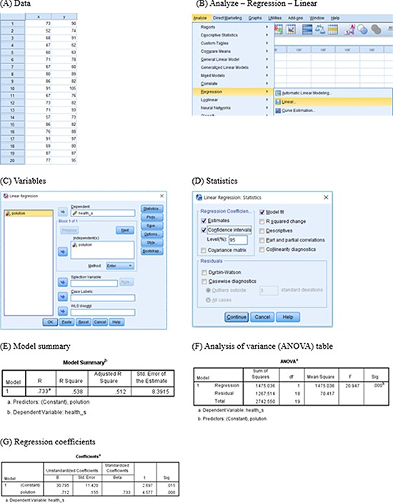
Procedure of analysis of simple linear regression model using IBM SPSS

The procedure of logistic regression using IBM SPSS Statistics for Windows Version 23.0 (IBM Corp., Armonk, NY, USA) is as follows.

References

- 1.Kim HY. Statistical notes for clinical researchers: covariance and correlation. Restor Dent Endod. 2018;43:e4. doi: 10.5395/rde.2018.43.e4. [DOI] [PMC free article] [PubMed] [Google Scholar]
- 2.Galton F. Regression towards mediocrity in hereditary stature. J Anthropol Inst G B Irel. 1886;15:246–263. [Google Scholar]
- 3.Daniel WW. Biostatistics: basic concepts and methodology for health science. 9th ed. New York (NY): John Wiley & Sons; 2010. pp. 410–440. [Google Scholar]