

Abstract
Displaying a single representative conformation of a biopolymer rather than an ensemble of states mistakenly conveys a static nature rather than the actual dynamic personality of biopolymers. However, there are few apparent options due to the fixed nature of print media. Here we suggest a standardized methodology for visually indicating the distribution width, standard deviation and uncertainty of ensembles of states with little loss of the visual simplicity of displaying a single representative conformation. Of particular note is that the visualization method employed clearly distinguishes between isotropic and anisotropic motion of polymer subunits. We also apply this method to ligand binding, suggesting a way to indicate the expected error in many high throughput docking programs when visualizing the structural spread of the output. We provide several examples in the context of nucleic acids and proteins with particular insights gained via this method. Such examples include investigating a therapeutic polymer of FdUMP (5-fluoro-2-deoxyuridine-5-O-monophosphate) – a topoisomerase-1 (Top1), apoptosis-inducing poison – and nucleotide-binding proteins responsible for ATP hydrolysis from Bacillus subtilis. We also discuss how these methods can be extended to any macromolecular data set with an underlying distribution, including experimental data such as NMR structures.
1. Introduction
Discussing the static images of proteins found in journals, Henzler-Wildman and Kern comment, “Physicists, however, will object to a static picture: they see proteins as soft materials that sample a large ensemble of conformations. …” [1] Indeed, we do object. Since the crystallography work by Austin et al. in 1975 on myoglobin [2–4] there is widespread understanding that proteins exist in statistical ensembles of states rather than static conformers, with similar understandings emerging for biopolymers in general [1,4–7]. The specific objection presented here is that despite decades of such knowledge, one of the most basic practices when dealing with distributions of data has yet to become standard for visualizing macromolecules – error bars. Displaying single structures without some indication as to the variance in the distribution those structures represent at best leaves it to the reader to imagine an ensemble and at worst deceives a reader into believing that there is a single state in which the molecule exists [1]. Here we argue for the need to indicate underlying distributions of states when showing macromolecular structures and present statistically rigorous methodologies – involving expected error and standard deviation (see Section 4) – for doing so.
Admittedly, the leap from error bars around a point on a scatter plot or a bar on a histogram to visualizing the uncertainty in a conformation is not obviously straightforward. Therefore, we present several examples and the underlying methodologies. Our first example is of representative structures from Molecular Dynamics (MD) simulations, a useful and increasingly common tool in drug discovery [8,9], generating ever larger ensembles of states as available computational power increases [10,11]. Here we show structures from all-atom MD simulations of a therapeutic oligomer of FdUMP (5-fluoro-2-deoxyuridine-5-O-monophosphate) [12–15]. The large number of structures generated in MD trajectories often requires partitioning conformation space into a handful of macrostates. Typically a representative from each macrostate – say a mean or median structure – is then displayed. However, displaying only the representative with no indication of uncertainty obscures the width of the underlying distribution. We propose a method based on combining clustering – quality threshold clustering [16] for the purposes of this manuscript – combined with statistical analysis as described in Section 4.
As an example of this method’s application to structure prediction and protein-protein interaction (PPI), we show predicted interactions between SufC and SufD, Fig. 4, from Bacillus subtilis [17–24] responsible for ATP hydrolysis and thought to be analogous to similar proteins in Escherichia coli [25]. In addition to the most likely complex, we use the expected error of the PPI calculations to choose additional structures to display – Fig. 4b–d. Our next two examples, Figs. 5 and 6, extend to high-throughput, small ligand docking software that predicts in vivo interactions. Such docking software carries with it an expected error, which we translate to conformation space (see Section 4) and display along with the highest ranked docking pose – Figs. 5b–d and 6b–d. We also discuss how these methods can be extended to any macromolecular data set with an underlying distribution, including experimental data from NMR and X-ray crystallography studies, concluding with a final example of such an application, Fig. 7. To aide others in using these methods, we have made example Python [26] scripts publicly available online [27], supporting information Fig. 1.
Fig. 4.
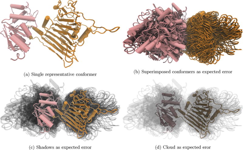
There is a wide variety of relative structure positions in the top 50 docking poses predicted by ZDOCK for SufC (pink) and SufD (orange). We see that SufC’s predicted poses have a wide variety of rotations relative to the top ranked prediction. Representative structures are ZDOCK’s top prediction, and additional frames (b–d) are within the expected error of the top-ranked prediction. (For interpretation of the references to color in this figure legend, the reader is referred to the web version of this article.)
Fig. 5.
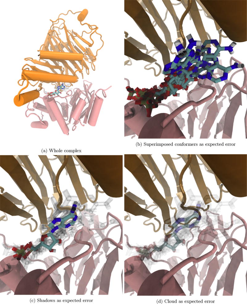
Visualizing the expected error of our docking software indicates high confidence in (a) the general region of the binding site and (b–d) the specific position of the phosphate groups. (For interpretation of the references to color in text near the reference citation, the reader is referred to the web version of this article.)
Fig. 6.
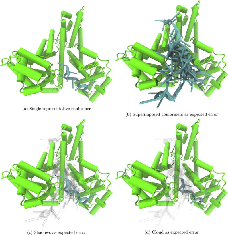
From the localization of F10 docking poses (blue) to one region of albumin (green) within AutoDock Vina’s expected error, we can be more confident in the predicted region of binding F10 than in the conformation that is likely to bind, which has a large variance within the expected error. Representative F10 conformations are Vina’s top prediction, and additional conformers are those within Vina’s expected error of the top prediction. (For interpretation of the references to color in this figure legend, the reader is referred to the web version of this article.)
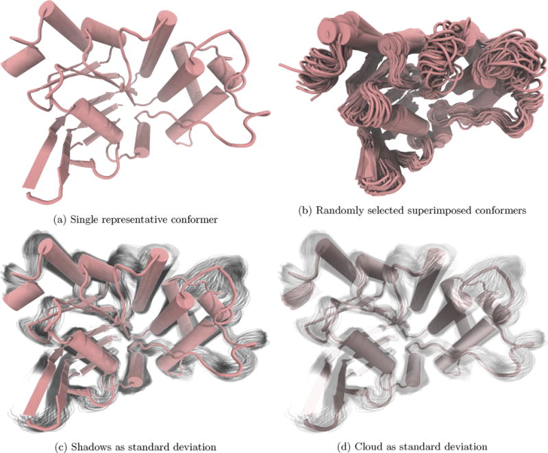
Fig. 7.
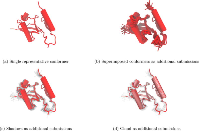
Visualizing multiple conformers of PDB ID 2MRE [56] in addition to the top submission shows that the alpha helix at the right of each panel has a higher relative certainty in its position than the other secondary structure elements.
One common way to show the distribution of states underlying a representative structure is to visualize a superposition of states [28] that have been aligned by minimizing a distance metric between the structures – a method that has been applied to MD, NMR and X-ray crystallography data sets, of which we cite a few examples [28–32]. Within these examples we see both sets of all solid structures superimposed, similar to panel b in all figures herein, where every structure is given equal visual weight. However, this visualization method is often used without a statistically rigorous method for selecting frames. To emphasize the difference between such selection methods and ours, in Figs. 1–3, we choose the additional frames in panel b randomly. In the remaining figures of the paper, we use the statistical measures described in Section 4.
Fig. 1.
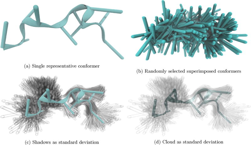
Side-by-side comparison of conformations of F10 in 150 mM CaCl with these four visualization techniques reveals (compare a and b) the deceptiveness of using only a single conformer, (c) the width of the distribution indicated with little loss of visual simplicity, and (d) the ability to see standard deviation in three dimensions.
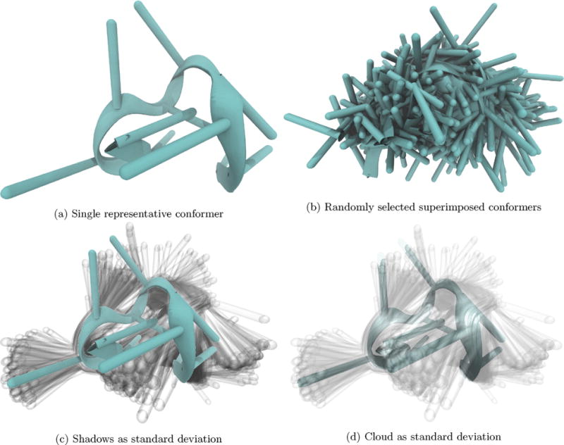
Fig. 3.
In this MD-refined homology prediction of the SufC protein from Bacillus subtilis, we observe little uncertainty in the structured regions relative to the unstructured regions. Representative structures are median, and additional frames randomly selected (b) or one standard deviation (c and d). (For interpretation of the references to color in text near the reference citation, the reader is referred to the web version of this article.)
For displaying additional conformers, we also see the use of transparency, in which a single representative structure is given the most visual weight with the additional conformations seen as a shadow, panel c in all figures, or diffuse cloud, panel d in all figures. For each example system, we include a side-by-side comparison of a traditional structural ensemble diagrams (panels a and b, except Fig. 5) and our suggested styles (panels c and d), drawn with the same representation and viewpoint so that readers may judge for themselves both the value in displaying a clearly defined metric of uncertainty and the usefulness of our preferred visualization styles. No matter the display method, we clearly indicate the statistical metric for choosing these conformations, as the primary point of this work is to show the value in indicating uncertainty in visualization of macromolecule conformers.
Another method is to adjust the width of a residue – or other substituents – based on the width of its distribution of positions [28,33]. These visualizations have the advantage of maintaining the visual simplicity of a single structure and provide information on each substituent’s degree of contribution to overall structural uncertainty. There are also more abstract methods for visualizing these structural varieties, such as that used by Best and Hege to plot sets of interchanging structures or even entire trajectories on planar maps [34]. Such a method brings with it the analysis methods for planar graphs in general [35–38], allowing for a great deal of information to be extracted from the transitions among conformations [34,39,40]. While far less abstract than mapping to a planar graph, the methodology we suggest has a higher level of statistical rigor than simple overlays and is intuitively more straightforward than more abstract methods.
In addition to a representative structure, we choose which substituents to display based on a statistical measure relevant to the data. We display a median – or otherwise representative – structure as solid and each frame in some subset of the distribution as a shadow or cloud – e.g., those falling within one standard deviation of the median, panels c and d in Figs. 1–3, or those within some expected error of the representative, Figs. 4–6. In the shadow representation, overlapping shadows add their opacity to one another, distinguishing between isotropic and anisotropic motion based on the relative darkness of areas in the shadow. In the cloud representations, this distinction is diminished in favor of seeing the variance in three dimensions. Our methods differ from others primarily in the use of a statistical measure – other than random selection, even sampling or the entire distribution width – to choose the superimposed frames. To demonstrate the value of indicating the statistical measure used, we select additional frames using an uncertainty-based cutoff and state the measure used.
2. Results and discussion
2.1. F10 and SufC – MD examples
Applying our visualization method to MD trajectories of a therapeutic oligomer of FdUMP (5-fluoro-2-deoxyuridine-5-O-monophosphate) [12–15], we have observed shifts in the ensemble of preferred structures resulting from the presence of various ions. When visualizing the macrostate representatives (median structure), we include all frames in that macrostate that are within one RMSD-based standard deviation (see Section 4) of the representative conformation. We discern from these visualizations that in the presence of calcium ions, F10 is in a stable but seemingly unstructured state, Fig. 1. We conclude the conformation is unstructured in that it is fully extended and has no obvious base interactions. The small variance in the shadows and cloud, Fig. 1c and d, serves as a conformation space error bar showing one standard deviation.
Comparing this structural ensemble to one from a simulation of F10 in the presence of zinc, Fig. 2, we see that the zinc-solvated distribution of states is more structured but less stable. Additionally, here we see that layering shadows, Fig. 2c, quickly distinguishes between isotropic and anisotropic motion. Bases’ whose motion is more localized show darker in the preferred position, while bases’ whose motion is isotropic have roughly the same opacity over the range of positions. From these variations in shading, we might infer that zinc is preferentially stabilizing some of the bases.
Fig. 2.
By observing the fluctuations about a median structure, we see (in comparison with Fig. 1) that F10 is less structured – i.e., the extent of polymer folding – and more stable in the presence of calcium (seen in Fig. 1) relative to zinc (seen here). Representative structures are median, and additional frames are randomly selected (b) or one standard deviation (c and d) (see Section 4).
Additional analysis needs to be done before formally reporting conclusions about the structure and dynamics of F10 in the presence of various ions. However, we were able to draw immediate, statistics-based inferences about F10 from these visually simple images, panels c and d of Figs. 1 and 2. These examples illustrate the ease and simplicity with which statistically relevant information about biopolymer structural ensembles can be displayed by calculating a standard deviation from some – in this case median – structure and displaying as a shadow or cloud all frames within the distance. While the uncertainty displayed in these images is RMSD-based, the essential idea could be transferred to any measure that can be mapped to conformation space. As demonstrated by analysis of these images, they are able to convey more useful information than the primitive superposition shown in panel b. Furthermore, regardless of the visualization method, the use of a common statistical measure to select the frames in Figs. 1 and 2 allows a reader to immediately understand the information conveyed by the visualization.
Using this visualization method, we have also observed the stability of a homology-predicted structure of SufC from B. subtilis. The lowest order RMSD-based cluster, Fig. 3, captures 50% of the MD frames and shows little variance from the representative structure. Furthermore, the bulk of the fluctuations within that cluster occur in loops. From the conformations within one standard deviation of the median, we see that the alpha helices and beta sheets move little within the cluster relative to the unstructured loop (Fig. 3c and d). Just as in the above nucleic acid example, adding frames within one standard deviation indicates the confidence level in the visualized structure. In this protein example, we see little uncertainty in the secondary structure regions of the protein and more uncertainty in the unstructured regions.
2.2. B. subtilis – a PPI example
In order to suggest candidate residues for mutation studies of B. subtilis, we have predicted the interactions of SufC and SufD – two proteins responsible for ATP hydrolysis when in complex with one another. According to the Critical Assessment of PRedicted Interactions (CAPRI) experiment [41], the set of top 50 predictions returned by PPI software ZDOCK [42–44] for a given system has a 51% chance of containing at least one acceptable structure prediction (defined by an RMSD cutoff from an experimental crystal structure [45,42]). Therefore, in addition to the top ranked ZDOCK prediction, we display the next 49 highest ranked predicted structures as additional conformers, Fig. 4b–d.
From this image, we are immediately able to see the high level of variance in the predicted interactions. The SufD (orange) poses are related to one another by a smaller range of orientations than the SufC (pink) poses. From these observations, we conclude that there is much uncertainty in ZDOCK’s prediction of SufC’s orientations relative to SufD. Additionally, there are no areas of shadow as dark as those in Fig. 2c, indicating little commonality among the positions of secondary structural elements in the top 50 docking predictions. Small shifts would result in much overlap, making some regions of the shadow much darker, as seen in Fig. 2c. By visualizing the uncertainty of PPI output we quickly conclude there is a high level of uncertainty and that we need to either rethink our docking strategy or find a structural refinement methodology that can increase our confidence in the structure predicted before proceeding.
Regardless of how the structure prediction work continues, though, the value in reporting the uncertainty is particularly clear in this example. CAPRI trials report that the top structure from ZDOCK has a 12% chance of being an acceptable structure [42]. If only the top prediction were shown, Fig. 4a, it would be 88% likely our displayed result is not an acceptable docking pose. Hence, visualizing that structure alone would be useless to anyone interested in the interactions between the two proteins. By showing the top 50 predictions, it is more likely than not that an acceptable docking pose is contained therein, and we have made it clear through these additional conformations that there is a high level of variance among the potential interaction geometries.
This system is the clearest of our examples for the utility of our particular visualization scheme (panels c and d in all figures). When the additional conformers within the expected error of ZDOCK are displayed as solid superimposed frames, Fig. 4b, it is difficult to see the secondary structure of any conformation or indeed discern any single conformation at all, a difficulty which is reduced by highlighting a representative structure, Fig. 4c and d. From this example, we hope the reader takes away the general importance of visualizing uncertainty in PPI complex predictions and clearly indicating the measure of error used. Just as showing error bars without indicating the measure they represent would be useless for a viewer, showing the variance in a conformation is not very useful without a clear statement of the associated underlying measure of uncertainty.
2.3. Applications to high throughput ligand docking
Beyond determining the structure of SufC and SufD in complex with one another, we are interested in the complex’s interactions with ATP, Fig. 5. In addition to the model with lowest free energy of binding according to Autodock Vina, we also visualize all predictions within Vina’s expected error of 2.85 kcal/mol of the top model [46], Fig. 5b–d. Immediately, we see that there is a preferred binding pocket, as all models within the expected error of the top are in the same region. Upon zooming in on the ATP binding pocket, Fig. 5b–d, we see that the adenine’s position fluctuates more than the phosphate groups. That is, the adenine base is mostly responsible for the variance in the predicted docking poses. From this observation, we might infer there is a residue on SufC (red) in the binding pocket, that is highly attracted to the negatively charged phosphate groups and that adenine itself may not be directly interacting with the protein complex. Aside from possible interpretations, though, this example demonstrates how visualizing the expected error in small ligand docking allows for interpreting the confidence level of the docking software. In this case, we would be more confident in a predicted position of one of ATP’s phosphate groups than that of the nucleic acid.
We also applied this error visualization scheme to high throughput dockings of F10 to human serum albumin, Fig. 6. After an ensemble docking run, we displayed the top predicted model and all models within AutoDock Vina’s expected error, Fig. 6b–d. From this visualization we see that there is a wide variance in the conformations predicted to dock with albumin. There are two clear commonalities among those docking poses, though. First, all models involve surface docking. Second, within the expected error, F10 prefers to dock to one region of albumin over others with one outlier seen near the bottom of panels b–d in Fig. 6. From a quick analysis of this image, we see that we can be more confident in the general area of likely binding than we can be in a prediction of a specific conformation likely to bind.
2.4. Application to experimental methods
As demonstrated by the above examples, translating a measure of distribution width or uncertainty to conformation space can be done for any ensemble of states. This statement holds not only for computationally predicted structures but also for experimentally derived ensembles. NMR studies of biopolymers in solution sample multiple conformations that can – and should – be reported as ensembles of states, as even the rare conformations found in NMR studies may have significant biological rolls [47,31,48–50,30,51–53]. Therefore, not indicating the ensemble nature of an NMR-derived structure risks missing out on structural variations that result in changes in biological function. Similarly for X-ray crystallography, structural variations across differing crystallization conditions can uncover states of biological import [54,55]. Once such ensembles of states are solved, the visualization methods presented here can be applied just as they were to structures predicted by computational methods.
Consider, for example, an NMR structure of ubiquitin bound to a ubiquitin-binding zinc finger from human Rad18, Fig. 7. This structure is part of the DNA damage tolerance pathway. Rizzo et al. calculated 200 conformers for this complex, submitting 20 of them to the RCSB [56]. By displaying all of the submitted structures with the top submission displayed as solid, we see that the relative position of some structural components are more certain than others. One alpha helix on the right of each panel has almost no shadow, indicating high certainty for this secondary structure element. The other two alpha helices have more variance in their position. The beta sheet near the top alpha helix likewise has little uncertainty in its coordinates relative to the other beta sheets. The loop regions show high variance in their coordinates, which is to be expected from such mobile regions, which are often difficult to resolve in experimental methods. By showing the additional conformers beyond the top submission as shadow, we avoid the visual clutter associated with simple superposition while conveying the relative certainty of structural element positions in the submitted coordinates. This example, though, does raise the question of alignment methods. That is, if the structures are aligned based on a particular secondary structure element, that portion of the polymer would show less variance. Here we aligned to all heavy atoms to avoid biasing the representations as much as possible (see Section 4).
3. Conclusions
Regardless of the specific method employed, it is our primary goal that readers will be motivated to visualize biopolymers (and macromolecules in general) as ensembles of states rather than static conformers in their own works. The nature of such polymers to exist in a distribution of conformations is experimentally known and widely accepted. This fact should be made more evident by the images shown in literature. Additionally, in visualizing the dynamic nature of these molecules, there is little added work in utilizing basic statistical methods to choose which structures from the underlying distribution to display along with a representative. It is, therefore, our secondary goal that those who are moved toward visualizing underlying distributions will do so in ways that are statistically rigorous, just as is typically done on scatter and bar plots.
Additionally, such error reporting is of particular import given the present state of structure determination. At the time of this writing, there are roughly five times as many entries in the Uniprot [57] sequence database as there are in the RCSB [58] structure database. While experimental data is obviously preferred and should be used when available, the ability to predict structures while waiting on – or more precisely, hoping for – a solved crystal structure is a valuable tool in drug discovery [59,60]. Given that computational structure prediction is a presently necessary stop gap, a standardized method for reporting the uncertainty in such predictions is crucial.
We find our specific method of visualizing structural uncertainty to be informative without much loss of visual simplicity. The use of shadows clearly differentiates between the representative structure and those chosen as the structural equivalent of error bars. Additionally, adding the opacity of the shadows shows relative weights in the underlying ensemble and differentiates between isotropic and anisotropic motion in those structures from MD – and could be used similarly for any dynamics-based data set. For those who would like replicate our visualization method, we have made the Python scripts used in making figures in this work available for free online [27], supporting information Fig. 1.
4. Methods
For the layered (shadow) and blended (cloud) images (panels c and d in all figures), we separately visualized representative structures and additional conformers in VMD [61], rendered them with Tachyon [62] and combined the resulting graphics into the images shown here using Pillow, a fork of the Python Image Library. For processing structural data and molecular dynamics trajectories in Python [26], we used the MDTraj library [63]. For the purpose of selecting which frames to include in a given shadow, we stored and processed all data and calculations in NumPy arrays [64]. The method for selecting the frames is based on quality threshold clustering combined with statistical analysis as described below.
The additional conformers in Figs. 1–3 are all frames within one modified standard deviation of the median structure of the lowest order RMSD-based cluster – i.e., highest population cluster – as assigned by the Quality Threshold (QT) [16] algorithm in VMD. For reference, consider the usual form of standard deviation:
where xi is the ith measurement in a given experiment, is the average across all measurements, and N is the number of measurements. For Figs. 1–3, we calculated the RMSD of every conformation in the cluster relative to the median structure. In these images, we do not show the average structure, since it is likely nonphysical. Instead, we show the median structure, and we want our shadows to indicate the variation from this median rather than from the average of all structures in the cluster. Therefore, as a substitute for subtracting the average RMSD – i.e., – we first superposed all structures in the cluster onto the median. That is, we minimized the RMSD of each structure in the ensemble relative to the median structure using rigid body rotations and translations as implemented in the command trajectory.superpose() in the MDTraj library. These alignments are based on all heavy atoms.
Therefore, using ri as the RMSD of a structure from the median and N as the number of structures in the cluster, our modified standard deviation is
The key difference from the usual standard deviation is the measurement of distance from a median rather than a mean. To be clear, we are not advocating for the use of this particular statistical measure for choosing structures to display – though, it is our preference – but rather for the use of some statistical measure that is clearly stated with the figure, just as one would do for error bars on a scatter plot. For those who wish to reproduce or modify this method of frame selection, we have made the script used for generating the images in Figs. 1–3 available online [27], supporting information Fig. 1.
Nucleic acid structures in Figs. 1, 2 and 6 are output from MD simulations run under the canonical ensemble (NVT) in ACEMD [11] simulation software. The single protein in Fig. 3 and the protein-ATP complex shown in Fig. 5 is output from an MD simulation run under the isothermal-isobaric ensemble (NPT) in ACEMD. In all simulations, hydrogen mass repartitioning as implemented in ACEMD allowed us to use 4fs time steps in our production runs. Before beginning these production runs, systems underwent 1000 steps of conjugate-gradient minimization. During simulation, systems were held at 300 K using a Langevin thermostat. For VdW and electrostatic forces, we applied a 9 Å cutoff and 7.5 Å switching distance, calculating long-range electrostatics with a smooth particle mesh Ewald (SPME) summation method [65,66] These simulations were run on Titan GPUs in Metrocubo workstations produced by Acellera. For MD simulations, we solvated nucleic acids in 150 mM MgCl2 and proteins in 150 mM NaCl, using explicit TIP3P water [67] for all biopolymers. For a discussion of counter ion choices, see the review by Lipfert et al. [68].
The individual structures of SufC and SufD from B. subtilis shown as pink and orange respectively in Figs. 3 and 4 are homology predictions made with SWISS-MODEL [69–72]. We predicted the interaction of those two structures with the PPI software ZDOCK [42–44], generating the complexes in Fig. 4. After relaxing the SufC–SufD complex for 1 microsecond as described above, we used AutoDock Vina [46] to predict docking poses for ATP binding. We used this same software to predict docking poses for F10 [73–78,12,13,15,14] and human serum albumin [79]. For the purpose of the simple example in Fig. 5, we used only the SufC–SufD structure from the final frame of the MD simulation. In the docking trial, the receptor (SufC–SufD) was held rigid while the ligand (ATP) was treated as flexible.
Supplementary Material
Acknowledgments
The authors thank Dr. William Gmeiner, Dr. Nicholas Kurniawan, Mr. Ryan Godwin and Mr. Jiajie Xiao for their feedback. This work was partially supported by National Institutes of Health grant R01CA129373. Crystallography & Computational Biosciences services were partially supported by the Comprehensive Cancer Center of Wake Forest University National Cancer Institute grant CCSG P30CA012197.
Appendix A. Supplementary data
Supplementary data associated with this article can be found, in the online version, at http://dx.doi.org/10.1016/j.jmgm.2016.05.001.
References
- 1.Henzler-Wildman K, Kern D. Nature. 2007;450:964–972. doi: 10.1038/nature06522. [DOI] [PubMed] [Google Scholar]
- 2.Austin RH, Beeson KW, Eisenstein L, Frauenfelder H, Gunsalus IC. Biochemistry. 1975;14:5355–5373. doi: 10.1021/bi00695a021. [DOI] [PubMed] [Google Scholar]
- 3.Frauenfelder H, Petsko GA, Tsernoglou D. Nature. 1979;280:558–563. doi: 10.1038/280558a0. [DOI] [PubMed] [Google Scholar]
- 4.Frauenfelder H, Sligar S, Wolynes P. Science. 1991;254:1598–1603. doi: 10.1126/science.1749933. [DOI] [PubMed] [Google Scholar]
- 5.Boehr DD, Nussinov R, Wright PE. Nat Chem Biol. 2009;5:954. doi: 10.1038/nchembio.232. [DOI] [PMC free article] [PubMed] [Google Scholar]
- 6.Fukunishi Y. Expert Opin Drug Metab Toxicol. 2010;6:835–849. doi: 10.1517/17425255.2010.486399. [DOI] [PubMed] [Google Scholar]
- 7.Wrabl JO, Gu J, Liu T, Schrank TP, Whitten ST, Hilser VJ. Biophys Chem. 2011;159:129–141. doi: 10.1016/j.bpc.2011.05.020. [DOI] [PMC free article] [PubMed] [Google Scholar]
- 8.Godwin RC, Melvin R, Salsbury FR. Molecular Dynamics Simulations and Computer-aided Drug Discovery. 2015 [Google Scholar]
- 9.Salsbury FR. Curr Opin Pharmacol. 2010;10:738–744. doi: 10.1016/j.coph.2010.09.016. [DOI] [PMC free article] [PubMed] [Google Scholar]
- 10.Godwin R, Gmeiner W, Salsbury FR. J Biomol Struct Dyn. 2015:1–20. doi: 10.1080/07391102.2015.1015168. [DOI] [PMC free article] [PubMed] [Google Scholar]
- 11.Harvey MJ, Giupponi G, Fabritiis GD. J Chem Theory Comput. 2009;5:1632–1639. doi: 10.1021/ct9000685. [DOI] [PubMed] [Google Scholar]
- 12.Liu J, Kolath J, Anderson J, Kolar C, Lawson TA, Talmadge J, Gmeiner WH. Antisense Nucleic Acid Drug Dev. 1999;9:481–486. doi: 10.1089/oli.1.1999.9.481. [DOI] [PubMed] [Google Scholar]
- 13.Liu J, Skradis A, Kolar C, Kolath J, Anderson J, Lawson T, Talmadge J, Gmeiner WH. Nucleosides Nucleotides. 1999;18:1789–1802. doi: 10.1080/07328319908044843. [DOI] [PubMed] [Google Scholar]
- 14.Liu C, Willingham M, Liu J, Gmeiner WH. Int J Oncol. 2002;21:303–308. [PubMed] [Google Scholar]
- 15.Gmeiner WH, Skradis A, Pon RT, Liu J. Nucleosides Nucleotides. 1999;18:1729–1730. doi: 10.1080/07328319908044836. [DOI] [PubMed] [Google Scholar]
- 16.Heyer LJ. Genome Res. 1999;9:1106–1115. doi: 10.1101/gr.9.11.1106. [DOI] [PMC free article] [PubMed] [Google Scholar]
- 17.Selbach BP, Chung AH, Scott AD, George SJ, Cramer SP, Dos Santos PC. Biochemistry. 2014;53:152–160. doi: 10.1021/bi4011978. [DOI] [PMC free article] [PubMed] [Google Scholar]
- 18.Fang Z, Dos Santos PC. MicrobiologyOpen. 2015;4:616–631. doi: 10.1002/mbo3.267. [DOI] [PMC free article] [PubMed] [Google Scholar]
- 19.Black KA, Dos Santos PC. J Bacteriol. 2015;197:1952–1962. doi: 10.1128/JB.02625-14. [DOI] [PMC free article] [PubMed] [Google Scholar]
- 20.Selbach B, Earles E, Dos Santos PC. Biochemistry. 2010;49:8794–8802. doi: 10.1021/bi101358k. [DOI] [PubMed] [Google Scholar]
- 21.Rajakovich LJ, Tomlinson J, Dos Santos PC. J Bacteriol. 2012;194:4933–4940. doi: 10.1128/JB.00842-12. [DOI] [PMC free article] [PubMed] [Google Scholar]
- 22.Parsonage D, Newton GL, Holder RC, Wallace BD, Paige C, Hamilton CJ, Dos Santos PC, Redinbo MR, Reid SD, Claiborne A. Biochemistry. 2010;49:8398–8414. doi: 10.1021/bi100698n. [DOI] [PMC free article] [PubMed] [Google Scholar]
- 23.Fang Z, Roberts AA, Weidman K, Sharma SV, Claiborne A, Hamilton CJ, Dos Santos PC. Biochem J. 2013;454:239–247. doi: 10.1042/BJ20130415. [DOI] [PubMed] [Google Scholar]
- 24.Black KA, Dos Santos PC. Biochim Biophys Acta (BBA) – Mol Cell Res. 2015;1853:1470–1480. doi: 10.1016/j.bbamcr.2014.10.018. [DOI] [PubMed] [Google Scholar]
- 25.Selbach BP, Pradhan PK, Dos Santos PC. Biochemistry. 2013;52:4089–4096. doi: 10.1021/bi4001479. [DOI] [PubMed] [Google Scholar]
- 26.van Rossum G. Python Reference Manual, CWI, Technical Report CS-R 9525. 1995:1–54. [Google Scholar]
- 27.Melvin R, Salsbury F. figshare. 2015 [Google Scholar]
- 28.O’Donoghue SI, Goodsell DS, Frangakis AS, Jossinet F, Laskowski RA, Nilges M, Saibil HR, Schafferhans A, Wade RC, Westhof E, Olson AJ. Nat Methods. 2010;7:S42–S55. doi: 10.1038/nmeth.1427. [DOI] [PMC free article] [PubMed] [Google Scholar]
- 29.Vammi V, Lin TL, Song G. J Biomol NMR. 2014;58:209–225. doi: 10.1007/s10858-014-9818-2. [DOI] [PubMed] [Google Scholar]
- 30.Thomas MP, McInnes C, Fischer PM. J Med Chem. 2006;49:92–104. doi: 10.1021/jm050554i. [DOI] [PubMed] [Google Scholar]
- 31.Damm KL, Carlson Ha. J Am Chem Soc. 2007;129:8225–8235. doi: 10.1021/ja0709728. [DOI] [PubMed] [Google Scholar]
- 32.Elber R, Karplus M. Science (New York, NY) 1987;235:318–321. doi: 10.1126/science.3798113. [DOI] [PubMed] [Google Scholar]
- 33.Scott WRP, Straus SK. Proteins Struct Funct Bioinf. 2015;83:820–826. doi: 10.1002/prot.24776. [DOI] [PubMed] [Google Scholar]
- 34.Best C, Hege HC. Comput Sci Eng. 2002;4:68–75. [Google Scholar]
- 35.Boccaletti S, Latora V, Moreno Y, Chavez M, Hwang D. Phys Rep. 2006;424:175–308. [Google Scholar]
- 36.Caflisch A. Curr Opin Struct Biol. 2006;16:71–78. doi: 10.1016/j.sbi.2006.01.002. [DOI] [PubMed] [Google Scholar]
- 37.West DB. Introduction to Graph Theory. Vol. 2. Prentice Hall; Upper Saddle River: 2001. [Google Scholar]
- 38.Toussaint GT. Pattern Recognit. 1980;12:261–268. [Google Scholar]
- 39.Böde C, Kovács IA, Szalay MS, Palotai R, Korcsmáros T, Csermely P. FEBS Lett. 2007;581:2776–2782. doi: 10.1016/j.febslet.2007.05.021. [DOI] [PubMed] [Google Scholar]
- 40.Rao F, Caflisch A. J Mol Biol. 2004;342:299–306. doi: 10.1016/j.jmb.2004.06.063. [DOI] [PubMed] [Google Scholar]
- 41.Janin J, Henrick K, Moult J, Eyck LT, Sternberg MJE, Vajda S, Vakser I, Wodak SJ. Proteins Struct Funct Genet. 2003;52:2–9. doi: 10.1002/prot.10381. [DOI] [PubMed] [Google Scholar]
- 42.Pierce BG, Wiehe K, Hwang H, Kim BH, Vreven T, Weng Z. Bioinformatics. 2014;30:1771–1773. doi: 10.1093/bioinformatics/btu097. [DOI] [PMC free article] [PubMed] [Google Scholar]
- 43.Pierce BG, Hourai Y, Weng Z. PLoS ONE. 2011;6:e24657. doi: 10.1371/journal.pone.0024657. [DOI] [PMC free article] [PubMed] [Google Scholar]
- 44.Chen R, Li L, Weng Z. Proteins Struct Funct Genet. 2003;52:80–87. doi: 10.1002/prot.10389. [DOI] [PubMed] [Google Scholar]
- 45.Hwang H, Vreven T, Pierce BG, Hung JH, Weng Z. Proteins Struct Funct Bioinf. 2010;78:3104–3110. doi: 10.1002/prot.22764. [DOI] [PMC free article] [PubMed] [Google Scholar]
- 46.Trott O, Olson AJ. J Comput Chem. 2009;31 doi: 10.1002/jcc.21334. [DOI] [PMC free article] [PubMed] [Google Scholar]
- 47.Philippopoulos M, Lim C. Proteins. 1999;36:87–110. doi: 10.1002/(sici)1097-0134(19990701)36:1<87::aid-prot8>3.0.co;2-r. [DOI] [PubMed] [Google Scholar]
- 48.Huang SY, Zou X. Proteins Struct Funct Bioinf. 2006;66:399–421. [Google Scholar]
- 49.Barril X, Morley SD. J Med Chem. 2005;48:4432–4443. doi: 10.1021/jm048972v. [DOI] [PubMed] [Google Scholar]
- 50.Sheridan RP, McGaughey GB, Cornell WD. J Comput Aided Mol Des. 2008;22:257–265. doi: 10.1007/s10822-008-9168-9. [DOI] [PubMed] [Google Scholar]
- 51.Korzhnev DM, Kay LE. Acc Chem Res. 2008;41:442–451. doi: 10.1021/ar700189y. [DOI] [PubMed] [Google Scholar]
- 52.Yu D, Volkov AN, Tang C. J Am Chem Soc. 2009;131:17291–17297. doi: 10.1021/ja906673c. [DOI] [PubMed] [Google Scholar]
- 53.Berlin K, Castañeda CA, Schneidman-Duhovny D, Sali A, Nava-Tudela A, Fushman D. J Am Chem Soc. 2013;135:16595–16609. doi: 10.1021/ja4083717. [DOI] [PMC free article] [PubMed] [Google Scholar]
- 54.Kohn JE, Afonine PV, Ruscio JZ, Adams PD, Head-Gordon T. PLoS Comput Biol. 2010;6:e1000911. doi: 10.1371/journal.pcbi.1000911. [DOI] [PMC free article] [PubMed] [Google Scholar]
- 55.Fraser JS, van den Bedem H, Samelson AJ, Lang PT, Holton JM, Echols N, Alber T. Proc Natl Acad Sci. 2011;108:16247–16252. doi: 10.1073/pnas.1111325108. [DOI] [PMC free article] [PubMed] [Google Scholar]
- 56.Rizzo AA, Salerno PE, Bezsonova I, Korzhnev DM. Biochemistry. 2014;53:5895–5906. doi: 10.1021/bi500823h. [DOI] [PubMed] [Google Scholar]
- 57.Consortium TU. Nucleic Acids Res. 2015;43:D204–D212. doi: 10.1093/nar/gku989. [DOI] [PMC free article] [PubMed] [Google Scholar]
- 58.Berman HM. Nucleic Acids Res. 2000;28:235–242. doi: 10.1093/nar/28.1.235. [DOI] [PMC free article] [PubMed] [Google Scholar]
- 59.Congreve M, Murray CW, Blundell TL. Drug Discov Today. 2005;10:895–907. doi: 10.1016/S1359-6446(05)03484-7. [DOI] [PubMed] [Google Scholar]
- 60.Cheng T, Li Q, Zhou Z, Wang Y, Bryant SH. AAPS J. 2012;14:133–141. doi: 10.1208/s12248-012-9322-0. [DOI] [PMC free article] [PubMed] [Google Scholar]
- 61.Humphrey W, Dalke A, Schulten K. J Mol Graph. 1996;14:33–38. doi: 10.1016/0263-7855(96)00018-5. [DOI] [PubMed] [Google Scholar]
- 62.Stone J. Ph D thesis. Computer Science Department, University of Missouri-Rolla; 1998. An Efficient Library for Parallel Ray Tracing and Animation. [Google Scholar]
- 63.McGibbon RT, Beauchamp KA, Harrigan MP, Klein C, Swails JM, Hernández CX, Schwantes CR, Wang LP, Lane TJ, Pande VS. Biophys J. 2015;109:1528–1532. doi: 10.1016/j.bpj.2015.08.015. [DOI] [PMC free article] [PubMed] [Google Scholar]
- 64.van der Walt S, Colbert SC, Varoquaux G. Comput Sci Eng. 2011;13:22–30. [Google Scholar]
- 65.Darden T, York D, Pedersen L. J Chem Phys. 1993;98:10089. [Google Scholar]
- 66.Harvey MJ, De Fabritiis G. J Chem Theory Comput. 2009;5:2371–2377. doi: 10.1021/ct900275y. [DOI] [PubMed] [Google Scholar]
- 67.Jorgensen WL, Chandrasekhar J, Madura JD, Impey RW, Klein ML. J Chem Phys. 1983;79:926. [Google Scholar]
- 68.Lipfert J, Doniach S, Das R, Herschlag D. Annu Rev Biochem. 2014;83:813–841. doi: 10.1146/annurev-biochem-060409-092720. [DOI] [PMC free article] [PubMed] [Google Scholar]
- 69.Biasini M, Bienert S, Waterhouse A, Arnold K, Studer G, Schmidt T, Kiefer F, Cassarino TG, Bertoni M, Bordoli L, Schwede T. Nucleic Acids Res. 2014;42:W252–W258. doi: 10.1093/nar/gku340. [DOI] [PMC free article] [PubMed] [Google Scholar]
- 70.Arnold K, Bordoli L, Kopp J, Schwede T. Bioinformatics. 2006;22:195–201. doi: 10.1093/bioinformatics/bti770. [DOI] [PubMed] [Google Scholar]
- 71.Kiefer F, Arnold K, Kunzli M, Bordoli L, Schwede T. Nucleic Acids Res. 2009;37:D387–D392. doi: 10.1093/nar/gkn750. [DOI] [PMC free article] [PubMed] [Google Scholar]
- 72.Guex N, Peitsch MC, Schwede T. Electrophoresis. 2009;30:S162–S173. doi: 10.1002/elps.200900140. [DOI] [PubMed] [Google Scholar]
- 73.Gmeiner WH, Lema-Tome C, Gibo D, Jennings-Gee J, Milligan C, Debinski W. J Neurooncol. 2014;116:447–454. doi: 10.1007/s11060-013-1321-1. [DOI] [PMC free article] [PubMed] [Google Scholar]
- 74.Pardee TS, Stadelman K, Jennings-Gee J, Caudell DL, Gmeiner WH. Onco-target. 2014;5:4170–4179. doi: 10.18632/oncotarget.1937. [DOI] [PMC free article] [PubMed] [Google Scholar]
- 75.Pardee TS, Gomes E, Jennings-Gee J, Caudell D, Gmeiner WH. Blood. 2012;119:3561–3570. doi: 10.1182/blood-2011-06-362442. [DOI] [PMC free article] [PubMed] [Google Scholar]
- 76.Gmeiner WH, Reinhold WC, Pommier Y. Mol Cancer Ther. 2010;9:3105–3114. doi: 10.1158/1535-7163.MCT-10-0674. [DOI] [PMC free article] [PubMed] [Google Scholar]
- 77.Liao ZY, Sordet O, Zhang HL, Kohlhagen G, Antony S, Gmeiner WH, Pommier Y. Cancer Res. 2005;65:4844–4851. doi: 10.1158/0008-5472.CAN-04-1302. [DOI] [PubMed] [Google Scholar]
- 78.Bijnsdorp IV, Comijn EM, Padron JM, Gmeiner WH, Peters GJ. Oncol Rep. 2007;18:287–291. doi: 10.3892/or.18.1.287. [DOI] [PubMed] [Google Scholar]
- 79.Bhattacharya AA, Grüne T, Curry S. J Mol Biol. 2000;303:721–732. doi: 10.1006/jmbi.2000.4158. [DOI] [PubMed] [Google Scholar]
Associated Data
This section collects any data citations, data availability statements, or supplementary materials included in this article.