Hierarchical Vertex Regression-Based Segmentation of Head and Neck CT Images for Radiotherapy Planning

Abstract

Segmenting organs at risk from head and neck CT images is a prerequisite for the treatment of head and neck cancer using intensity modulated radiotherapy. However, accurate and automatic segmentation of organs at risk is a challenging task due to the low contrast of soft tissue and image artifact in CT images. Shape priors have been proved effective in addressing this challenging task. However, conventional methods incorporating shape priors often suffer from sensitivity to shape initialization and also shape variations across individuals. In this paper, we propose a novel approach to incorporate shape priors into a hierarchical learning-based model. The contributions of our proposed approach are as follows: 1) a novel mechanism for critical vertices identification is proposed to identify vertices with distinctive appearances and strong consistency across different subjects; 2) a new strategy of hierarchical vertex regression is also used to gradually locate more vertices with the guidance of previously located vertices; and 3) an innovative framework of joint shape and appearance learning is further developed to capture salient shape and appearance features simultaneously. Using these innovative strategies, our proposed approach can essentially overcome drawbacks of the conventional shape-based segmentation methods. Experimental results show that our approach can achieve much better results than state-of-the-art methods.

I. Introduction

Head and neck cancer (H&NC) is the fifth most common cancer diagnosed worldwide and the eighth most common cause of cancer death [1]. Intensity modulated radiotherapy (IMRT) can deliver precise radiation doses to a tumor while minimizing the dose to organs at risk (OARs). Therefore, IMRT has become the state of the art method for the treatment of H&NC. When treating H&NC using IMRT, the accurate delineation of OARs from H&N CT images is an essential step. However, it is a tedious and time-consuming task to delineate OARs manually. Moreover, the intra- and inter-rater variability by manual delineation [2]–[4] can directly influence the treatment performance of IMRT. Consequently, it is clinically desirable to develop computer-aided methods to automatically and accurately segment OARs from H&N CT images.

However, it is difficult to accurately and automatically segment OARs from CT images due to low contrast of soft tissue and image artifact (e.g., caused by dental implants) in CT images, as well as the variations of OARs across individuals. Many methods have been proposed to address these challenges. For example, Street et al. [5] developed a 3D level set based computerized system for automatically segmenting a diverse set of lesions in H&N CT scans. On the other hand, since atlases can provide prior information, atlas-based segmentation method is also a hot topic for researchers. Han et al. [6] proposed an atlas-based method for automatic segmentation of critical structures and lymph node regions in the given H&N CT images. Both Levendag et al. [7] and Sims et al. [8], respectively, gave a clinical assessment of their atlas-based method in automatically delineating OARs from H&N CT images. In order to obtain the closed surfaces, active contours [9] or graph cuts [10] were further used to postprocess the results of the atlas-based segmentation. In recent years, the deep nets based methods, such as fully convolutional network (FCN) [11], U-Net [12] and Generative Adversarial Nets (GANs) [13], has been proven effective in semantic image segmentation [14], [15] as well as medical image segmentation [16]–[18]. But, to our knowledge, there are no reports of applying deep learning to H&N CT image segmentation so far.

Incorporating shape prior knowledge of the target object into the segmentation problem can often significantly improve the segmentation performance [19]–[28], especially when having blurred boundaries in the target organ. Among all shape prior based segmentation methods, deformable model based segmentation methods can directly incorporate shape priors to regularize the final segmentation of the target organ and have been widely used to segment organs from CT images. For example, statistical appearance models and geodesic active contours were combined with multi-atlases based segmentation to segment OARs from H&N CT images [29]. The methods presented in [30]–[33] also used deformable shape model to segment organs from pelvic CT images.

However, most of the deformable model based segmentation methods have two disadvantages: (1) Sensitivity to initialization. In the process of refining the locations of model points, these methods usually perform simple gradient-descent optimization, and thus can be easily trapped into local minima, with poor segmentation [34]. (2) Insufficient robustness to shape variations of target organ across individuals. In the conventional deformable model based segmentation methods [35]–[37], local search strategy is often used to refine the shape model. Specifically, after the shape model is initialized, each vertex of deformable model locally searches along its normal direction to find its new position with the maximum boundary likelihood, e.g., the maximum intensity gradient magnitude. Nevertheless, due to the shape variations among individuals, the ground-truth location of a model point is likely not exactly in the normal direction, and thus the shape prior at this vertex will provide incorrect constraint to the final segmentation.

In this paper, we propose a novel shape prior based method to automatically segment OARs from H&N CT images for radiotherapy planning. The main idea is based on the fact that some points on the organ boundaries are more distinctive in image appearance and thus can be more critical in describing shapes of the target organs. In the following, we will simply refer to the distinctive and critical points as critical boundary points. The most critical boundary points can be easily detected, which can then be used to help locate other less critical boundary points. By iterating this procedure, more and more boundary critical points can be located hierarchically. Finally, these located critical boundary points can be used to carry out the organ segmentation. Our key idea is to identify and locate critical boundary points hierarchically, especially using the previously located critical points to guide the detection of next less critical boundary points.

In our work, the above idea is achieved by our proposed random forest (RF) based iterative learning framework. Specifically, in the training stage, the learning framework starts with the construction of the organ shape model, which is composed of model vertices sparsely distributed on the organ surface. Then, regression forest is employed to train the iterative vertex regression forests for estimating the locations of model vertices in the new testing image. In the first iteration, for each model vertex in the shape model, we employ a regression forest to train a vertex regression forest that can predict the 3D displacement from a testing image voxel to each model vertex, based only on the surrounding appearance features of this testing image voxel. To identify the most critical vertices, all available atlases are partitioned to the training and validation sets, and the validation set is used to evaluate the performance of vertex regression forests trained using the training set. Then, the vertices that can be accurately predicted are regarded as the most critical model vertices. In the following iterations, the vertex regression forests learned in the previous iteration are first applied to each training image to generate displacement maps over the entire image domain. Then, with both the appearance features from intensity image and the shape prior from the estimated displacement maps, for each model vertex, a second vertex regression forest is trained. By repeating this procedure, more and more critical vertices can be hierarchically located. Once every model vertex is iteratively evaluated and included into the hierarchical set of critical model vertices, we can further employ classification forest to obtain the final segmentation, which can be trained by both the appearance features from intensity images and the shape prior from the displacement maps (that are generated by applying our trained iterative vertex regression forests).

The testing stage is similar to the above training stage. That is, given a testing image, our trained iterative vertex regression model is first used to hierarchically predict the locations of all model vertices in the testing image space, and then our trained classification forest is applied to obtain the final segmentation result.

The main contributions of our work are as follows:

1. We present a novel learning-based mechanism to locate critical model vertices. This mechanism is able to identify critical model vertices with distinctive appearance and strong across-subject consistency.

2. We also propose a hierarchical strategy for vertex regression. Specifically, the most critical model vertices are located first. Then, with the spatial guidance from these most critical model vertices, other less critical model vertices can be gradually located. By iterating this process, all model vertices can be hierarchically located. The use of this strategy makes our segmentation very robust.

3. We further develop a framework to jointly learn shape and appearance. In particular, both the shape information from the spatial configuration of vertices and the appearance information from intensity image are captured simultaneously in the regression forests.

The rest of the paper is organized as follows. Section II introduces our hierarchical vertex regression based segmentation method. Experimental results are presented in Section III. Conclusions are given in Section IV.

II. Method

A. Notations

An atlas library 𝔸 consists of multiple atlases {Aⁿ = (Iⁿ, Lⁿ) |n = 1, 2,⋯, N}, where Iⁿ and Lⁿ are the intensity image and the label image of the n^th atlas, and N is the total number of atlases in the atlas library.

𝔸 is deformed to

$$\left\{A_{\mathit{warp}}^n=\left(I_{\mathit{warp}}^n,L_{\mathit{warp}}^n\right)\mid n=1,2,\cdots ,N\right\}$$

using groupwise registration [38].

In this work, an organ shape is represented by a Point Distribution Model [35]. Let S denote the target organ shape. A set of landmarks sparsely distributed on S construct a vertex set V = {v₁, ⋯, v_m, ⋯, v_M}, where v_m ∈ ℝ³(m = 1, 2, ⋯, M) is the vector of 3D coordinate of the m^th landmark, and M is the total number of landmarks.

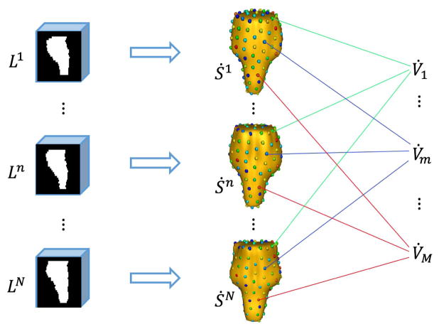
Given N label images in 𝔸, N shape instances Ṡ = {Ṡⁿ|n = 1, 2, ⋯, N} are constructed by shape correspondence method with the corresponding vertex sets 𝕍̇ = {V̇ⁿ|n = 1, 2, ⋯, N}. Here, ${\stackrel{.}{V}}^n=\{{\stackrel{.}{v}}_1^n,\cdots ,{\stackrel{.}{v}}_m^n,\cdots ,{\stackrel{.}{v}}_M^n\}$ are the M landmarks on shape instance Ṡⁿ, and ${\stackrel{.}{v}}_m^n$ is the m^th landmark on the n^th shape instance Ṡⁿ. The m^th landmark on all N shape instances can construct a correspondence vertex set ${\stackrel{.}{V}}_m=\{{\stackrel{.}{v}}_m^1,\cdots ,{\stackrel{.}{v}}_m^n,\cdots ,{\stackrel{.}{v}}_m^N\}$, where all vertices are corresponding to each other. That is, each vertex ${\stackrel{.}{v}}_m^n(n=1,2,\cdots ,N)$ represents the same anatomical location of different shape instances.

In this paper, the target organ shape is modeled by the vertex set V, as well as the spatial relationships between vertices in V, i.e., the relative positions of each vertex to other vertices. Note that our proposed RF based learning framework can learn these spatial relationships from multiple shape instances in 𝕊̇ without the need for explicit formula.

In our method, atlas-based segmentation is formulated as a machine learning problem, where heuristics and prior knowledge are learned from the atlas library 𝔸 and then used to segment a new image I^test. We apply random forest algorithm to address this learning problem. And there are J cascaded multilevel regressions and one classifier in our framework, and the j^th regression is denoted as R_j, j = 1, 2, ⋯, J. For each regression forest R_j, a critical vertex set ℂ_j = {C_m,j |m = 1, 2, ⋯, M_j} is constructed and also a corresponding regression forest set 𝔽_j = {F_m,j |m = 1, 2, ⋯, M_j} is trained, where m is the index of critical vertex and M_j is the total number of critical vertices in ℂ_j. By applying F_j on a deformed testing image $I_{\mathit{warp}}^{\mathit{test}}$, a set of estimated displacement maps ${\widehat{\mathbb{Y}}}_j^{\mathit{test}}=\left\{{\widehat{Y}}_{m,j}^{\mathit{test}}\mid m=1,2,\cdots ,M_j\right\}$ can be generated. For the classification forest F_C, it is trained to complete the segmentation and provide the final segmentation result, i.e., the final label image L_out.

B. Method Overview

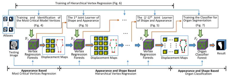
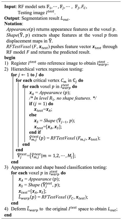
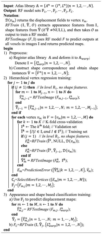
Algorithm I gives a training procedure of our proposed method. Before the training procedure, we perform atlas preprocessing, including atlas registration, shape instances extraction and correspondence construction, which converts the N training label images {Lⁿ|n = 1, 2, ⋯, N} into the N shape instances represented by the corresponding vertex sets 𝕍̇. After preprocessing, our proposed RF based hierarchical vertex regression and target organ classification framework (Fig. 1) utilizes the shape features extracted from 𝕍̇ and the appearance features extracted from intensity images {Iⁿ|n = 1, 2, ⋯, N} to construct regression and classification models, which are applied to a testing intensity image I^test to generate its final segmentation result. Algorithm II gives the testing pipeline of our proposed method.

Fig. 1.

The overview flowchart for our proposed hierarchical vertex regression based organ segmentation. 𝔽₁, 𝔽₂, 𝔽_J and F_C are the 1^st, 2^nd, J^th regression forests and the classification forest, respectively, which are learned in the training procedure.

There are three major steps in our proposed learning framework:

1. Appearance Based Most Critical Vertices Regression: (shown in the left part of Fig. 1)

In this step, we first use the appearance features extracted from the training CT images to train our vertex regression forests. Then, we validate them on the -validation CT images to identify the most critical model vertices with the smallest prediction errors by our trained vertex regression forests. In this way, we can use the vertex regression forests for the most critical vertices (identified) to guide the selection of next less critical vertices in the subsequent step.

2. Appearance and Shape Based Hierarchical Vertex Regression: (shown in the middle part of Fig. 1)

There are several sequentially connected iterative regressors in this step. Each regressor is trained based on both the appearance features from CT images and the shape features from the displacement maps estimated by previous regressors. In each iteration, more new critical model vertices are identified and their corresponding vertex regression forests are learned; meanwhile, the vertex regression forest for the critical model vertices identified in the previous iterations are re-trained with the new shape features for refinement. Note that, in the testing stage, the learned regressors are sequentially applied to the testing CT image to hierarchically locate those critical model vertices.

Algorithm 1.

Training Pipeline of Our Proposed Hierarchical Vertex Regression Based Organ Segmentation

Algorithm 2.

Testing Pipeline of Our Proposed Hierarchical Vertex Regression Based Organ Segmentation

3. Appearance and Shape Based Organ Classification: (shown in the right part of Fig. 1)

In this step, both the appearance features from CT images and the shape prior from displacement maps of critical model vertices are used to train a classifier forest, which is employed to achieve the final segmentation of target organ.

In the rest of this section, we will first describe the preprocessing procedure, then briefly introduce RF and its implementation in our method, and finally give the detailed descriptions of the three main steps aforementioned.

C. Preprocessing

1) Registration

In order to eliminate the orientation difference across atlases {Aⁿ = (Iⁿ, Lⁿ) |n = 1, 2, ⋯, N}, groupwise registration [38] is needed. Accordingly, we first use a groupwise registration toolbox GLIRT (http://www.nitrc.org/projects/glirt) to estimate an unbiased group mean image Ī, which is used as the reference image in this paper. Then, all intensity images are affine registered onto this reference image Ī by the registration toolbox Elastix (http://elastix.isi.uu.nl). Similarly, all corresponding label images of atlases are affine transformed into the reference image space for generating a set of registered atlases ${\mathbb{A}}_{\mathit{warp}}=\left\{A_{\mathit{warp}}^n=\left(I_{\mathit{warp}}^n,L_{\mathit{warp}}^n\right)\mid n=1,2,\cdots ,N\right\}$.

2) Shape Correspondence

Shape correspondence aims at identifying a set of corresponding landmarks across a population of shape instances. Shape correspondence construction algorithms, as well as their evaluations, have been widely investigated in the past years [39], [40]. In this paper, an entropy-based particle systems algorithm [41], [42] is used to construct shape correspondence, although other advanced methods can also be applied.

As shown in Fig. 2, each registered label image $L_{\mathit{warp}}^n(n=1,2,\cdots ,N)$ in the atlas library represents an organ shape instance Ṡⁿ. After shape correspondence detection, we obtain N corresponding vertex sets 𝕍̇ = {V̇ⁿ|n = 1, 2, ⋯, N}.

Fig. 2.

Schematic diagram of constructing 3D shape model and establishing correspondences.

Then the mean shape S̄ is calculated by averaging over the locations of the corresponding vertices across all the 3D shape instances, i.e., S̄ = {v̄_m|m = 1, 2, ⋯, M}, where ${\overline{v}}_m={\sum }_{n=1}^N{v}_m^n/N$. In the following section, S̄ is used to determine the neighborhood relationship of vertices in V.

D. Random Forest Based Regression and Classification

As mentioned in Section II.B, our learning framework is based on RF. In this section, we will give a brief introduction about RF and its implementation in our work.

RF [36], [43]–[50], an efficient model for a variety of learning tasks, has been widely used and shown great performance in image processing. It ensembles a number of trained decision trees to produce an accurate prediction for an unseen data. As a general learning model, the use of RF has two phases: training and testing.

1) Training Phase

The goal of training is to optimize the parameters of split function at each split tree node in RF and to determine the leaf node distributions. For each tree in a RF, a training example set D is randomly sampled, i.e., D = {(x₁, y₁), ⋯, (x_w, y_w), ⋯, (x_W, y_W)}, where x_w ∈ ℱ is an input K-dimensional feature vector and y_w is the output with respect to x_w. The split function at a split node is a function with binary output:

$$f_{l,\mathcal{T}}\triangleq (B·\mathit{x}\ge \mathcal{T})$$ (1)

where B is a K-dimensional binary vector with only one (l^th) non-zero entry and 𝒯 ∈ ℝ is a threshold. The D is simultaneously pushed through all the trees. Let D_p denote the sample set arriving at the split node p, where D₀ = D at the root node. At each split node, D_p is divided into two subsets according to the result of split function and they are sent to the left or right child node separately. The tree grows by iteratively splitting of the training data until it reaches a predefined depth or the sample number at a node is less than a predefined threshold. Each leaf node of the trees stores the empirical distribution of output target y over the incoming subset of training data.

2) Testing Phase

A previously unseen input feature vector x_test is simultaneously pushed through all trees of RF. Starting at the root, each split node applies its associated split function f_l,T to x_test. According to the result of split function, the input data x_test is sent to the left or right child node. This process is repeated until x_test reaches a leaf node. The empirical distribution of output y stored in the respective leaf node provides a prediction for the testing data x_test. All the predictions of all trees in a forest are averaged to gain an overall prediction ŷ for the target value.

If the output y associated with an input data is continuous, the RF is a regression forest and can be used for the nonlinear regression of dependent variables given independent input. If the output y is discrete, the RF is a classification forest and can be used to produce probabilistic output with the likelihood of the input data belonging to a certain class.

In this paper, both regression forest and classification forest are used. Specifically, regression forest is used to predict the 3D displacement vector, pointing from a query voxel in CT image to a model vertex in the shape model. And, classification forest aims to predict the likelihood of a query voxel belonging to a target organ.

It is very important for RF to select suitable features as the input. Due to serious noise in CT images, it is not effective of directly using image intensities as features. Haar-like features, a kind of low-level appearance features extracted from local intensity patches, are robust to noise and can be computed very rapidly using integral image. Also, Haar-like features have shown high performance in many applications [37], [51]–[53].

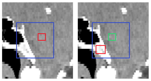
Thus, in this paper, we use the scheme of [53] and consider two types of Haar-like features. The first type is one-block Haar-like features which calculate the average intensity of a block at a location within the local intensity patch. The second type is two-block Haar-like features which compute the average intensity difference between two blocks at two locations within the local intensity patch. The mathematical definition of the Haar-like features used in this paper is formulated as follows:

$$f(I_o\mid c_1,s_1,c_2,s_2)=\frac{1}{{(2s_1+1)}^3}\sum _{\Vert d-c_1\Vert \le s_1}{I}_o(d)-\frac{\lambda }{{(2s_2+1)}^3}\sum _{\Vert d-c_2\Vert \le s_2}{I}_o(d)$$ (2)

where I_o denotes a local intensity patch centered at voxel o and I_o (d) returns the intensity of the image at voxel d. f (I_o|c₁, s₁, c₂, s₂) denotes one Haar-like feature with parameters {c₁, s₁, c₂, s₂}, where c₁ ∈ ℝ³ and s₁ ∈ ℝ are the center and size of the positive block, respectively, and c₂ ∈ ℝ³ and s₂ ∈ R are the center and size of the negative block, respectively. Here, λ ∈ {0, 1} is a switch between the two types of Haar-like features. When λ is 0, Eq. (2) denotes one-block Haar-like features; When λ is 1, Eq. (2) denotes two-block Haar-like features. Fig. 3 gives the graphical illustration of how the Haar-like features are computed.

Fig. 3.

Illustration of calculation of Haar-like features. Left: One-block Haar-like features. Right: Two-block Haar-like features. Blue, red and green rectangles denote the local intensity patch, the positive block, and the negative block, respectively.

It is worth noting that features are calculated over the blocks, instead of the patches, and the block size will not change with the patch size. Therefore, a larger patch size will not result in the blurred features.

In fact, the exhaustive Haar-like feature space is very large and overcomplete, even for a patch size with practical value [52]. In our work, we randomly sample a feature sub-space to resolve this problem. To train a tree in the RF, we adopted two types of random sampling. The first is to generate a Haar-like random feature sub-space _sub by randomly setting λ to 0 or 1 and by uniformly and randomly sampling parameters {c₁, s₁, c₂, s₂}, under the constraint that both positive and negative blocks should stay within the local patch. The second is to randomly sample voxels from each training atlas and then extract feature vector according to the feature sub-space ℱ_sub for constructing the training example set D.

In order to include the discriminative features in ℱ_sub, the number of extracted Haar-like features in ℱ_sub is quite large. Random forest is able to distinguish discriminative features from all extracted Haar-like features during the training, thus it is used as a regression or classifier technique in our proposed method.

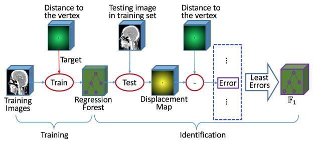
E. Training and Identification of the Most Critical Model Vertices

Since all the vertices in a correspondence vertex set V̇_m are at the corresponding positions of all the 3D shapes, their appearance features from intensity image should be consistent with each other to some extent. But, some correspondence vertex sets have stronger distinctiveness in appearance and more consistency across individuals, than other correspondence vertex sets. Thus, these critical vertices are easier to be detected. The main purpose of this subsection is to identify the most critical model vertices, as well as to learn the respective regression forests to detect them. The flowchart for these tasks is shown in Fig. 4.

Fig. 4.

Flowchart for training and identification of the most critical model vertices.

1) Appearance Based Vertex Regression

For each correspondence vertex set V̇_m, we train a regression forest F_m. To train a tree in F_m, we first construct training example data set D. As mentioned in Section II.D, the Haar-like feature sub-space ℱ_sub is first constructed by randomly sampling from the whole Haar-like feature space. Then, we randomly sample a number of voxels from each atlas and extract a feature vector from a CT image for every sampled voxel to generate a training input data X = {x₁, ⋯, x_w, ⋯, x_W}, where W is the total number of voxels sampled from all the atlases. For the w^th sampled voxel p_w, supposing that it is sampled from the n^th atlas, the 3D displacement vector y_w ∈ ℝ³ from the voxel p_w to the ground-truth vertex ${\stackrel{.}{v}}_m^n$ is computed, i.e., ${\mathit{y}}_w=p_w-{\stackrel{.}{v}}_m^n$. With the training example set D ={(x₁, y₁), ⋯, (x_w, y_w), ⋯, (x_W, y_W)}, a tree can be trained by the regular exhaustive search optimization method. After vertex-wisely training, we get totally M regression forests, one forest for one correspondence vertex set.

2) Identification of the Most Critical Model Vertices

Meanwhile, given a new registered validation CT image $I_{\mathit{warp}}^{\mathit{vali}}$, our goal is to estimate the positions of all the vertices of the shape model in $I_{\mathit{warp}}^{\mathit{vali}}$. For a voxel p of the validation CT image $I_{\mathit{warp}}^{\mathit{vali}}$, the Haar-like feature vector x_vali is first extracted from the local intensity patch centered at p. And then the prediction value ${\widehat{\mathit{y}}}_m^{\mathit{vali}}$, i.e., the 3D displacement vector from p to the m^th vertex v_m of the shape model, is estimated by pushing x_vali through all the trained trees in F_m. All voxel-wisely predicted 3D displacement vectors construct a 3D displacement map ${\widehat{Y}}_m^{\mathit{vali}}$, which can be regarded as a vector image with the image size as the same as $I_{\mathit{warp}}^{\mathit{vali}}$.

As previously described, those critical vertices in the shape model have more distinctive appearance in each individual subject and are also more consistent across individual subjects. These properties can be captured by the trained regression forests, i.e., their performances in predicting the locations of model vertices. According to this observation, we propose below a mechanism to identify the most critical model vertices.

Since the ground-truth vertex positions for the training data are known, we can use CT images in the atlas library as validation images (i.e., in a K-fold cross-validation fashion) to inspect the prediction accuracy of the learned regression forests. Specifically, the training atlases are divided into K subgroups. For each vertex v_m in the shape model, atlases in all K − 1 subgroups are used as the training data to train a regression forest F_m, while atlases in the remaining subgroup are used as the validation data to validate the model F_m. This cross-validation process is repeated K times, with each of the K subgroups used exactly once as a validation data. Finally, we obtain N predicted 3D displacement maps $\left\{{\widehat{Y}}_m^n\mid n=1,2,\cdots ,N\right\}$ for each shape model vertex v_m.

Meanwhile, by directly computing the 3D displacement vector from each voxel of $I_{\mathit{warp}}^n$ to the ground-truth location of vertex ${\stackrel{.}{v}}_m^n$, we get the ground-truth 3D displacement field $Y_m^n$. Then, the prediction error to $I_{\mathit{warp}}^n$ can be computed by the following equation:

$$e_m^n=\frac{1}{{\mathit{VOL}}_{\mathrm{\Omega }}}\sum _{o\in \mathrm{\Omega }}{\Vert {\widehat{Y}}_m^n(o)-Y_m^n(o)\Vert }_2^2$$ (3)

where Ω is a spherical region centered at $v_m^n$, VOL_Ω is the volume of Ω with its radius selected by experience, and ${\widehat{Y}}_m^n(o)$ and $Y_m^n(o)$ return the respective displacement vectors at voxel o. After computing the prediction errors to all the CT images in the atlas library, we can use the following equation to comprehensively evaluate the prediction error for the vertex v_m:

$$E_m={\overline{e}}_m+{\widehat{e}}_m$$ (4)

where

$${\overline{e}}_m=\frac{1}{N}{\sum }_{n=1}^N{e}_m^n,$$

and

$${\widehat{e}}_m=\sqrt{\frac{1}{N}{\sum }_{n=1}^N{\left(e_m^n-{\overline{e}}_m\right)}^2}.$$

For each vertex in the shape model, a prediction error can be calculated by (4). The smaller E_m is, the more accurate prediction is. Thus, the vertices with the smaller E_m can be selected as the most critical model vertices, which thus construct a set of the most critical model vertices ℂ₁ = {C_m,1|m = 1, 2, ⋯ M₁, as well as a set of their corresponding regression forests 𝔽₁ = {F_m,1|m = 1, 2, ⋯ M₁}. Here M₁ is the number of vertices in ℂ₁.

In Algorithm I, we present the procedure of identifying critical vertices.

In the testing stage, given a testing CT image I^test, we first register it onto the reference image Ī to obtain $I_{\mathit{warp}}^{\mathit{test}}$, and then apply the learned regressor F₁ to $I_{\mathit{warp}}^{\mathit{test}}$ in a vertex-wise and voxel-wise manner, as shown in Algorithm II. That is, we voxel-wisely apply each trained vertex-wise RF model F_m,1 in 𝔽₁ to the testing image $I_{\mathit{warp}}^{\mathit{test}}$ by using only the appearance features (Haar-like feature extracted from the intensity image), for obtaining a displacement map ${\widehat{Y}}_{m,1}^{\mathit{test}}$ that corresponds to the critical vertex C_m,1. Thus, by applying all the trained vertex-wise RF models in 𝔽_j to the testing image $I_{\mathit{warp}}^{\mathit{test}}$, we can finally obtain M₁ displacement maps, i.e., ${\widehat{\mathbb{Y}}}_1^{\mathit{test}}=\left\{{\widehat{Y}}_{m,1}^{\mathit{test}}\mid m=1,2,\cdots ,M_1\right\}$.

F. Joint Learner of Shape and Appearance

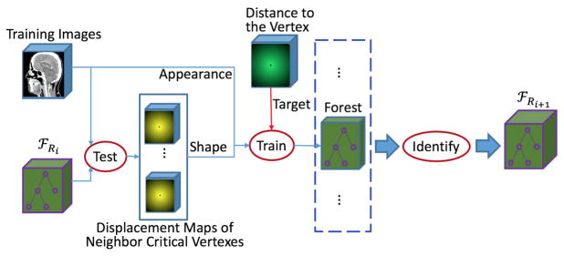
Since local organ shape at a surface point can be determined by the spatial relationship of center surface point to its neighboring surface points, the shape prior information of an organ can thus be learned from the spatial relationships among model vertices. Note that each vector in the 3D displacement map is an estimated displacement vector from the underlying voxel to a specified model vertex. Therefore, the 3D displacement maps of model vertices can provide the spatial relationships among the model vertices. Consequently, once some critical vertices are identified, their learned regression forests 𝔽_j can be used to predict 3D displacement maps, and furthermore these 3D displacement maps can be used to provide shape prior information.

Accordingly, we propose a joint learner of shape and appearance. As shown in Fig. 5, the training procedure is the same as that of the appearance based vertex regression in Section II.E, except for feature extraction and the identification of critical model vertices, as detailed below.

Fig. 5.

Flowchart of joint learner of shape and appearance.

1) Shape and Appearance Feature Extraction

Given both the set of identified critical model vertices ℂ_j = {C_m,j |m = 1, 2, ⋯, M_j} and the set of their corresponding regression forests 𝔽_j = {F_m,j |m = 1, 2, ⋯, M_j}, we can extract not only the appearance features from CT images, but also the shape prior information from the displacement maps predicted using 𝔽_j. To train the regression forest for the m^th model vertex v_m, from critical model vertex set ℂ_j, we first seek a certain number of the closest critical model vertices to v_m (on the mean shape S̄). Then, their corresponding regression forests, a subset of 𝔽_j, are applied to each training CT image to generate the displacement maps. For training each tree in the new regression forests, we use two parts of Haarlike feature sub-space ℱ_sub. The first part is randomly sampled from the Haar-like feature space of intensity image, which capture appearance information. The second part is randomly sampled from the Haar-like feature space of displacement maps (corresponding to those closest critical model vertices), which capture shape prior information.

2) Identification of Critical Model Vertices

In the previous learning steps, some critical model vertices have been already identified. Therefore, in this learning step, we just identify new critical model vertices from the rest of the model vertices.

It is worth noting that the set of critical model vertices ℂ_j identified in the previous learning steps will be re-trained in this training step for refining the predictions. In the previous learning steps, ℂ_j is trained with the shape information extracted on a smaller set ℂ_j−1 or without any shape information (when j = 1). In this training step, the larger set of critical model vertices ℂ_j can provide more elaborate shape prior information and thus can lead to more accurate predictions.

When the training is finished, more model vertices are selected into the current set of critical model vertices ℂ_j+1, and also the set of their corresponding regression forests 𝔽_j+1 are stored for future use.

In the testing stage, the new learned ℂ_j+1 and 𝔽_j+1 are applied to generate displacement maps ${\widehat{\mathbb{Y}}}_{j+1}^{\mathit{test}}$ in the same manner as ℂ₀ and 𝔽₀ (described in Section II.E), except that the input features are not only the appearance features extracted from the intensity image but also the shape features from ${\widehat{\mathbb{Y}}}_j^{\mathit{test}}$ estimated using ℂ_j and 𝔽_j.

G. Hierarchical Vertex Regression

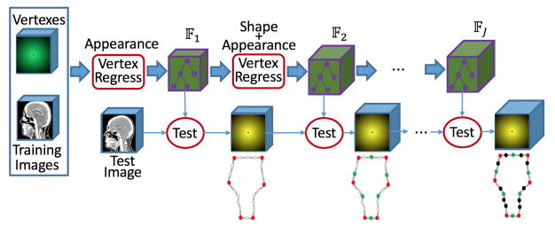
By sequentially linking together an appearance based vertex regressor in Section II.E and several joint learners of shape and appearance in Section II.F, a framework for hierarchical vertex regression can be constructed (Fig. 6).

Fig. 6.

Framework of hierarchical vertex regression.

This framework takes several iterations. The first iteration is an appearance based vertex regressor, which carries out the regression training and also identifies the most critical model vertices based only on the appearance features. The other iterations are the joint learners of shape and appearance, which use not only shape prior but also appearance features to train vertex regressors and identify more critical model vertices.

Given a testing image, the cascaded multilevel regressions {𝔽_j | j = 1, 2, ⋯, J} are successively applied to ultimately generate displacement maps of all critical model vertices ${\widehat{\mathbb{Y}}}_j^{\mathit{test}}$.

In our study, both the number of critical model vertices (identified in each iteration) and the number of iterations used are selected by manually checking the prediction accuracy E_m.

H. Classification Using Displacement Maps as Shape Context

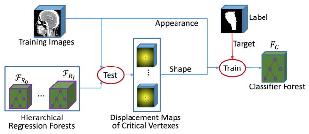
With the hierarchical vertex regression, we obtain the 3D displacement maps of all critical model vertices. In practice, to control the computational cost within a reasonable range, the critical model vertices are often placed sparsely on the organ surface, and thus the segmentation by simply connecting the neighboring critical model vertices to construct organ boundary is not accurate.

To refine the segmentation, we still use the RF based learning procedure, as shown in Fig. 7. In this learning stage, we train a classifier to output binary label for each voxel in the image. The features used to train classifier are the same as those used for joint learner of shape and appearance (Section II.F). Specifically, the previously-trained hierarchical vertex regressors {𝔽_j | j =, 1, 2, ⋯, J} are first applied to each training CT image $I_{\mathit{warp}}^n(n=1,2,\cdots ,N)$ to predict 3D displacement maps for all critical model vertices, i.e., ${\widehat{\mathbb{Y}}}_J=\left\{{\widehat{Y}}_{m,j}^n\mid m=1,2,\cdots ,M;n=1,2,\cdots ,N\right\}$, and then, for each training voxel, both the appearance features from the CT image and the shape features from 𝕐̂_J are extracted for training the classifier F_C, according to the manual segmentation labels such as 1 for target organ and 0 for background.

Fig. 7.

Flowchart of training a classifier for organ segmentation by using displacement maps as shape context.

In the testing stage, for a registered testing CT image $I_{\mathit{warp}}^{\mathit{test}}$, the previously-learned hierarchical vertex regressors {𝔽_j | j = 1, 2, ⋯, J} are sequentially applied to $I_{\mathit{warp}}^{\mathit{test}}$ to generate 3D displacement maps ${\widehat{\mathbb{Y}}}_J^{\mathit{test}}$. Then, the trained classifier F_C is voxel-wisely applied to $I_{\mathit{warp}}^{\mathit{test}}$ to estimate a likelihood map L̂_warp by combining both the appearance features from $I_{\mathit{warp}}^{\mathit{test}}$ and the shape prior from ${\widehat{\mathbb{Y}}}_J^{\mathit{test}}$.

III. Experimental Results

We evaluate our proposed method on segmentation of the brainstem, mandible, left and right parotid glands on a H&N dataset (Section III.A). To carry out quantitative comparison, four measurements (Section III.B) are calculated. The parameter setting for our proposed method is then detailed in Section III.C. We further quantitatively compare our proposed method with 1) the appearance based segmentation method and 2) the conventional deformable model based segmentation method (Section III.D and E). To show the effectiveness of our proposed strategy, i.e., hierarchical vertex regression, quantitative comparison with equal vertex regression is also provided in Section III.F. In Section III.G, the influence of shape correspondence to the performance of our proposed method is discussed. Finally, we list the segmentation results achieved by the state-of-the-art methods and our proposed method in Section III.H, for further comparison.

A. Data Set

We evaluate the performance of our proposed method on a Public Domain Database for Computational Anatomy (PDDCA) (http://www.imagenglab.com/newsite/pddca/). The original CT data is derived from the radiation therapy oncology group (RTOG) 0522 study, a multi-institutional clinical trial led by Ang [54]. The version 1.3 of PDDCA comprises 33 patient CT images from the original set, together with manual segmentations of brainstem, left and right parotid glands, mandible, optic chiasm, and optic nerves (both left and right). The images are contoured based on current best practices as described by RTOG and scientific literature [55].

The image size varies from 257 × 257 × 39 to 257 × 257 × 181. The in-plane resolution ranges from 0.76 mm to 1.25 mm, and the inter-slice thickness ranges from 1.25 mm to 3.0 mm.

In the following experiments, we mainly focus on the segmentation of brainstem, mandible, left parotid gland and right parotid gland from CT images, but our method can also be applied on optic chiasm and optic nerves.

B. Evaluation

In our experiments, we exclude one subject with incomplete region of interest and use two-fold cross validation on the rest 32 subjects to evaluate our method and compare with other methods. We use four measurements to quantitatively assess the accuracy of automatic segmentation, as defined below.

1. Dice Similarity Coefficient (DSC) [56] measures the overlap degree between automatic and manual segmentations.

   $$\mathit{DSC}=\frac{2\Vert {\mathit{Vol}}_{\text{Man}}\cap {\mathit{Vol}}_{\text{Auto}}\Vert }{\Vert {\mathit{Vol}}_{\text{Man}}\Vert +\Vert {\mathit{Vol}}_{\text{Auto}}\Vert }$$ (5)

   where Vol_Man is the voxel set of manually segmented organ and Vol_Auto is the voxel set of automatically segmented organ.

2. Positive Predictive Value (PPV) measures the proportion of correctly segmented volume in the automatic segmentation.

   $$\mathit{PPV}=\frac{\Vert {\mathit{Vol}}_{\text{Man}}\cap {\mathit{Vol}}_{\text{Auto}}\Vert }{\Vert {\mathit{Vol}}_{\text{Auto}}\Vert }$$ (6)
3. Sensitivity (SEN) measures the proportion of correctly segmented volume in the manually segmented organ.

   $$\mathit{SEN}=\frac{\Vert {\mathit{Vol}}_{\text{Man}}\cap {\mathit{Vol}}_{\text{Auto}}\Vert }{\Vert {\mathit{Vol}}_{\text{Man}}\Vert }$$ (7)
4. Average Surface Distance (ASD) measures the average distance between the surface of automatically segmented organ (SEG) and the surface of the manually segmented organ used as ground truth (GT).

   $$\mathit{ASD}=\frac{1}{2}\left\{\frac{{\sum }_{z\in \mathit{SEG}}d(z,GT)}{\mid \mathit{SEG}\mid }+\frac{{\sum }_{u\in GT}d(u,\mathit{SEG})}{\mid GT\mid }\right\}$$ (8)

   where d (z, GT) is the minimum distance of voxel z on the automatically segmented organ surface SEG to the voxels on the ground-truth surface GT, d (u, SEG) is the minimum distance of voxel u on the ground-truth surface GT to the voxels on the automatically segmented organ surface SEG, and |·| is the cardinality of a set.

C. Parameter Settings & Computational Time

1) Parameters for Random Forest

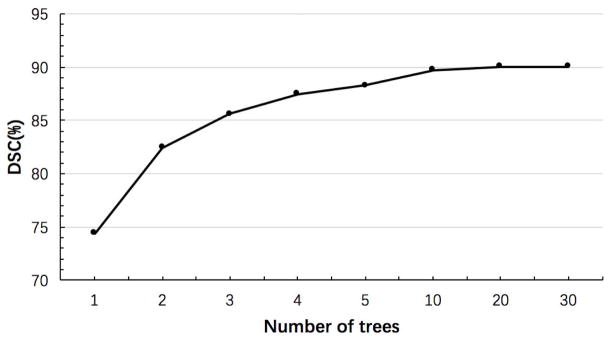
The tree number of the forests is 20. The maximum tree depth is 100. The number of candidate thresholds in each node of a tree in the training stage is 100. The minimum number of training samples in each leaf node is 8. Note that RF parameters have been investigated in many applications [43]–[46], [53], [57]–[60]. Basically, for the number of trees, we find that more trees lead to better results, but also take longer time to do the training. Fig. 8 shows the influence of the number of trees on the segmentation performance. Although the segmentation accuracy increases with the increase of the number of trees, it stops significant improvement after using 20 trees. Thus, we use 20 trees in our experiments. Besides, we also find that the segmentation performance is robust to both the number of thresholds used and also the minimum number of training samples in each leaf node.

Fig. 8.

Influence of the number of trees on brainstem segmentation.

2) Parameters for Haar-Like Features

The patch size and the number of features in Haar-like feature sub-space are 51 × 51 × 51 and 10000, respectively, in the first vertex regression forest (which is used to identify the most critical vertices in Section II.E). In other vertex regression forests (i.e., the joint learner of shape and appearance in Section II.F) and the classification forest (in Section II.H), the patch size is 21 × 21 × 21, the number of features extracted from intensity image is 2000, and the number of features extracted from each displacement map is 30. The sizes of the blocks s₁ and s₂ are randomly selected as 1 or 2 voxels, respectively. The centers of the blocks c₁ and c₂ are uniformly and randomly sampled in the local patch, under the constraint that the blocks should stay within the local patch.

The optimal patch size is related to the complexity of the anatomical structure, which is evaluated in our another work [57] and also in literatures [61], [62]. In this paper, we find that the vertex regression accuracy increases with the increase of patch size when the size is less than a specific value. In the first level R₁, the regression accuracy stop improving with the increase of patch size if the size is greater than about 50. In the other regression level, the regression accuracy keeps steady when the patch size is over 20. This may be due to the case that, in the shape and appearance based regression, the displacement maps generated in the previous level can provide global localization information and thus only local information is needed for precise localization. In the first level R₁, however, since there are no displacement maps can be used, only larger appearance patch can be used to provide the global positioning information.

It is worth noting that a larger patch must associate more features in Haar-like feature sub-space, which will lead to more computational time.

Generally, the number of features is related with the tissue contrast. In our case, since tissue contrast is low in the H&N CT dataset, it is important to extract a large number of features in order to increase the chance of selecting discriminative features.

Note that the voxel values in a ground-truth displacement field are strongly dependent on each other. In other words, once given the displacement vector of a voxel, the displacement vectors of other voxels can be easily computed. However, since the displacement vector of each voxel in the displacement map is predicated independently from nearby voxels, the estimated displacement maps are often noisy. Thus, the voxel values in a predicted displacement map are less dependent on each other than those in a ground-truth displacement field. In our study, we take a compromise solution by sampling a small number of Haar-like features from each predicted displacement map.

3) Other Parameters

The number of vertices on shape surface is determined by the volume of the target organ. A larger organ often needs a large number of vertices for better representation, although this will cause more training and testing time. The number of vertices is 128 for both brainstem and mandible and 64. for both left parotid gland and right parotid gland. The number of critical model vertices identified in each iteration and the number of iterations is selected by manually checking the accuracy of prediction to the training subjects. For brainstem and mandible, which are bigger, the number of iterations is 4 and the numbers of critical model vertices identified in 4 iterations are 16, 32, 64 and 128, respectively. For left and right parotid glands, the number of iterations is 3 and the numbers of critical model vertices identified in 3 iterations are 16, 32 and 64, respectively.

In our study, we use 4-fold cross-validation to identify critical vertex. To evaluate prediction error using Equation (3), the radius of spherical region Ω is set to 20mm, which is determined by cross-validation experiments.

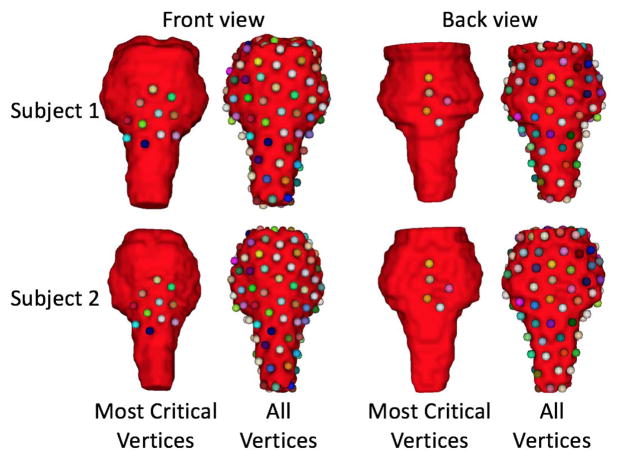
Fig. 9 shows the most critical vertices of two typical subjects for the case of brainstem segmentation. As can be seen in the figure, the 11 most critical vertices are located on the middle-front region of brainstem, and other 5 most critical vertices are located on the mid-posterior region. The main reason is that the organ borders in these region are relatively clear in the H&N CT images.

Fig. 9.

The most critical vertices of 2 typical subjects for the case of brainstem segmentation. The first line shows for Subject 1 and the second line shows for Subject 2. The left two columns show the front view, and the right two columns show the back view. The 16 most critical vertices are shown in the first and third columns. All those 128 vertices are shown in the second and fourth columns.

As described in Section II.F, to extract shape prior information from the predicted displacement maps, we seek a certain number of the closest critical model vertices. Here, the number of the closest critical model vertices is determinded according to the target organ volume. For example, for both the brainstem and mandible, we set it to 7, while, for the parotid gland, we set it to 5.

4) Runtime

The computational cost of the proposed framework is related with the number of trees used, as well as the number of vertices included in the organ shape model. For the number of trees, we find that more trees lead to better results, but also take longer time for the training. For our method, using a 64-bit system computer with an Intel i7-4570 CPU of 3.2GHz and 16GB memory, it takes about 27 mins for training a tree (using 128000 training samples extracted from 16 training images, i.e., 8000 training samples per training image), and about 36 mins to segment brainstem for a new testing subject. It is worth noting that we always need to train all vertices and then select critical vertices in every regression level, so the training time for our hierarchical method is often longer than other non-hierarchical approaches.

D. Comparison With Appearance Based Segmentation

To validate the effectiveness of shape constraint provided by our hierarchical vertex regression, we compare our method with the (only) appearance based segmentation method. In the appearance based segmentation, Haar-like features used for training and testing are extracted only from intensity images. The patch size and the number of features in Haar-like feature sub-space are 51 × 51 × 51 and 10000, respectively.

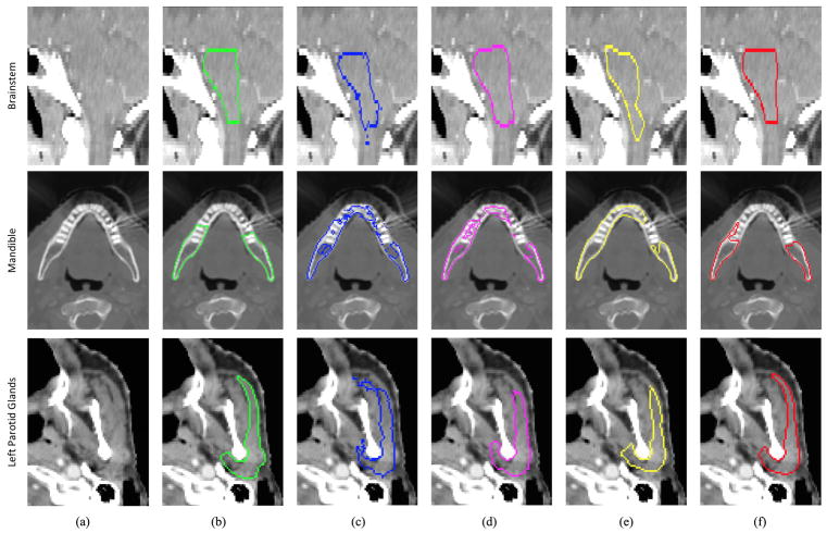
Table I presents a quantitative comparison between the appearance based segmentation method and our proposed method. Fig. 10 (columns c and f) gives visual comparison of the two methods. We can see from these results that the performance of our method is significantly better than that of the appearance based segmentation method. Without any guidance from shape prior, the results by appearance based segmentation are very poor. By using shape prior, our method can more accurately locate organ boundary than the appearance based segmentation method.

TABLE I.

Quantitative Comparison With Appearance Based Segmentation Method

Organ	Method	DSC(%)	PPV(%)	SEN(%)	ASD(mm)
BS	APP	84.4±4.2	83.4±7.3	86.1±6.1	1.76±0.76
	PR	90.3±3.8	90.5±4.0	90.4±3.7	0.91±0.32
MA	AP	89.1±5.7	90.1±2.8	88.5±6.3	1.26±1.16
	PR	94.4±1.3	94.4±2.3	94.5±2.3	0.43±0.12
LP	AP	78.5±5.6	79.6±9.5	77.6±7.5	2.08±0.50
	PR	82.3±5.2	83.6±7.0	82.3±9.9	1.85±0.93
RP	AP	78.1±5.9	76.7±9.2	80.1 ±7.4	2.31±0.58
	PR	82.9±6.1	83.7±6.9	83.3±9.8	1.81±0.63

BS - Brainstem; MA - Mandible; LP - Left Parotid Gland; RP - Right Parotid Gland. AP - Appearance Based Segmentation; PR - Proposed Method.

Fig. 10.

Visual comparison of performances of different segmentation methods. The first row shows a sagittal CT slice of the brainstem. The second row shows an axial slice of the mandible. The third row shows an axial slice of the left parotid gland. The six columns in each row show the original CT slice and five segmentation results (in contours) overlaid on the original CT slice. Contours with different colors denote the results of different methods: green -ground truth; blue - appearance based method; pink - conventional shape model method [19]; yellow – equal vertex regression based method; red - proposed hierarchical vertex regression based method.

E. Comparison With Conventional Deformable Model

To show the effectiveness of hierarchical vertex regression, we compare it with a conventional deformable model proposed in the literature [37]. In that method, a 3D boundary displacement map and an organ likelihood map are first estimated by a multi-task RF with auto-context. Then, a mean shape model sequentially translates, rigidly rotates, and affine transforms under the guidance from the boundary displacement map. Finally, the conventional local search strategy is used to refine the shape model based on the organ likelihood map provided by the image classifier. This method was used to segment the male pelvic organs from CT image and gained high performance.

Table II shows the segmentation accuracies obtained by the boundary regression based deformable method and our hierarchical vertex regression based segmentation method. Fig. 10 (columns (d) and (f)) gives visual comparison of the two methods. We can see that our method achieves more accurate segmentation for the four organs. The reason is that, in our method, the use of both the strategy of hierarchical vertex regression and the mechanism of joint learning of shape and appearance allows more accurate vertex regressions. Moreover, in each iteration, the locations of model vertices are always implicitly moved to their most probable positions, guided by both the shape prior from the neighboring model vertices and the appearance features from intensity image. On the other hand, for the boundary regression based deformable method, its last refinement step just allows local search for each vertex of deformable model along the normal direction, to find the new position with the maximum likelihood gradient. However, the ground-truth position of model vertex is likely not exactly on the normal direction, which leads to segmentation error.

TABLE II.

Quantitative Comparison With Conventional Deformable Model

Organ	Method	DSC(%)	PPV(%)	SEN(%)	ASD(mm)
BS	DM	86.2±4.1	85.5±8.2	87.5±5.7	1.45±0.56
	PR	90.3±3.8	90.5±4.0	90.4±3.7	0.91±0.32
MA	DM	92.9±2.2	93.4±2.4	92.6±4.3	0.74±0.52
	PR	94.4±1.3	94.4±2.3	94.5±2.3	0.43±0.12
LP	DM	80.2±6.1	80.5±10.9	81.4±6.9	1.90±0.49
	PR	82.3±5.2	83.6±7.0	82.3±9.9	1.85±0.93
RP	DM	80.2±5.4	80.2±10.5	81.8±7.6	1.97±0.49
	PR	82.9±6.1	83.7±6.9	83.3±9.8	1.81±0.63

BS - Brainstem; MA - Mandible; LP - Left Parotid Gland; RP - Right Parotid Gland. DM - Conventional Deformable Model; PR - Proposed Method.

F. Hierarchical Versus Equal Vertex Regression

One advantage of our method is to hierarchically estimate the locations of critical model vertices with the guidance of the critical model vertices located previously. To evaluate the effectiveness of this strategy, the comparison experiment for hierarchical and equal vertex regressions is also conducted.

In the case of equal vertex regression, we do not identify critical model vertex, but use all the model vertices equally in guiding the segmentation. In the training stage, for each vertex of the shape model, an appearance based regressor is first learned; then, all the trained regressors are applied to all the training CT images to generate the 3D displacement maps, which are finally used as shape context to train an organ classifier. In the testing stage, given a testing CT image, for each vertex of the shape model, a 3D displacement map is first predicted, and then all the 3D displacement maps are used as shape context and inputted to the trained classifier for segmentation.

Table III presents the results of this experiment. Fig. 10 (columns (e) and (f)) also gives visual comparison of the two methods. We can see that the hierarchical vertex regression can significantly improve the segmentation accuracy.

TABLE III.

Quantitative Comparison With Equal Vertex Regression Based Segmentation Method

Organ	Method	DSC(%)	PPV(%)	SEN(%)	ASD(mm)
BS	EVR	84.8±6.3	85.5±8.3	85.1±9.2	1.68±1.37
	PR	90.3±3.8	90.5±4.0	90.4±3.7	0.91±0.32
MA	EVR	92.7±2.8	93.3±3.0	92.3±4.7	0.98±0.98
	PR	94.4±1.3	94.4±2.3	94.5±2.3	0.43±0.12
LP	EVR	80.6±8.1	80.6±13.5	82.7±8.2	1.91 ±0.78
	PR	82.3±5.2	83.6±7.0	82.3±9.9	1.85±0.93
RP	EVR	81.4±9.9	82.6±14.5	81.9±6.9	1.94±0.90
	PR	82.9±6.1	83.7±6.9	83.3±9.8	1.81±0.63

BS - Brainstem; MA - Mandible; LP - Left Parotid Gland; RP - Right Parotid Gland. EVR – Equal Vertex Regression; PR - Proposed Method.

G. Influence of Shape Correspondence

We can also see from the Tables I and II that the segmentation improvement by our method varies from organ to organ. The main reason is that the performance of our method is dependent on the accuracy of shape correspondences detected across training subjects in the training dataset. Only the vertices with accurately-detected correspondences across training subjects can be accurately located by the regressor in the application stage, thus leading to accurate organ segmentation.

In our experiments, a public software named “ShapeWorks” (https://www.sci.utah.edu/software/shapeworks.html) is used to construct shape correspondence. This software uses a method, called entropy-based particle systems, for shape correspondence detection [41], [42].

For the brainstem and mandible, their organ shapes in different training subjects are similar to each other, and “ShapeWorks” can construct better vertex correspondences. Thus, when segmenting the brainstem, by using the hierarchical guidance of critical model vertices, our method overcomes the effect of low tissue contrast in the CT images and gains obviously more accurate performance than both the appearance based method and the conventional deformable model. Also, when segmenting the mandible, although the conventional deformable model can achieve good results due to clear boundaries of bony tissue, our method still gains 1.4% improvement in DSC.

For the left and right parotid glands, due to huge shape difference across individual subjects, “ShapeWorks” cannot construct good correspondences across different subjects and thus the regressors cannot locate critical vertices accurately. Thus, due to insufficient guidance from these critical model vertices, our method achieves just a small improvement in segmentation of parotid glands.

H. Comparison With State-of-the-art Methods

Since different methods were validated by different datasets, metrics and target organs, as well as none of them published their source codes or binary executables, a fair comparison with other methods is difficult. We compare our method with 6 methods [29], [63]–[67] evaluated on the dataset PDDCA in the Table IV. Note that the method [29] was just evaluated on a subset of dataset PDDCA with only 18 high-resolution CT images. The method [63] won the MICCAI 2015 Head and Neck Auto Segmentation Grand Challenge. The comparison results show that our method obtains the best performance, compared to all these state-of-the-art methods.

TABLE IV.

Comparison Between State-of-the-Art Method and Our Proposed Methods

Organ	Method	DSC(%)
Brain Stem	Mannion [62]	88±3
	Arteaga [65]	86±5
	Albrecht [63]	85±5
	Chen [66]	80±7
	Fritscher [28]	86±(−)
	Proposed	90±4
Mandible	Mannion [62]	91±2
	Arteaga [65]	93±2
	Albrecht [63]	88±6
	Chen [66]	92±2
	Aghdasi [64]	79±5
	Proposed	94±1
Parotid Glands (Left and Right)	Mannion [62]	82±1
	Arteaga [65]	76±8
	Albrecht [63]	82±5
	Chen [66]	81±5
	Fritscher [28]	82±(−)
	Proposed	83±6

IV. Conclusions

In this paper, we have proposed a hierarchical vertex regression based segmentation method to segment OARs from H&N CT images for radiotherapy planning. Specifically, by developing three novel strategies, i.e., hierarchical critical model vertex identification, joint learning of shape and appearance, and hierarchical vertex regression, our method can essentially solve the drawback of sensitivity to shape initialization in the conventional deformable models. Experimental results also show that our proposed method achieves higher segmentation accuracy than both the appearance based method and the conventional deformable model, and also obtains competitive performance compared to the state-of-the-art methods.

However, there are still two potential issues with our proposed method. 1) The shape model is constructed based on the shape correspondences detected across all atlases, and thus our proposed method is heavily dependent on the accuracy of the shape correspondence detection method used. 2) The shape prior information is extracted from the predicted displacement maps of the closest critical model vertices. Consequently, the prediction accuracy current critical vertices affects the subsequent regression or classification. Although our mechanism for identifying critical vertices works well in our current database, it is still possible that, in the extreme cases, the testing image is noisy at the position of certain critical vertex, thus leading to poor prediction of the critical vertex. The prediction error will propagate and eventually lead to poor segmentation. In the future, we will do some research to automatically identify those poorly-predicted critical vertices and then minimize their influences on the subsequent segmentation steps.

Besides, the computational cost of our proposed method is also intensive. We expect that the parallel computing techniques can be used to reduce the computational time of our proposed method.

In this work, the implementation of our idea is based on random forest, incorporated with Haar-like features. Other handcrafted features may also be used, which will be investigated in our future work. In addition, we will also investigate deep learning frameworks, such as FCN, U-Net and GANs, as well as deep shape features [68], to automatically learn effective features and incorporate them into our model.

Biographies

Zhensong Wang received the B.S. and M.S. degrees in automatic control, control theory and control engineering from the University of Electronic Science and Technology of China (UESTC), Chengdu, China, in 1998 and 2003, respectively, where he is currently pursuing the Ph.D. degree with the School of Automation Engineering. He was a Visiting Scholar with the University of North Carolina at Chapel Hill from 2015 to 2016. He is also an Instructor with UESTC. His research interests include machine learning and medical image analysis.

Lifang Wei received the bachelor’s degree in electronic communication engineering from Xi’an Shiyou University, Xi’an, China, in 2005, the master’s degree in biomedical engineering from Northwest Polytechnical University, Xi’an, in 2008, and the Ph.D. degree in communication and information system from Fuzhou University, Fuzhou, China, in 2013. She is currently an Instructor with the College of Computer and Information, Fujian Agriculture and Forestry University, Fuzhou. Her research interests focus on computer vision and image processing.

Li Wang is currently a Research Assistant Professor with the University of North Carolina at Chapel Hill, USA. He is involved in the medical image analysis field with Prof. D. Shen. His research interests focus on image segmentation, image registration, cortical surface analysis, machine learning, and their applications to normal early brain development and disorders.

Yaozong Gao received the Ph.D. degree from the Department of Computer Science, University of North Carolina at Chapel Hill. He was a Computer Vision Researcher with Apple. He is currently directing the Deep Learning Group, United Imaging, China. He has published over 90 papers in the international journals and conferences, such as MICCAI, TMI, and MIA. His research interests include machine learning, computer vision and medical image analysis. He received the Best Paper Award at the Machine Learning and Medical Imaging Workshop of the MICCAI conference.

Wufan Chen received the B.S. and M.S. degrees in applied mathematics and computational fluid dynamics from the Peking University of Aeronautics and Astronautics, China, in 1975 and 1981, respectively. From 1981 to 1987, he was with the School of Aerospace, National University of Defense Technology, China. From 1987 to 2004, he was with the Department of Training, First Military Medical University, China. Since 2004, he has been with Southern Medical University, China, where he currently holds the rank of a Professor with the School of Biomedical Engineering and the Director of the Key Laboratory for Medical Image Processing of Guangdong province. His research focuses on the medical imaging and medical image analysis.

Dinggang Shen is currently a Jeffrey Houpt Distinguished Investigator and a Professor with the Radiology, Biomedical Research Imaging Center (BRIC), Computer Science, and Biomedical Engineering, University of North Carolina at Chapel Hill. He also directs the Center for Image Analysis and Informatics, the Image Display, Enhancement, and Analysis Laboratory, Department of Radiology, and the medical image analysis core at BRIC. He was a Tenure-Track Assistant Professor with the University of Pennsylvanian and a Faculty Member with Johns Hopkins University. He has published over 800 papers in international journals and conference proceedings. His research interests include medical image analysis, computer vision, and pattern recognition. He is a fellow of the American Institute for Medical and Biological Engineering. He serves as an Editorial Board Member for eight international journals and served on the Board of Directors for The Medical Image Computing and Computer Assisted Intervention Society from 2012 to 2015.

References

- 1.O’Rorke MA, Ellison MV, Murray LJ, Moran M, James J, Anderson LA. Human papillomavirus related head and neck cancer survival: A systematic review and meta-analysis. Oral Oncol. 2012 Dec;48(12):1191–1201. doi: 10.1016/j.oraloncology.2012.06.019. [DOI] [PubMed] [Google Scholar]
- 2.Brouwer CL, et al. 3D variation in delineation of head and neck organs at risk. Radiat Oncol. 2012 Mar;7(1):32. doi: 10.1186/1748-717X-7-32. [DOI] [PMC free article] [PubMed] [Google Scholar]
- 3.Rasch C, et al. Irradiation of paranasal sinus tumors, a delineation and dose comparison study. Int J Radiat Oncol. 2002 Jan;52(1):120–127. doi: 10.1016/s0360-3016(01)01751-5. [DOI] [PubMed] [Google Scholar]
- 4.Nelms BE, Tomé WA, Robinson G, Wheeler J. Variations in the contouring of organs at risk: Test case from a patient with oropharyngeal cancer. Int J Radiat Oncol. 2012 Jan;82(1):368–378. doi: 10.1016/j.ijrobp.2010.10.019. [DOI] [PubMed] [Google Scholar]
- 5.Street E, et al. Automated volume analysis of head and neck lesions on CT scans using 3D level set segmentation. Med Phys. 2007 Nov;34(11):4399–4408. doi: 10.1118/1.2794174. [DOI] [PMC free article] [PubMed] [Google Scholar]
- 6.Han X, et al. Medical Image Computing and Computer-Assisted. New York, NY, USA: Springer; 2008. Atlas-based auto-segmentation of head and neck CT images; pp. 434–441. [DOI] [PubMed] [Google Scholar]
- 7.Levendag PC, et al. Atlas based auto-segmentation of CT images: Clinical evaluation of using auto-contouring in high-dose, high-precision radiotherapy of cancer in the head and neck. Int J Radiat Oncol. 2008 Sep;72(1):S401. [Google Scholar]
- 8.Sims R, et al. A pre-clinical assessment of an atlas-based automatic segmentation tool for the head and neck. Radiotherapy Oncol. 2009 Dec;93(3):474–478. doi: 10.1016/j.radonc.2009.08.013. [DOI] [PubMed] [Google Scholar]
- 9.Chen A, Deeley MA, Niermann KJ, Moretti L, Dawant BM. Combining registration and active shape models for the automatic segmentation of the lymph node regions in head and neck CT images. Med Phys. 2010 Dec;37(12):6338–6346. doi: 10.1118/1.3515459. [DOI] [PMC free article] [PubMed] [Google Scholar]
- 10.Fortunati V, et al. Tissue segmentation of head and neck CT images for treatment planning: A multiatlas approach combined with intensity modeling. Med Phys. 2013 Jul;40(7):071905. doi: 10.1118/1.4810971. [DOI] [PubMed] [Google Scholar]
- 11.Long J, Shelhamer E, Darrell T. Proc CVPR. Boston, MA, USA: 2015. Fully convolutional networks for semantic segmentation; pp. 3431–3440. [DOI] [PubMed] [Google Scholar]
- 12.Ronneberger O, Fischer P, Brox T. Medical Image Computing and Computer-Assisted Intervention—MICCAI. Munich, Germany: Springer; 2015. U-Net: Convolutional networks for biomedical image segmentation; pp. 234–241. [Google Scholar]
- 13.Goodfellow IJ, et al. Generative adversarial nets. Proc. NIPS; Montreal, QC, Canada. 2014. pp. 2672–2680. [Google Scholar]
- 14.Papandreou G, Chen L-C, Murphy KP, Yuille AL. Weakly- and semi-supervised learning of a deep convolutional network for semantic image segmentation. Proc. ICCV; Santiago, Chile. Dec. 2015; pp. 1742–1750. [Google Scholar]
- 15.Chen L-C, Papandreou G, Kokkinos I, Murphy K, Yuille AL. Semantic image segmentation with deep convolutional nets and fully connected CRFs. 2014 doi: 10.1109/TPAMI.2017.2699184. [Online]. Available: https://arxiv.org/abs/1412.7062. [DOI] [PubMed]
- 16.Li Q, Cai W, Wang X, Zhou Y, Feng DD, Chen M. Medical image classification with convolutional neural network. Proc. ICARCV; Singapore. Dec. 2014; pp. 844–848. [Google Scholar]
- 17.Tajbakhsh N, et al. Convolutional neural networks for medical image analysis: Full training or fine tuning? IEEE Trans Med Imag. 2016 May;35(5):1299–1312. doi: 10.1109/TMI.2016.2535302. [DOI] [PubMed] [Google Scholar]
- 18.Prasoon A, Petersen K, Igel C, Lauze F, Dam E, Nielsen M. Medical Image Computing and Computer-Assisted Intervention—MICCAI. Nagoya, Japan: Springer; 2013. Deep feature learning for knee cartilage segmentation using a triplanar convolutional neural network; pp. 246–253. [DOI] [PubMed] [Google Scholar]
- 19.Zhang H, Zhang S, Li K, Metaxas DN. Robust shape prior modeling based on Gaussian–Bernoulli restricted Boltzmann machine. Proc. IEEE Int. Symp. Biomed. Imag; Beijing, China. Apr./May 2014; pp. 270–273. [Google Scholar]
- 20.Wang G, Zhang S, Li F, Gu L. A new segmentation framework based on sparse shape composition in liver surgery planning system. Med Phys. 2013 May;40(5):051913. doi: 10.1118/1.4802215. [DOI] [PMC free article] [PubMed] [Google Scholar]
- 21.Uzunbaş MG, Chen C, Zhang ST, Pohl KM, Li K, Metaxas D. Medical Image Computing and Computer-Assisted Intervention—MICCAI. Nagoya, Japan: Springer; 2013. Collaborative multi organ segmentation by integrating deformable and graphical models; pp. 157–164. [DOI] [PMC free article] [PubMed] [Google Scholar]
- 22.Zhang ST, Zhan Y, Zhou Y, Uzunbas M, Metaxas DN. Medical Image Computing and Computer-Assisted Intervention—MICCAI. Nice, France: Springer; 2012. Shape prior modeling using sparse representation and online dictionary learning; pp. 435–442. [DOI] [PubMed] [Google Scholar]
- 23.Uzunbaş MG, Zhang S, Pohl KM, Metaxas D, Axel L. Segmentation of myocardium using deformable regions and graph cuts. Proc. IEEE Int. Symp. Biomed. Imag; Barcelona, Spain. May 2012; pp. 254–257. [DOI] [PMC free article] [PubMed] [Google Scholar]
- 24.Chen X, Udupa JK, Bagci U, Zhuge Y, Yao J. Medical image segmentation by combining graph cuts and oriented active appearance models. IEEE Trans Image Process. 2012 Apr;21(4):2035–2046. doi: 10.1109/TIP.2012.2186306. [DOI] [PMC free article] [PubMed] [Google Scholar]
- 25.Li G, Chen X, Shi F, Zhu W, Tian J, Xiang D. Automatic liver segmentation based on shape constraints and deformable graph cut in CT images. IEEE Trans Image Process. 2015 Dec;24(12):5315–5329. doi: 10.1109/TIP.2015.2481326. [DOI] [PubMed] [Google Scholar]
- 26.Zhu LJ, et al. A complete system for automatic extraction of left ventricular myocardium from CT images using shape segmentation and contour evolution. IEEE Trans Image Process. 2014 Mar;23(3):1340–1351. doi: 10.1109/TIP.2014.2300751. [DOI] [PMC free article] [PubMed] [Google Scholar]
- 27.Pujadas ER, Reisert M. Shape-based normalized cuts using spectral relaxation for biomedical segmentation. IEEE Trans Image Process. 2014 Jan;23(1):163–170. doi: 10.1109/TIP.2013.2287604. [DOI] [PubMed] [Google Scholar]
- 28.Zhu L, Gao Y, Yezzi A, Tannenbaum A. Automatic segmentation of the left atrium from MR images via variational region growing with a moments-based shape prior. IEEE Trans Image Process. 2013 Dec;22(12):5111–5122. doi: 10.1109/TIP.2013.2282049. [DOI] [PMC free article] [PubMed] [Google Scholar]
- 29.Fritscher KD, Peroni M, Zaffino P, Spadea MF, Schubert R, Sharp G. Automatic segmentation of head and neck CT images for radiotherapy treatment planning using multiple atlases, statistical appearance models, and geodesic active contours. Med Phys. 2014 May;41(5):051910. doi: 10.1118/1.4871623. [DOI] [PMC free article] [PubMed] [Google Scholar]
- 30.Feng Q, Foskey M, Chen W, Shen D. Segmenting CT prostate images using population and patient-specific statistics for radiotherapy. Med Phys. 2010 Aug;37(8):4121–4132. doi: 10.1118/1.3464799. [DOI] [PMC free article] [PubMed] [Google Scholar]
- 31.Chen S, Lovelock DM, Radke RJ. Segmenting the prostate and rectum in CT imagery using anatomical constraints. Med Image Anal. 2011 Feb;15(1):1–11. doi: 10.1016/j.media.2010.06.004. [DOI] [PubMed] [Google Scholar]
- 32.Lu C, et al. Medical Image Computing and Computer-Assisted Intervention—MICCAI. Nice, France: Springer; 2012. Precise segmentation of multiple organs in CT volumes using learning-based approach and information theory; pp. 462–469. [DOI] [PubMed] [Google Scholar]
- 33.Li W, Liao S, Feng Q, Chen W, Shen D. Learning image context for segmentation of the prostate in CT-guided radiotherapy. Phys Med Biol. 2012 Mar;57(5):1283–1308. doi: 10.1088/0031-9155/57/5/1283. [DOI] [PMC free article] [PubMed] [Google Scholar]
- 34.Zhou H, Lam K-M, He X. Shape-appearance-correlated active appearance model. Pattern Recognit. 2016 Aug;56:88–99. [Google Scholar]
- 35.Cootes TF, Taylor CJ, Cooper DH, Graham J. Active shape models—Their training and application. Comput Vis Image Understand. 1995 Jan;61(1):38–59. [Google Scholar]
- 36.Shao Y, Gao Y, Wang Q, Yang X, Shen D. Locally-constrained boundary regression for segmentation of prostate and rectum in the planning CT images. Med Image Anal. 2015 Dec;26(1):345–356. doi: 10.1016/j.media.2015.06.007. [DOI] [PMC free article] [PubMed] [Google Scholar]
- 37.Gao Y, Lian J, Shen D. Medical Image Computing and Computer-Assisted Intervention—MICCAI. Munich, Germany: Springer; 2015. Joint learning of image regressor and classifier for deformable segmentation of CT pelvic organs; pp. 114–122. [Google Scholar]
- 38.Wu G, Jia H, Wang Q, Shen D. SharpMean: Groupwise registration guided by sharp mean image and tree-based registration. NeuroImage. 2011 Jun;56(4):1968–1981. doi: 10.1016/j.neuroimage.2011.03.050. [DOI] [PMC free article] [PubMed] [Google Scholar]
- 39.Munsell BC, Dalal P, Wang S. Evaluating shape correspondence for statistical shape analysis: A benchmark study. IEEE Trans Pattern Anal Mach Intell. 2008 Nov;30(11):2023–2039. doi: 10.1109/TPAMI.2007.70841. [DOI] [PubMed] [Google Scholar]
- 40.van Kaick O, Zhang H, Hamarneh G, Cohen-Or D. A survey on shape correspondence. Comput Graph Forum. 2011 Sep;30(6):1681–1707. [Google Scholar]
- 41.Oguz I, et al. Entropy-based particle correspondence for shape populations. Int J Comput Assist Radiol Surg. 2016 Jul;11(7):1221–1232. doi: 10.1007/s11548-015-1319-6. [DOI] [PMC free article] [PubMed] [Google Scholar]
- 42.Cates J, Fletcher PT, Styner M, Shenton M, Whitaker R. Shape modeling and analysis with entropy-based particle systems. Proc. Int. Conf. Inf. Process. Med. Imag; Kerkrade, The Netherlands. 2007. pp. 333–345. [DOI] [PMC free article] [PubMed] [Google Scholar]
- 43.Criminisi A, Shotton J, Konukoglu E. Decision forests: A unified framework for classification, regression, density estimation, manifold learning and semi-supervised learning. Found Trends Comput Graph Vis. 2012 Feb;7(2–3):81–227. [Google Scholar]
- 44.Criminisi A, Shotton J, Robertson D, Konukoglu E. Regression forests for efficient anatomy detection and localization in CT studies. Proc. Med. Image Comput. Comput. Assist. Interv. MCV Workshop; Toronto, ON, Canada. 2011. pp. 106–117. [Google Scholar]
- 45.Lindner C, Thiagarajah S, Wilkinson JM, Wallis GA, Cootes TF Consortium TA. Fully automatic segmentation of the proximal femur using random forest regression voting. IEEE Trans Med Imag. 2013 Aug;32(8):1462–1472. doi: 10.1109/TMI.2013.2258030. [DOI] [PubMed] [Google Scholar]
- 46.Cootes TF, Ionita MC, Lindner C, Sauer P. Robust and accurate shape model fitting using random forest regression voting. Proc. Euro. Conf. Comp. Vis; Florence, Italy. 2012. pp. 278–291. [Google Scholar]
- 47.Fanelli G, Dantone M, Gall J, Fossati A, Van Gool L. Random forests for real time 3D face analysis. Int J Comput Vis. 2013 Feb;101(3):437–458. [Google Scholar]
- 48.Gall J, Lempitsky V. Class-specific Hough forests for object detection. Proc. IEEE Comput. Soc. Conf. Comput. Vis. Pattern Recognit; Miami, FL, USA. Jun. 2009; pp. 1022–1029. [Google Scholar]
- 49.Mahapatra D. Analyzing training information from random forests for improved image segmentation. IEEE Trans Image Process. 2014 Apr;23(4):1504–1512. doi: 10.1109/TIP.2014.2305073. [DOI] [PubMed] [Google Scholar]
- 50.Mahapatra D, et al. Automatic detection and segmentation of Crohn’s disease tissues from abdominal MRI. IEEE Trans Med Imag. 2013 Dec;32(12):2332–2347. doi: 10.1109/TMI.2013.2282124. [DOI] [PubMed] [Google Scholar]
- 51.Viola P, Jones M. Rapid object detection using a boosted cascade of simple features. Proc. IEEE Comput. Soc. Conf. Comput. Vis. Pattern Recognit; Kauai, HI, USA. Dec. 2001; pp. 511–518. [Google Scholar]
- 52.Viola P, Jones MJ. Robust real-time face detection. Int J Comput Vis. 2004 May;57(2):137–154. [Google Scholar]
- 53.Gao Y, Shao Y, Lian J, Wang AZ, Chen RC, Shen D. Accurate segmentation of CT male pelvic organs via regression-based deformable models and multi-task random forests. IEEE Trans Med Imag. 2016 Jun;35(6):1532–1543. doi: 10.1109/TMI.2016.2519264. [DOI] [PMC free article] [PubMed] [Google Scholar]
- 54.Ang KK, et al. Randomized phase III trial of concurrent accelerated radiation plus cisplatin with or without cetuximab for stage III to IV head and neck carcinoma: RTOG 0522. J Clin Oncol. 2014 Sep;32(27):2940–2950. doi: 10.1200/JCO.2013.53.5633. [DOI] [PMC free article] [PubMed] [Google Scholar]
- 55.van de Water TA, Bijl HP, Westerlaan HE, Langendijk JA. Delineation guidelines for organs at risk involved in radiation-induced salivary dysfunction and xerostomia. Radiotherapy Oncol. 2009 Dec;93(3):545–552. doi: 10.1016/j.radonc.2009.09.008. [DOI] [PubMed] [Google Scholar]
- 56.Dice LR. Measures of the amount of ecologic association between species. Ecology. 1945 Jul;26(3):297–302. [Google Scholar]
- 57.Wang L, et al. LINKS: Learning-based multi-source integration framework for segmentation of infant brain images. NeuroImage. 2015 Mar;108:160–172. doi: 10.1016/j.neuroimage.2014.12.042. [DOI] [PMC free article] [PubMed] [Google Scholar]
- 58.Gao Y, Shen D. Collaborative regression-based anatomical landmark detection. Phys Med Biol. 2015 Dec;60(24):9377–9401. doi: 10.1088/0031-9155/60/24/9377. [DOI] [PMC free article] [PubMed] [Google Scholar]
- 59.Zhang J, Gao Y, Wang L, Tang Z, Xia JJ, Shen D. Automatic craniomaxillofacial landmark digitization via segmentation-guided partially-joint regression forest model and multiscale statistical features. IEEE Trans Biomed Eng. 2016 Sep;63(9):1820–1829. doi: 10.1109/TBME.2015.2503421. [DOI] [PMC free article] [PubMed] [Google Scholar]
- 60.Huynh T, et al. Estimating CT image from MRI data using structured random forest and auto-context model. IEEE Trans Med Imag. 2016 Jan;35(1):174–183. doi: 10.1109/TMI.2015.2461533. [DOI] [PMC free article] [PubMed] [Google Scholar]
- 61.Coupé P, Manjón JV, Fonov V, Pruessner J, Robles M, Collins DL. Patch-based segmentation using expert priors: Application to hippocampus and ventricle segmentation. NeuroImage. 2011;54(2):940–954. doi: 10.1016/j.neuroimage.2010.09.018. [DOI] [PubMed] [Google Scholar]
- 62.Tong T, Wolz R, Coupé P, Hajnal JV, Rueckert D. Segmentation of MR images via discriminative dictionary learning and sparse coding: Application to hippocampus labeling. NeuroImage. 2013 Aug;76:11–23. doi: 10.1016/j.neuroimage.2013.02.069. [DOI] [PubMed] [Google Scholar]
- 63.Mannion-Haworth R, Bowes M, Ashman A, Guillard G, Brett A, Vincent G. Fully automatic segmentation of head and neck organs using active appearance models. MIDAS J. 2016 Jan; [Online]. Available: http://www.midasjournal.org/browse/publication/967.
- 64.Albrecht T, Gass T, Langguth C, Lüthi M. Multi atlas segmentation with active shape model refinement for multi-organ segmentation in head and neck cancer radiotherapy planning. MIDAS J. 2015 Dec; [Online]. Available: http://www.midasjournal.org/browse/publication/968.
- 65.Aghdasi N, Li Y, Berens AY, Moe K, Hannaford B. Automatic mandible segmentation on CT images using prior anatomical knowledge. MIDAS J. 2016 Mar; [Online]. Available: http://www.midasjournal.org/browse/publication/971.
- 66.Arteaga MO, Peña DC, Dominguez GC. Head and neck auto segmentation challenge based on non-local generative models. MIDAS J. 2016 Oct; [Online]. Available: http://www.midasjournal.org/browse/publication/965.
- 67.Chen A, Dawant B. A multi-atlas approach for the automatic segmentation of multiple structures in head and neck CT images. MIDAS J. 2016 Feb; [Online]. Available: http://www.midasjournal.org/browse/publication/964.
- 68.Xie J, Fang Y, Zhu F, Wong E. Deepshape: Deep learned shape descriptor for 3D shape matching and retrieval. Proc. CVPR; Boston, MA, USA. Jun. 2015; pp. 1275–1283. [Google Scholar]