TRAFIC: Fiber Tract Classification Using Deep Learning

Abstract

We present TRAFIC, a fully automated tool for the labeling and classification of brain fiber tracts. TRAFIC classifies new fibers using a neural network trained using shape features computed from previously traced and manually corrected fiber tracts. It is independent from a DTI Atlas as it is applied to already traced fibers. This work is motivated by medical applications where the process of extracting fibers from a DTI atlas, or classifying fibers manually is time consuming and requires knowledge about brain anatomy. With this new approach we were able to classify traced fiber tracts obtaining encouraging results. In this report we will present in detail the methods used and the results achieved with our approach.

1. INTRODUCTION

The white matter (WM) contains millions of nerve fibers that connect different regions in the brain. These nerve fibers can be grouped in bundles according to criteria such as location or the brain regions they link. Fiber bundles have specific connectivity roles in the brain. Therefore, identifying these bundles can help us reveal connectivity abnormalities that are characteristic of some diseases and/or behavioral disorders in humans.

DWI or Diffusion Weighted Imaging is a form of Magnetic Resonance Imaging (MRI) that measures the rate of water motion inside a structure of interest or tissue.¹ In Diffusion Tensor Imaging (DTI), a tensor is calculated that best fits the DWI data at each voxel. If an eigen-decomposition is done to each tensor, the main eigenvector represents the most likely direction of water flow at a particular voxel. With a DTI of the brain, it is possible to represent the white matter tract orientation at each voxel.²

Complete fiber tracts are generated using tractography algorithms. These algorithms require user input to define a starting seed point, and also the definition of a stopping criteria. Nevertheless, in most cases, the tracing goes beyond the structure of interest and a manual clean up step of the traced fiber is needed. The whole process requires technical and anatomical knowledge. Moreover, tracing fibers in brain structures is subject to a certain bias related to the person that extracts the fiber and is a time-consuming operation.

An earlier attempt to automate the tracing and cleaning of fibers was done with AutoTract.³ Autotract uses a reference DTI atlas with a set of traced fiber bundles to initialize a tractography algorithm in a target DTI. A cleaning procedure is guided using binary masks and morphological operations on the resulting fiber bundles. Unfortunately, Autotract has some disadvantages as the results of the tracing and cleaning are dependent on the quality of the registration of the reference atlas and target DTI image. Additionally, the cleaning procedure often fails to remove unwanted fibers, or removes fibers that belong to the structure of interest.

To address these issues, we present TRAFIC, a tool developed to automate the tracing and classification of fibers. TRAFIC seeks to accelerate hypothesis testing in neuroscience studies and will be part of the UNC NA-MIC DTI framework.⁴

TRAFIC trains a deep neural network to reject unwanted fiber tracts. In contrast to Autotract, TRAFIC learns shape features that are unique for each fiber bundle.

The following section gives details about our neural network and explains the pre-processing steps required to prepare the data for training and classification.

2. MATERIALS

2.1 Subjects

DTI data from a total of 685 subjects were collected across three age groups including 429 twin (173 monozy-gotic, 256 dizygotic) and 256 non-twin subjects (male/female: 366/319, Caucasian/African American/Asian: 525/146/14). There were 535 subjects with analyzable DTI scans at birth, 322 at 1 y, and 244 at 2 y; among 322 subjects with usable scans at age 1 y, 217 (67%) were included at birth; of the 244 with usable scans at age 2 y,164(67%) were included at birth and 134 (55%) were included at age 1 y.

2.2 Image acquisition

The MRI data were acquired on a 3T Siemens Allegra head- only scanner (Siemens Medical System), comprising 86% of the neonates, 82% of the 1-y-olds, and 77% of the 2-y-olds in the present study. For earlier Allegra diffusion-weighted imaging (DWI) data, a single-shot echo-planar imaging spin-echo sequence was used with the following parameters: Repetition Time (TR)/Echo Time (TE) = 5, 200/73ms, slice thickness = 2mm, and in-plane resolution = 2 * 2mm², with a total of 45 slices for six directions using b value = 1, 000s/mm² and 1 baseline image (b value = 0) per sequence, repeated five times total to improve signal-to-noise. For the remaining Allegra DWI data, 42 directions of diffusion sensitization were acquired with a b value of 1, 000s/mm² in addition to seven images with no diffusion weighting for reference. The parameters were as follows: TR/TE/Flip angle = 7, 680/82/90°, slice thickness = 2mm, and in-plane resolution = 2 * 2mm², with a total of 60 to 72 slices.

2.3 Atlas generation

Image Quality Control (QC) is done using DTIPrep.⁵ After this initial QC process, a population atlas is generated using DTI-AtlasBuilder.^4,6 The atlas allows comparison of diffusion properties in the population of diffusion tensor images. The goal of the atlas building procedure is to provide spatial normalization for analysis of diffusion values at corresponding locations. DTI-AtlasBuilder is an iterative procedure that will refine the registrations for each subject. Starting with linear transformations (affine) and moving towards non linear (diffeomorphic).

DTI-AtlasBuilder takes the tensor image I and the corresponding Fractional Anisotropy F A image as input. A feature image C is computed using the maximum eigenvalue of the Hessian of the F A image. The Hessian is computed by convolution of the F A and a set of Gaussian (second derivative) kernels. The σ value for the kernel is chosen empirically (smaller value for smaller brains, i.e., smaller for neonates than adults).

The feature image C is used for the atlas building procedure described in.⁷ Image C is a good detector of major fiber bundles which occur as tubular or sheet-like structures. By guiding the registration procedure with these images we achieve better correspondence of bundles across the population.

The transformations generated during this process are concatenated and a global displacement field is generated for each subject. Each subject is transformed into the atlas space. However, to re-sample the tensors, Riemannian methods are used to preserve their shape and orientation.⁸ The transformed images are averaged using the Log-Euclidean method to produce a tensor atlas. The tensor atlas provides an image with improved signal-to-noise ratio (SNR) that is used to create template fiber tracts. These template bundles are traced and validated by experts. In the following section, the traced fiber bundles will be used to train the neural network.

3. METHODS

3.1 Pre-processing fibers

Tractography algorithms produce fibers with different length and number of points, therefore, it is necessary to re-sample them to contain the same number of elements independent of their length. This will facilitate the design and training of the deep neural network. Once the number of points across fibers is uniform, a set of features is computed for each fiber at each point. In general, the input data will have n_pt * n_feat where n_pt is the fixed number of points and n_feat is the number of features computed for each point in the fiber.

The following features are computed for each fiber: curvature, torsion and euclidean distances to a certain number of landmarks. These features were selected because they are purely geometric and they do not depend on the position nor the orientation of a fiber, which may vary between the source atlas and target, and may introduce bias for the analysis. For a binary classification scenario, the landmarks are placed following the trajectory of the fiber bundle. The landmarks are shown following the trajectory of the bundle in Figure 1. The classification is done for the ‘Arcuate Fasciculus Right’ class and a rejection class.

Figure 1.

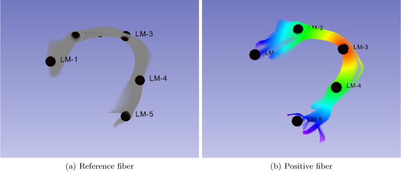
Example of landmarks for the Arcuate Fasciculus Right. 1(a) reference fiber bundle with landmarks. 1(b) distance color map of the third landmark, red means values closer to 0.

In a multi-class classification scenario, we aim to create 53 different classes. Since the number of classes is 53, this will increase the number of features to 268 and rend the neural network training impractical. To reduce the number of landmarks, we applied affinity propagation, which is a type of clustering algorithm that finds N “exemplars points” representative of a cluster given the number N. Figure 2 shows the number of landmarks kept after the affinity propagation algorithm was applied to the set of 265 landmarks (5 for each bundle) which is set to N = 32.

Figure 2.

Different views of the reference brain and associated reference landmarks represented by black points for the Multi-Classification case.

The computed landmarks in the reference atlas are propagated to a new subject via image registration using the fractional anisotropy images (FA) computed from the DTIs.

Once the landmarks are chosen, we compute the distance from every point in the fiber to each landmark plus the curvature and torsion at every point. The following section explains the design of the neural network.

3.2 Network model

Once the fibers have been processed and the features computed, we use this data as input to our network model as shown in Figure 4. The output of this network is a 2D matrix where the dimensions are the number of output classes n_class and the number of fiber tracts n_fib. The output of each fiber tract is a one-hot encoded vector, which means that it has the value 1 at the location of the predicted class and 0 everywhere else.

Figure 4.

Network model used during this study. Wi: Weight, Bi: bias

Let O_i be the predicted output, and T_i the target or ground truth,

$$D\left(O,T\right)=-{\displaystyle \sum _i^n{T}_i\log \left(O_i\right)}$$ (1)

this cross entropy or loss function measures the error between the predicted vector and ground truth vector.

The optimization will minimize the loss function using a gradient descent algorithm. During the optimization, the weights and biases at each layer are updated using back-propagation.

$$W=W_{\mathit{initial}}-\mu \frac{dL}{dW}B=B_{\mathit{initial}}-\mu \frac{dL}{dB}$$ (2)

μ is the learning rate set to 1⁻⁴, making sure the training does not diverge or over fit to the data. The number of epochs is set to 10. We used rectified linear units (ReLU) to break linearity in our network and speed up training. The following sections shows the results of our trained network.

4. RESULTS

The Arcuate Fasciculus Right Frontotemporal (ArcRFT) shown in Figure 5, was chosen to test our method because it is a bundle that is difficult to trace, is not always present, or it may be a short bundle.⁹ The role of this fiber bundle is still uncertain and current evidence suggests that it has an important role in language development.¹⁰ We used 8 different brain atlases of neonate infants of 1–2 years old to build our data set as follows.

• Training Set: 403676 negative single fibers + 13832 positive single fibers

• Validation Set: 44852 negative single fibers + 1536 positive single fibers

• n_pt: 50

• n_feat: 7 (5 landmarks + curvature + torsion)

Figure 5.

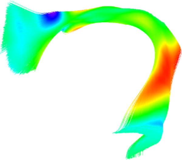
Arcuate Fasciculus Right Frontotemporal. Displayed using tensors coloring.

During training, the number of negative and positive samples were balanced. A batch of data is created by sampling the same numbers of fibers from the positive and negative set. During the optimization, each batch is generated randomly.

A binary/multi-class classification experiments were made. Our validation accuracy for the classification was ∼ 98.8%.

4.1 Binary classification

Figure 6 shows the results of the fiber tracing and classification using three different approaches. The automatically traced and classified fibers produced acceptable results as all fibers extracted correspond to the ArcRFT. Figures 7(a)–7(b)–7(c) show the classified fibers for the ArcRFT in different subjects. These figures appear to contain fibers that were miss-classified. However, after careful examination by our expert reviewer, these fibers do belong to ArcRFT. We highlight these results as they suggest that using purely geometric features, favors training our classifier. This is shown by the accuracy obtained in our test data set.

Figure 6.

Three results of ArcRFT from the same brain using different methods. The cleaning procedure proposed in Autotract is too aggressive and removes fibers that belong to the structure of interest.

Figure 7.

Other results of ArcRFT from different brains extracted using TRAFIC.

We tried our tool on fifty different brains of 1–2 years old. Our targets were the arcuate fasciculus fronto-temporal right and left. We classified the results in four categories: good, acceptable, empty, fail. As shown in Figure 8. A good or acceptable classification means a bundle was obtained with the proper characteristics of the ArcRFT or ArcLFT; empty classification means there were no fibers produced as output; a failed classification means the fibers were wrongly classified. For the ArcLFT, we obtained 70% of success, it is an acceptable result knowing that this bundle is difficult to trace. For the ArcRFT at least 52% of success and we note a big percentage of empty results (44%). It is known that the right fronto-temporal arcuate is absent in 40% females and 85% males.⁹ Additional validation is needed to verify the classifier is producing the right results and is not rejecting correctly traced fibers (false negative error). The failure rate is small for the ArcRFT (4%) compared to the ArcLFT(14%). This result indicates that the classifier is particularly strict concerning the ArcRFT, which could also explain the number of empty results. It is desired to have a strict classifier that rejects good fibers, than a classifier that accepts wrong fibers. We want to be sure than the label assigned to a fiber is correct. Those two requisites fit the description of a robust classifier and give us encouraging results to continue this research.

Figure 8.

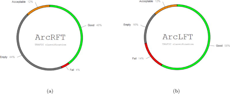
Classification results on 50 different arcuate fasciculus frontoTemporal right and left, ArcRFT and ArcLFT correspondingly.

4.2 Multi-class classification

The greatest challenge for this experiment was to prepare the training data set, i.e., it required cleaning fiber bundles for the classes used. Moreover, to obtain our rejection class, we needed to review the cleaning process in order to avoid including positive samples in the rejection class. For now, we have 3 different neonate infant brains of 1–2 years old as our data set. We recognize that our training data has a limited number of samples and we must do a cautious analysis of the results. The features used here include curvature, torsion and the euclidean distances to the 32 landmarks shown in Figure 2.

The focus of this experiment is the whole Arcuate Right, as shown in Figure 9(a), it is formed by three bundles: Arcuate Fasciculus Right Temporoparietal (ArcRTP), the Arcuate Fasciculus Right Frontotemporal (ArcRFT), the Arcuate Fasciculus Right Frontoparietal (ArcRFP).

Figure 9.

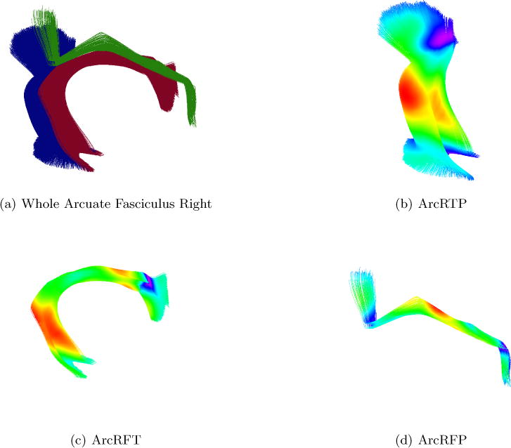
Arcuate Fasciculus Right and its three parts.

Visual assessment was done comparing TRAFIC with manually traced fibers as shown in Figure 10. Our results include fibers that do not belong to the bundle as shown in Figure 10(b) and 10(d). Nonetheless, they have similarities to the manually traced and the shape is preserved.

Figure 10.

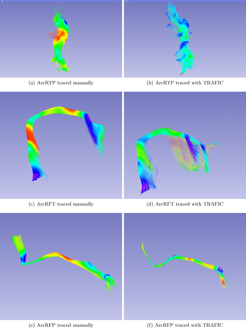
Two results of Arcuate Fasciculus Right from the same brain.

Further analysis is required but we assume that the source of miss-classification is our limited training data set and we predict that by increasing the number of samples, the classification power will improve. Nevertheless, the results presented in this paper are encouraging. TRAFIC classification requires 10 minutes to process a whole brain vs. Autotract which requires 3–4 hours to complete. This is a significant increase in efficiency.

5. CONCLUSIONS

We presented TRAFIC, a fully automated tool for the labeling and classification of brain fiber tracts. We demonstrated the utility of the proposed approach. The main advantages are its speed and accuracy for a fully automated method. As shown by the results, the binary and multi-class classification needs improvement. However, we predict that by increasing the number of training samples, the classification accuracy will increase. Different network architectures and Long-Short Term Memory (LSTM) networks that are useful for sequential data may also contribute to improve our classification power and will be used in future experiments.

Future work will be focused on creating 53 different classes of fiber bundles plus one rejection class in order to have a classifier for the most common traced bundles in the brain. TRAFIC will be included in the UNC-NAMIC framework and will provide automated classification for tractography methods.

Figure 3.

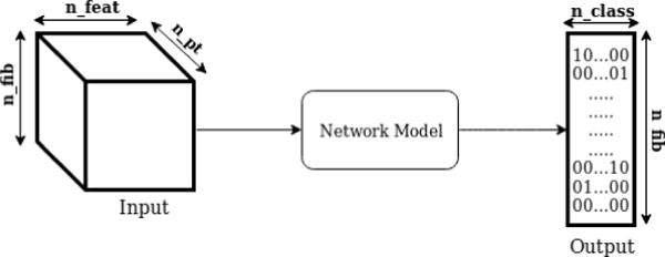
Global diagram. n_feat: number of features, n_pt: number of points, n_fib: number of fibers, nclass: number of output classes

References

- 1.Johansen-Berg Heidi, Behrens Timothy EJ. Diffusion MRI: from quantitative measurement to in vivo neuroanatomy. Academic Press; 2013. [Google Scholar]
- 2.Mori Susumu. Introduction to diffusion tensor imaging. Elsevier; 2007. [Google Scholar]
- 3.Prieto Juan C, Yang Jean Y, Budin François, Styner Martin. Autotract: Automatic cleaning and tracking of fibers. Proceedings of SPIE–the International Society for Optical Engineering. 2016;9784 doi: 10.1117/12.2217293. NIH Public Access. [DOI] [PMC free article] [PubMed] [Google Scholar]
- 4.Verde Audrey Rose, Budin Francois, Berger Jean-Baptiste, Gupta Aditya, Farzinfar Mahshid, Kaiser Adrien, Ahn Mihye, Johnson Hans J, Matsui Joy, Hazlett Heather C, et al. Unc-utah na-mic framework for dti fiber tract analysis. Frontiers in neuroinformatics. 2014;7:51. doi: 10.3389/fninf.2013.00051. [DOI] [PMC free article] [PubMed] [Google Scholar]
- 5.Oguz Ipek, Farzinfar Mahshid, Matsui Joy, Budin Francois, Liu Zhexing, Gerig Guido, Johnson Hans J, Styner Martin. Dtiprep: quality control of diffusion-weighted images. Frontiers in neuroinformatics. 2014;8 doi: 10.3389/fninf.2014.00004. [DOI] [PMC free article] [PubMed] [Google Scholar]
- 6.Goodlett Casey B, Fletcher P Thomas, Gilmore John H, Gerig Guido. Group analysis of dti fiber tract statistics with application to neurodevelopment. Neuroimage. 2009;45(1):S133–S142. doi: 10.1016/j.neuroimage.2008.10.060. [DOI] [PMC free article] [PubMed] [Google Scholar]
- 7.Joshi Sarang, Davis Brad, Jomier Matthieu, Gerig Guido. Unbiased diffeomorphic atlas construction for computational anatomy. NeuroImage. 2004;23:S151–S160. doi: 10.1016/j.neuroimage.2004.07.068. [DOI] [PubMed] [Google Scholar]
- 8.Fletcher P Thomas, Joshi Sarang. Riemannian geometry for the statistical analysis of diffusion tensor data. Signal Processing. 2007;87(2):250–262. [Google Scholar]
- 9.Marco Cantani and Marsel Mesulam. The arcuate fasciculus and the disconnection theme in language and aphasia: History and current state. Cortex. 2008;44:953–961. doi: 10.1016/j.cortex.2008.04.002. [DOI] [PMC free article] [PubMed] [Google Scholar]
- 10.Allendorfer Jane B, Hernando Kathleen A, Hossain Shyla, Nenert Rodolphe, Holland Scott K, Szaflarski Jerzy P. Arcuate fasciculus asymmetry has a hand in language function but not handedness. Human brain mapping. 2016;37(9):3297–3309. doi: 10.1002/hbm.23241. [DOI] [PMC free article] [PubMed] [Google Scholar]
Associated Data
This section collects any data citations, data availability statements, or supplementary materials included in this article.