Contribution of chromosomal polymorphisms to the G-matrix of Mimulus guttatus

Summary

• Evolution of genetic (co)variances (the G-matrix) fundamentally influences multitrait divergence. Here, we isolated the contribution of two chromosomal quantitative trait loci (QTLs), a meiotic drive locus and a polymorphic inversion, to the overall G-matrix for a suite of floral, phenological and male fitness traits in a population of Mimulus guttatus. This allowed us to predict the evolution of trait means and genetic (co)variances as a function of allele frequencies, and to evaluate theories about the maintenance of genetic variation in fitness.

• Individuals generated using a replicated F₂ breeding design were grown under common conditions, genotyped and measured for trait values.

• Significant additive genetic variance existed for all traits, and most genetic covariances were significantly nonzero. Both QTLs contribute to the additive genetic (co)variances of multiple traits. Pleiotropy was not generally consistent, either between QTLs or with the genetic background.

• Shifts in allele frequencies at either QTL are predicted to result in substantial changes in the G-matrix. Both QTLs contribute substantially to the genetic variation in pollen viability. The Drive QTL, and perhaps also the inversion, demonstrates the contribution of balancing selection to the maintenance of genetic variation in fitness.

Introduction

Understanding the processes that lead to phenotypic divergence is a central goal of evolutionary biology. Quantitative genetics has contributed greatly to this endeavor, in part because of the explicit recognition that phenotypic evolution results from both direct selection on a trait and indirect selection on genetically correlated traits (Lande, 1979; Arnold, 1994). The cornerstone of this approach is the genetic (co)variance matrix, or G-matrix, which describes the pattern of genetic variation and covariation among traits and thus determines the multivariate response to selection. Stability of the G-matrix is often assumed both for predicting long-term evolution and for retrospective analyses of past selection, an assumption that remains contentious (Turelli, 1988a; Phillips & Arnold, 1999; Roff, 2000; Steppan et al., 2002). Allele frequency changes at loci of major effect, particularly those that exhibit substantial pleiotropy, change the shape of the G-matrix and can significantly alter the rate and trajectory of multivariate evolution even in the short term (Turelli, 1988b; Carriére & Roff, 1995; Agrawal et al., 2001).

Mapping of quantitative trait loci (QTLs) is commonly used to investigate the genetic architecture of variation in traits (Tanksley, 1993). However, most QTL mapping studies focus on the genetics of differences between divergent populations or species, rather than on individual differences within populations. Even when crosses are conducted within populations, typical experiments evaluate marker-trait associations in progeny derived from a small number of parental genotypes (typically two), and thus are mute on the crucial detail of allele frequencies at QTL. In this study, we combined G-matrix and QTL approaches by employing a breeding design that incorporated 138 genomes randomly derived (Fig. 1) from a single natural population of Mimulus guttatus (Iron Mountain) located in central Oregon, USA. Using the replicated F₂ breeding design (Kelly, 2009), we estimated the overall G-matrix, as well as the contribution of two previously mapped QTLs to this matrix, for a suite of floral, phenological, and male fitness traits. This merger of QTL and G-matrix methods yields statistics that are quantitatively informative about the evolutionary potential of the Iron Mountain population for this collection of traits.

Fig. 1.

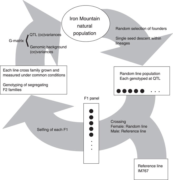
The overall plan for the experiment is depicted: field sampling followed by line extraction and experimental crosses, and finally estimation of genetic parameters specific to the natural population.

The floral traits examined were corolla size and shape and the relative lengths of anther and pistil. These characters affect mating system (Lin & Ritland, 1997; van Kleunen & Ritland, 2004; Fishman & Willis, 2008) and are under strong selection in the field (Fenster & Ritland, 1994; Willis, 1996). Our male fitness traits, the number of pollen grains per flower and the proportion of grains that are viable, covary with mating system (Ritland & Ritland, 1989; Fenster & Carr, 1997). They are also critical components of inbreeding depression (Carr & Dudash, 1997; Kelly, 2003) and post-zygotic reproductive isolation within the M. guttatus species complex (Fishman & Willis, 2001). Rate of development, measured as the number of days to reach bud and subsequent anthesis of the first flower (phenology), is a key component of local adaptation (Hall & Willis, 2006). Alterations in developmental timing of floral parts may represent key innovations in the radiation of Mimulus (Fenster et al., 1995). All of these traits are variable at multiple taxonomic levels within the M. guttatus species complex: between individuals within local populations, between local populations within species and between species. Differences are not limited to mean trait values: variances and covariances also differ among populations. Quantitative trait locus (co)variance estimates are particularly relevant for understanding the latter (Kelly, 2009).

Both QTLs that we investigate are chromosomal features for which the alternative ‘alleles’ can be directly scored by genotyping individuals at diagnostic molecular markers. The female meiotic-drive locus (alternative alleles D/d) is a chromosomal structural variant that appears to include the centromere of Linkage Group 11 (Fishman & Saunders, 2008); Mimulus chromosomes are identified according to the linkage maps of QTL studies, such as those of Fishman et al. (2002) and Hall et al. (2006). This locus was discovered because of extreme nonmendelian segregation in hybrids between an inbred line of Mimulus guttatus and its close relative Mimulus nasutus (Fishman et al., 2002; Fishman & Willis, 2005), but has subsequently been found to be polymorphic within the Iron Mountain M. guttatus population. In that population the region containing the drive locus exhibits extensive linkage disequilibrium, with the derived drive region consisting of a unique multilocus haplotype. The intraspecific segregation advantage of the D allele is more modest than in interspecific crosses but should have swept to fixation in the absence of a fitness cost. Fishman & Saunders (2008) have recently shown that the DD genotype suffers reduced pollen viability relative to D/d and d/d.

The second QTL is a polymorphic inversion on Linkage Group 6 (Lee, 2009). The Inversion polymorphism (alternative alleles C/c) was identified in a QTL mapping study of the Iron Mountain population. In that study, we synthesized three different F₂ mapping populations by crossing large-flowered to small-flowered genotypes. The linkage maps from each cross exhibited suppressed recombination among a large number of markers on Linkage Group 6. Subsequent genetic studies revealed extensive linkage disequilibrium in this genomic region within the Iron Mountain population (Lee, 2009). Specifically, the derived inverted segment (allele C) harbored a specific constellation of alleles at polymorphic marker loci on Linkage Group 6. Genotyping of these markers was used to identify Inversion type (i.e. QTL genotype) in this study. Reduced pollen viability consistently maps to this region and is associated with the C allele. Floral traits are also affected by this QTL, but the estimated effects are heterogeneous among different crosses.

Because these two QTLs have alleles readily identifiable by diagnostic marker alleles, we are able to estimate both allele frequencies and effects. Together, these determine the population-level genetic (co)variance contributed by each QTL (Kelly, 2009). We evaluate the percentage of the overall (co)variance explained by each QTL and assess consistency in pleiotropy across both QTLs as well as with the genetic background. This fulfills two distinct but complementary aims. First, we predict evolution of trait means, genetic variances and covariances as a function of allele frequencies at these two QTLs. Second, we use our results to evaluate theories about the evolutionary maintenance of genetic variation in fitness.

Materials and Methods

Estimating genetic parameters from the replicated F₂ design

The replicated F₂ design is a large collection of crosses between randomly extracted inbred lines and a common reference line drawn from the same population (Fig. 1). Each such ‘Line Cross Family’ consists of replicate individuals of the parental lines (denoted P_x for family x), F₁s and F₂s. Each random line is assumed to be fully homozygous and ‘random extraction’ implies that lines are representative of the natural population in terms of allele frequency at QTLs. Because both random lines and the reference line are fully homozygous, all F₁s within a particular line cross family are genetically identical. The F₂ subfamily is internally heterogeneous owing to segregation of allelic differences between the random and reference lines. Individuals of each type in each line cross family are grown under common conditions, measured for trait values, and genotyped at QTLs. While the replicated F₂ design is founded by inbred lines, most of the genotypes measured in the study are not highly homozygous (over 75% of the plants in our study are F₁s or F₂s). It thus circumvents the ‘artificial genetic background’ criticism often leveled at QTL studies based on recombinant inbred lines (RILs) or near-isogenic lines (NILs).

The phenotype of a plant was modeled as the sum of statistically independent genetic and environmental contributions. We ignored epistasis and parsed the entire genotypic value into two components, the effect of the QTL and the effect of the remainder of the genome:

$$\mathit{z}=g^{\prime }+{\mathit{g}}^{\ast }+\mathit{e}$$ Eqn 1

(z is the vector of phenotypic values for an individual; g′ is the vector of QTL effects on each trait; g* is the vector of background genotypic values; and e is the vector of environmental deviations. g* and e are random vectors, each with a covariance matrix to be estimated from the data. These are the usual G-matrix and E-matrix of evolutionary quantitative genetics (Arnold, 1992), although the former is minus the contribution of the particular QTL(s) characterized by g′.

Our approach assumes that the entire collection of phenotypic measurements from the experiment follows a multivariate normal distribution. Based on this, we maximized the likelihood (probability density function) for the data (Shaw, 1987; Searle et al., 1992). With multinormality, the model is fully articulated if the expected values and (co)variances of measurements are expressed as a function of model parameters, either fixed effects or variance components. The former determine the expected value of measurements and the latter determine the covariance of residuals from these expectations. Because our two QTL are ‘Known Alleles QTL’ in the terminology of Kelly (2009), g′ are estimated as fixed effects. We let a denote the additive effect of the QTL allele that is homozygous in the reference line and d denote the dominance effect (genotypic parameterization of Falconer & Mackay, 1996, ch. 7).

The expectations and covariances for g* with additive genetic effects at background loci are given in Appendix 1 of Kelly (2009). However, previous studies of Iron Mountain M. guttatus indicate that quantitative traits typically exhibit directional dominance or inbreeding depression (Willis, 1996; Kelly & Arathi, 2003). A generalization of the replicated F₂ design equations for a single trait with an arbitrary number of loci, arbitrary numbers of alleles per locus and arbitrary dominance is given in the Supporting Information, Notes S1. These equations retrieve the additive model as a special case. With dominance, it is necessary to estimate distinct means for the reference line (P₀), the population of random lines (P_x), and the population of F₁ plants. However, the F₂ mean is then constrained:

$$E[{\overline{z}}_{{\mathrm{F}}_2}]=(2E[{\overline{z}}_{{\mathrm{F}}_1}]+E[{\overline{z}}_{{\mathrm{P}}_0}]+E[{\overline{z}}_{{\mathrm{P}}_x}])/4$$ Eqn 2

( ${\overline{z}}_{\ast }$ denotes the observed mean of a group and E[*] is the expectation).

Species and experimental protocols

Mimulus guttatus DC (2n = 28) is a small, self-compatible wildflower that occurs throughout western North America. Local populations may be either annual or perennial and there is extensive variation in mating system. The plants of this study are derived from Iron Mountain, which is a large, annual (or winter annual) population located in the Cascade Mountains of central Oregon (Willis, 1996). This population is predominantly outcrossing (Willis, 1993).

J. H. Willis randomly sampled line founders from Iron Mountain in August of 1995 (Willis, 1999). Each line was subsequently propagated by single-seed descent with conscious effort to avoid selection. These lines are now 8–14 generations inbred and have been confirmed to be homozygous at highly polymorphic microsatellite markers (Kelly, 2003). We chose a specific inbred line, IM767, from Iron Mountain to use as our reference line. This line was used as a pollen donor to produce F₁ hybrids with each of 138 of the random lines. A single F1 plant from each cross was subsequently self-pollinated to produce an F₂ family.

From each line cross family, we attempted to grow and measure 12 F₂ progeny, six F₁ progeny, and six individuals of the random parental line. We also grew and measured 339 individuals from IM767, the reference line. Owing to germination failure or failure to flower, the actual size of each line cross family was often less than the full complement of 24 plants. After eliminating a small fraction of plants owing to ambiguities in genotyping (see below), the final sample size was 3118 plants. Germination was staggered across four ‘cohorts’, each separated by 1–2 wk. Each line cross family spanned two cohorts and the reference line was grown in each cohort. Plants were grown in a glasshouse with light augmentation (18 h daylength). Beginning 14 d after sowing, plants were fertilized every week using N–P–K (10 : 30 : 20) at a concentration of 3.95 g l⁻¹ of water. Plants began flowering 19 d after sowing.

For most plants in the study, we were able to note the day on which the first flower bud erupted from the meristem. Bud duration is the time from this event until anthesis of the first flower. Four morphological measurements were taken on the days in which each plant produced its first and second flowers: corolla width, corolla length, pistil length, and anther length. Stigma–anther separation is calculated as the difference between the last two measurements. We collected pollen from the first two flowers and stored it in microcentrifuge tubes for later counting. The total number of viable and nonviable pollen grains per flower was estimated using a Coulter Counter Model Z1 (Coulter, Miami, FL, USA) dual (for detailed description of these procedures see Kelly et al., 2002; Kelly, 2003).

Alternative alleles of the drive locus can be identified cytogenetically (Fishman & Saunders, 2008), but it is more efficient to genotype diagnostic marker loci. We used a length polymorphic marker HB5 as an indicator of genotype at the Drive QTL. HB5 allele length 277 (bp) was classified as D while all other allele lengths were classified as d. The derived Inversion QTL allele, C, was identified by a specific combination of alleles at two different marker loci: allele length 240 at marker locus MgSTS431 and allele 201 at MgSTS229. All other allelic combinations were assigned c. The QTL genotype assignments from marker data were based on genetic analyses subsequent to QTL screens (Y. W. Lee & L. Fishman, unpublished). Any error caused by these assignments, or recombination between marker and QTL, will reduce the estimated effects of the QTLs, thus making our tests conservative. IM767 is homozygous for the ancestral allele at both QTLs (c and d).

DNA extraction and genotyping were done in a 96-well format. Young leaves were collected from each measured F₂ plant and from a single F₁ and parental plant of each line cross family. We extracted DNA using our standard laboratory pipeline (Marriage et al., 2009) and amplified marker loci using a touchdown PCR protocol (Hall & Willis, 2005). All markers were length polymorphic and PCR-amplified fragments were detected on an ABI 3130 genetic analyser (Applied Biosystems). We scored size fragments using the genemapper 4.0 software (Applied Biosystems). We first genotyped the parental lines and F₁s from each line cross family to determine the families that were segregating for each QTL. We then genotyped F₂ progeny of polymorphic families. Measurements were eliminated if there was any inconsistency between parental and progeny genotypes.

Model fitting and evaluation procedures

We first fitted the general linear model (GLM) to each trait individually using maximum likelihood. We let Yijklmn denote the trait value(s) of the nth individual of type i (reference line, random line, F₁ or F₂) in family m, cohort j, with Drive QTL genotype k and Inversion QTL genotype l:

$$Y_{\text{ijklmn}}={\mathrm{\mu }}_{\mathrm{i}}+{\mathrm{\gamma }}_{\mathrm{j}}+g_{\mathrm{k}}^1+g_{\mathrm{l}}^2+g_{\text{ijklmn}}^{\ast }+e_{\text{ijklmn}}$$ Eqn 3

(μ is the mean of type i; γ is the (fixed) effect of cohort (j = 1, 2, 3, 4); g¹ is the (fixed) effect of the genotype at the drive locus; g² is the (fixed) effect of the genotype at the inversion locus; $g_{\text{ijklmn}}^{\ast }$ is the (random) effect of the genomic background; $e_{\text{ijklmn}}^{\ast }$ is the (random) environmental deviation for individual n). Both $g_{\text{ijklmn}}^{\ast }$ and $e_{\text{ijklmn}}^{\ast }$ are independent of the fixed effects and each other. When fitting the model to pairs of traits, each trait has a distinct set of effects. This is a mixed model and the full log-likelihood for the dataset, l, has a closed form (Shaw, 1987; Searle et al., 1992, p. 234).

The most general model, allowing arbitrary dominance at loci contributing to the genetic background and effects from both QTLs, has 15 parameters: 10 fixed effects (means for the reference line, random lines and F₁s, the three cohort effects and the additive (a) and dominance (d) effect of the reference line allele for each QTL) and five variance components (V_E, C₁₁, C₁₂, C₂₂ and V_S). We determined the log-likelihood of this most general model and compared it with more restricted models using both likelihood ratio tests and AIC (Akaike information criterion) (Burnham & Anderson, 2002). Two sorts of restriction were considered: we can reduce the complexity of the genetic background model by assuming additivity, resulting in either two or three variance components, and one fewer fixed effect (see Notes S2); we can also eliminate one or both of the QTLs, deleting two or four fixed effects from the parameter set.

After analysing the single trait results, we adopted the fully general model for fixed effects (Eqn 2) and the intermediate complexity three-parameter additive model for estimating the genetic covariances between traits (see Notes S2). Under this assumption, the single trait variance components are the additive variance of the genetic background (denoted V*_A[x] for trait x), the environmental variance (V_E[x]) and the segregational variance (V_S[x]). The segregational variance is determined by gametic variation specific to the reference line (Kelly, 2009). If many additive loci contribute to the genetic background, then V_S[x] should be approximately equal to $V_{\mathrm{A}[\mathrm{x}]}^{\ast }/4$. For two traits (x and y), the corresponding covariances are $C_{\mathrm{A}[\text{x,y}]}^{\ast }$, C_E[x,y] and C_S[x,y]. In applying Eqn 3 to a trait pair (x and y), we estimate 29 parameters: the 13 parameters for each trait, plus $C_{\mathrm{A}[\text{x,y}]}^{\ast }$, C_E[x,y] and C_S[x,y].

To maximize the log-likelihoods for all models, we used a combination of stochastic hill-climbing and Markov Chain Monte Carlo (MCMC) search executed in a matlab program (code written by A.G.S. available upon request). An initial stochastic search, in which steps are only taken if they increase the log-likelihood, was run until the log-likelihood improved by less than 0.001 per thousand iterations. In each iteration, a new set of parameter values was obtained by adding a vector of normal deviates with variance δ and mean 0 to the current vector. The magnitude of δ was adjusted periodically to maintain an intermediate step frequency.

Following the initial search, we conducted at least six cycles of MCMC followed by stochastic search. The MCMC search proceeded in the same way as the stochastic search, except that downhill steps were taken with probability equal to the ratio of the new (suggested) and current likelihoods (Metropolis et al., 1953). Each cycle involved 500 iterations of MCMC, followed by uphill stochastic search starting from the endpoint of the MCMC. The stochastic search continued until convergence. The parameter set that yielded the highest log likelihood over the course of the entire search was retained. To ensure validity of the algorithms, we wrote a parallel set of programs in C (code by J.K.K. available upon request). All results are fully congruent between these two different platforms.

Results

The means and standard deviations of measurements for each type of plant in our breeding design are given in Table 1. The floral traits and pollen counts are averages of measurements from the first two flowers, except where measurements were missing. The phenological traits apply to the first flower only. The morphological traits and bud duration each exhibited a roughly normal distribution of values (within types) and were analysed on their original scale of measurement. Stigma–anther separation was calculated from the difference between stigma and anther lengths and thus is not an independent trait. ‘Days to bud’ was right-skewed, which we addressed by applying a square-root transformation. We also log-transformed total pollen and applied the angular transformation (arcsin square-root) to the proportion of grains viable. The transformed values were used in QTL and G-matrix estimation (all figures).

Table 1.

The means and SD are given for each trait, before and after transformation, for each type of Mimulus guttatus plant

Trait	Statistic	IM767	Random lines	F1 plants	F2 plants
Corolla width (CorWid)	Mean	18.80	16.63	19.32	18.53
	SD	2.09	2.89	2.76	2.82
Corolla length (CorLen)	Mean	21.05	20.42	22.53	21.72
	SD	1.91	2.85	2.59	2.71
Anther length (Anther)	Mean	12.13	11.22	12.44	12.01
	SD	0.77	1.29	1.03	1.19
Pistil length (Pistil)	Mean	14.26	13.68	14.58	14.28
	SD	0.94	1.64	1.22	1.37
Stigma-anther separation (SA)	Mean	2.15	2.48	2.15	2.27
	SD	0.57	1.07	0.69	0.90
Pollen viability	Mean	0.81	0.60	0.82	0.76
	SD	0.13	0.18	0.12	0.15
ArcSin Sqrt pollen viability (PV)	Mean	1.14	0.89	1.15	1.08
	SD	0.15	0.19	0.16	0.18
Total pollen	Mean	10 340	5194	11 449	9641
	SD	3544	2988	3887	3934
Log total pollen (Pollen)	Mean	3.99	3.65	4.03	3.94
	SD	0.17	0.25	0.17	0.21
Days to bud	Mean	21.59	22.85	19.71	20.72
	SD	5.78	4.73	4.45	3.96
Sqrt Days to bud (DTB)	Mean	4.61	4.76	4.41	4.53
	SD	0.60	0.48	0.47	0.42
Bud duration (Bud)	Mean	8.55	7.92	7.91	7.95
	SD	1.10	1.39	1.20	1.20

The abbreviations used subsequently are given in parentheses. Sqrt indicates the SquareRoot transformation.

Genotyping of the 138 random lines showed that 55 were DD while only four were CC. Thus, allele frequencies for the derived QTL alleles within the parental lines were p(D) = 0.41 (p(d) = 0.59) and p(C) = 0.03 (p(c) = 0.97), respectively. At the drive locus, a total of 574 F₂ individuals were successfully genotyped and 145 were DD, 285 were Dd, and 144 were dd. Interestingly, this marker showed no segregation distortion. The inversion appeared to segregate normally in the four polymorphic line cross families, but samples sizes were not sufficient for a meaningful test for segregation distortion.

The single trait analyses involved 144 model fits: 16 models for each of nine traits (Notes S2). Comparisons of maximum likelihood values indicated that (1) dominance significantly alters both the fixed effects and variance components of the genetic background model, and (2) the estimated contribution of QTLs to trait variation and the statistical significance of these effects are relatively independent of the genetic background model. Regarding (1), constraining the means of F₁ and F₂ families to the midpoint of the reference line and mean of random lines (as expected with additive gene effects) greatly reduced likelihoods (i.e. elevates AIC values, Table S2). In other words, all traits exhibited significant directional dominance (inbreeding depression). Even after accommodating dominance for fixed effects, we found that the dominance model for variance components (five parameters) is favored over the additive model (three or two parameters) for eight of the nine traits (Table S2).

Importantly, QTL effect estimates are relatively independent of the genetic background model. We compared maximum likelihoods from four QTL models: no QTLs, the Drive QTL only, the Inversion QTL only and both QTLs included. Excluding the additive fixed effect model (the background model that yields uniformly low likelihoods), the same QTL model is invariability selected for a particular trait regardless of the model for the genetic background (bold type in Table S2). Table 2 reports QTL effect estimates using the three-parameter additive model for the genetic background. This model was chosen for entirely practical reasons. Additive (co)variances cannot be disentangled from nonadditive components with the more general background model in the replicated F₂ design (see Notes S1). To extract parameter estimates that are directly comparable to those obtained in other G-matrix studies, we also used the three-parameter additive model for estimating genetic covariances among traits.

Table 2.

Results of model fitting are described for single trait data from Mimulus guttatus

	Drive QTL		Inversion QTL
Trait	a	d	a	d
CorWid	−0.015 (0.05)	−0.008 (0.05)	0.205 (0.17)	0.230 (0.15)
CorLen	0.019 (0.05)	−0.067 (0.06)	0.015 (0.17)	0.084 (0.16)
Anther	0.028 (0.05)	−0.018 (0.06)	0.169 (0.18)	0.155 (0.16)
Pistil	−0.080 (0.05)	−0.063 (0.05)	0.318 (0.18)	0.147 (0.15)
SA	−0.170 (0.05)	−0.073 (0.05)	0.241 (0.18)	0.057 (0.15)
PV	0.225 (0.04)	−0.067 (0.06)	0.609 (0.15)	−0.218 (0.16)
Pollen	0.099 (0.04)	0.076 (0.06)	0.324 (0.14)	−0.165 (0.17)
DTB	0.034 (0.05)	0.172 (0.07)	0.294 (0.14)	0.492 (0.19)
Bud	−0.031 (0.04)	0.018 (0.07)	−0.329 (0.12)	−0.161 (0.20)

Allelic effects, a and d, are attributed to the ancestral allele and are in units of phenotypic SD. Standard errors, determined from the asymptotic dispersion matrix of the likelihood model, are given in parentheses. Bold type indicates the QTL has a significant effect on the trait.

CorWid, corolla width; CorLen, corolla length; Anther, anther length; Pistil, pistil length; SA, stigma-anther separation; PV, arcsin squareroot (sqrt) pollen viability; Pollen, log total pollen; DTB, sqrt Days to bud; Bud, bud duration.

Neither QTL had significant effects on the corolla width, corolla length, or anther length. Pollen viability, total pollen, and days to bud were affected by both QTL. Stigma–anther separation was affected by the Drive QTL, while pistil length and bud duration were affected by the Inversion QTL (Table 2). The ancestral alleles for both QTL have positive additive effects on the pollen traits and on days to bud. The d allele reduced stigma–anther separation while the c allele reduced bud duration. Genetic dominance is evident and variable within and between QTLs. Estimates suggested overdominance for both QTLs in their effects on days to bud.

The pattern of QTL significance for effects on pistil length, anther length and stigma–anther separation merits comment. The ancestral drive allele significantly reduces stigma–anther separation mainly by reducing pistil length. The former effect is significant while the latter is not. This is likely because the strong positive environmental covariance between pistil and anther lengths was ‘factored out’ of stigma–anther separation. Indeed, the heritability of the stigma–anther separation was substantially greater than for either component trait (Table 3a). The ancestral (noninverted) allele at the second QTL appeared to increase the lengths of both pistil and anthers, although only the larger effect on pistil length was significant. The estimated effect of the Inversion QTL on stigma–anther separation, while larger than for the Drive QTL, is not significant. This is unsurprising given that standard errors were generally much larger for Inversion QTL estimations owing to the fact that this QTL was segregating within only four line cross families.

Table 3.

Whole genome (a) and quantitative trait locus (QTL)-specific (b) additive (co)variances are given for Mimulus guttatus

	CorWid	CorLen	Anther	Pistil	SA	PV	Pollen	DTB	Bud
(a) Whole-genome additive (co)variances
CorWid	0.406	0.275	0.157	0.241	0.174	0.019	0.079	0.047	0.001
CorLen		0.354	0.255	0.283	0.122	0.003	0.057	0.054	−0.020
Anther			0.373	0.290	−0.025	0.000	0.073	0.036	−0.024
Pistil				0.422	0.294	0.051	0.110	0.030	−0.024
SA					0.479	0.076	0.082	0.005	−0.008
PV						0.236	0.097	0.029	−0.023
Pollen							0.155	0.016	−0.024
DTB								0.129	−0.055
Bud									0.060
(b) QTL-specific additive genetic (co)variances
CorWid	0.0000   0.0000	−0.0002	−0.0002	0.0005	0.0010	−0.0016	−0.0006	0.0000	0.0002
CorLen	0.0000	0.0005   0.0002	0.0005	−0.0010	−0.0024	0.0036	0.0013	0.0000	−0.0005
Anther	0.0000	−0.0001	0.0005   0.0000	−0.0010	−0.0024	0.0036	0.0013	0.0000	−0.0005
Pistil	−0.0001	−0.0007	0.0002	0.0023   0.0019	0.0052	−0.0078	−0.0028	−0.0001	0.0011
SA	−0.0001	−0.0007	0.0003	0.0020	0.0119   0.0020	−0.0180	−0.0065	−0.0002	0.0026
PV	−0.0005	−0.0030	0.0011	0.0085	0.0089	0.0272   0.0386	0.0098	0.0004	−0.0039
Pollen	−0.0003	−0.0018	0.0006	0.0050	0.0052	0.0227	0.0035   0.0134	0.0001	−0.0014
DTB	0.0001	0.0006	−0.0002	−0.0018	−0.0018	−0.0080	−0.0047	0.0000   0.0017	−0.0001
Bud	0.0001	0.0007	−0.0002	−0.0019	−0.0019	−0.0084	−0.0050	0.0017	0.0006   0.0018

All estimates are in standardized units (the phenotypic variance of each trait is 1) and significantly nonzero values are bold. (a) The additive genetic variances (equal to the narrow sense heritabilities) are on the diagonal and covariances are given above the diagonal. (b) QTL additive genetic variances are on the diagonal (drive above, inversion below). The QTL covariances are above the diagonal for the Drive QTL and below the diagonal for the Inversion QTL.

CorWid, corolla width; CorLen, corolla length; Anther, anther length; Pistil, pistil length; SA, stigma-anther separation; PV, arcsin squareroot (sqrt) pollen viability; Pollen, log total pollen; DTB, sqrt Days to bud; Bud, bud duration.

The overall G-matrix for these traits was estimated by considering all trait pairs without distinguishing QTLs (Table 3a). This is the (co)variance matrix for the aggregate quantity (g′ + g*) in Eqn 1. All traits exhibited significant additive genetic variation and most of the additive genetic covariances were significantly nonzero. Genetic (co)variances were classified as significantly nonzero based on the likelihood ratio test with 2 df – no genetic (co)variation reduces the model by two parameters (V_A[x] = V_S[x] = 0 or CA[x,y] = CS[x,y] = 0).

Combining QTL allelic effect estimates with the allele frequencies in our line sample yielded estimates for QTL (co)variances (Table 3a). With two alleles,

$$V_{\mathrm{q}[\mathrm{x}]}=2p(1-p){(a_{\mathrm{x}}+d_{\mathrm{x}}(1-2p))}^2$$ Eqn 4

is the QTL additive genetic variance for trait x. There is a nonzero QTL covariance for each trait pair that is jointly influenced by a single QTL.

$$C_{\mathrm{q}[\text{x,y}]}=2p(1-p)(a_{\mathrm{x}}+d_{\mathrm{x}}(1-2p))(a_{\mathrm{y}}+d_{\mathrm{y}}(1-2p))$$ Eqn 5

is the QTL additive covariance for traits x and y. In Eqns 4 and 5, the genotypic effects (a and d) are attributed to the allele with population frequency p (Falconer & Mackay, 1996, p. 126).

The estimated (co)variance attributable to the genetic background, g* of Eqn 1 or $g_{\text{ijklmn}}^{\ast }$ of Eqn 3, is the difference between corresponding terms in Table 3. The differences between QTL-specific (co)variances and trait associations generated by the remainder of the genome characterize variable pleiotropy from a population perspective. For example, the joint effects of the Drive QTL on pollen viability and stigma–anther separation are depicted in Fig. 2. The ellipses represent the joint distribution for genetic background values in the population. The major and minor axes of the ellipse were calculated from the background additive genetic (co)variances of these two traits. The major axis is the dimension of greatest genetic variability (Schluter, 1996) and its length is twice the corresponding standard deviation.

Fig. 2.

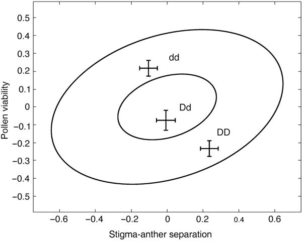
The drive quantitative trait locus (QTL) genotypic means in relation to the background genetic (co)variance between viable pollen per flower and stigma–anther separation in Mimulus guttatus. The bivariate means for each genotype (DD, Dd and dd) are given ± 1 SE relative to the overall population mean (centered at 0, 0). The length of the primary axis of the larger ellipse is equal to twice the square root of the largest eigenvalue of the background G-matrix.

Discussion

The G-matrix summarizes inheritance for multiple phenotypic traits and fundamentally influences the evolution of trait means in response to selection (Hazel, 1943; Lande, 1979). Correlated evolution of multiple traits is common, and patterns of trait association are often consistent across multiple levels of divergence (Gould, 1966; Harvey & Pagel, 1991). Theoretical considerations suggest that evolution proceeds most readily along the principle axis of the G-matrix, which is the multivariate direction of greatest additive genetic variance. Patterns of morphological divergence between species seem to be biased towards this ‘genetic line of least resistance’ (Schluter, 1996). Of course, quantitative prediction of diversification depends on the stability of, or predictability of changes in, the G-matrix through time. Understanding the rate and pattern of G-matrix evolution remains a central objective in evolutionary biology (Arnold et al., 2008).

A key issue for G-matrix evolution is the magnitude and diversity of phenotypic effects associated with individual QTLs. Genetic ‘step size’ has been discussed extensively in relation to diversification (Gottlieb, 1984; Coyne & Lande, 1985) and there is empirical evidence that genes of major effect contribute to adaptation (Orr & Coyne, 1992; Bradshaw et al., 1998). If diversification occurs through the recruitment of standing genetic variation, then the distribution of phenotypic effects across polymorphic loci should be a primary target for experimental studies. Robertson (1967) argued that this distribution of effects is likely to be exponential, with a few major QTL segregating along with a great many relatively minor loci. In the short term under directional selection, allele frequency changes at major QTL are likely to have the most pronounced effect on the G-matrix (Agrawal et al., 2001). However, initial allele frequency and pleiotropy are as important as effect size in identifying a QTL as major in this context (Kelly, 2009).

Our approach is based on the recognition that genetic (co)variances are aggregate functions of QTL allele frequencies and effects (Turelli, 1988b; Phillips & McGuigan, 2005) and that the genomic components of the G-matrix are estimable statistics (Kelly, 2009 and references therein). In this study, we estimate a G-matrix for floral and life history traits in the Iron Mountain population of Mimulus guttatus. The overall matrix (Table 3a) is subsequently decomposed into portions contributed by each of two specific QTLs (Table 3b) and a remainder from the rest of the genome. In the following sections, we first review our results in relation to the extensive quantitative genetic literature on M. guttatus and then discuss how QTL estimates can be translated into predictions for G-matrix evolution. We also consider the QTL (co)variance estimates in relation to evolutionary models for the maintenance of genetic variation. Finally, we review a series of important assumptions/caveats associated with these conclusions and with our approach in general.

The G-matrix for Mimulus guttatus at Iron Mountain

Our character set includes measures of flower size, the relative positions of reproductive structures, phenology, and male reproductive capacity (Table 1). All traits exhibit significant additive genetic variation. The narrow sense heritability is highest for floral morphology, intermediate for male fitness traits and lowest for the phenological traits (diagonal of Table 3a). Our estimates for morphology and male fitness traits are close to those obtained in previous studies of the Iron Mountain population (see Table 2 of Kelly & Arathi, 2003; Table 3 of Kelly, 2003), although present estimates are slightly higher because we averaged measurements from two flowers.

The strong positive genetic correlations between floral morphology with total pollen are unsurprising, but the significant relationship between pollen viability and corolla width is notable. Genetic correlations with the phenological traits were generally nonsignificant (except for corolla length with days to bud), but this is likely caused by a lack of power. Artificial selection on corolla size induces a correlated response in days to flower (Holeski & Kelly, 2006; Kelly, 2008). When QTLs are included in the model (Table 3b), genetic correlations involving the phenological traits are clearly identified. The Inversion QTL generates a negative covariance between bud duration and both pollen traits while the Drive QTL generates a negative covariance between stigma–anther separation and days to bud. These results indicate the increase in power achieved by including QTLs in breeding designs for G-matrix estimation.

When compared with previous studies, our results contribute to accumulating evidence that the G-matrix is quite malleable within the M. guttatus species complex. For the same collection of morphological characters, much lower (but still positive) V_A estimates have been obtained from a California population (Robertson et al., 1994) and a largely clonal population on the Oregon coast (T. Marriage, unpublished). By contrast, Carr & Fenster (1994) obtained V_A estimates generally greater than those in Table 2 from two other Californian populations of M. guttatus. Self-fertilizing populations/taxa within the complex have highly reduced flowers and the total phenotypic variances of flower size within such populations are typically less than V_A of outcrossing populations (see Table 2 of Carr & Fenster, 1994). With respect to covariances, van Kleunen & Ritland (2004) estimated a strongly negative genetic correlation between pollen viability and corolla width, while our estimate is significantly positive (Table 2). The observed differences in genetic (co)variation patterns among populations of the M. guttatus complex motivates a more fine-scale consideration of the genomic regions responsible for variation.

QTL (co)variances and multivariate evolution

The QTL (co)variances shed light on how the G-matrix is likely to evolve. Our experiment isolated the contribution of two chromosomal QTLs to the overall G-matrix. The Drive QTL (Linkage Group 11) and the Inversion QTL (Linkage Group 6) each affect pollen viability, total pollen and days to bud. Stigma–anther separation is significantly influenced by the Drive QTL, while bud duration is affected by the inversion (Table 3). Previous mapping studies had demonstrated the effect of these QTLs on pollen viability (Fishman et al., 2002; Fishman & Saunders, 2008; Lee, 2009), but the allele-specific effects on stigma–anther separation and on the developmental timing traits are novel to this experiment.

With estimates for allele frequencies, effect sizes, pleiotropy, and dominance, we can explore the role of these loci in creating, maintaining, or reducing genetic constraints. For example, the Drive QTL contributes a negative covariance between stigma–anther separation and pollen viability. This is directly opposite to the overall positive genetic covariance between these two traits (Fig. 2). As a consequence, changes in allele frequencies at this QTL will result in evolution along the line of greatest genetic resistance. Fixation of either QTL allele would reduce the genetic variances of these traits, but increase the magnitude of the genetic correlation.

Figures 3 and 4 explore the evolution of the overall G-matrix for trait pairs as a function of allele frequencies at one or both QTLs. Here, the major and minor axes of each ellipse are functions of the genetic (co)variances for these traits. At the endpoints in these figures, where QTL allele(s) are fixed, the ellipse represents the background genetic (co)variance. The background (co)variance is calculated by subtracting the QTL (co)variance (Table 3b) from the overall additive (co)variance (Table 3a). These figures provide an empirical example of trajectories predicted by Agrawal et al. (2001) for G-matrices with selection on major QTLs.

Fig. 3.

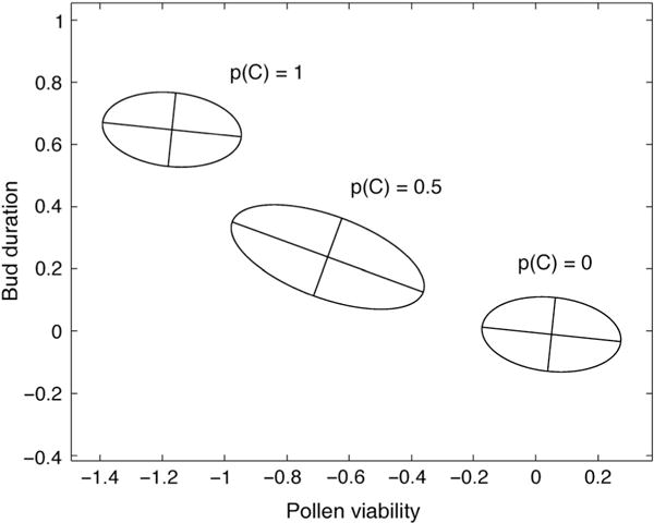
The joint distribution of additive genetic values for Mimulus guttatus bud duration and pollen viability is depicted for three different values for p(C), the frequency of the derived Inversion allele. The axes of each ellipse are calculated from the estimated G-matrix of these two traits at that value of p(C). Axis lengths are equal to the square root of their associated eigenvalues.

Fig. 4.

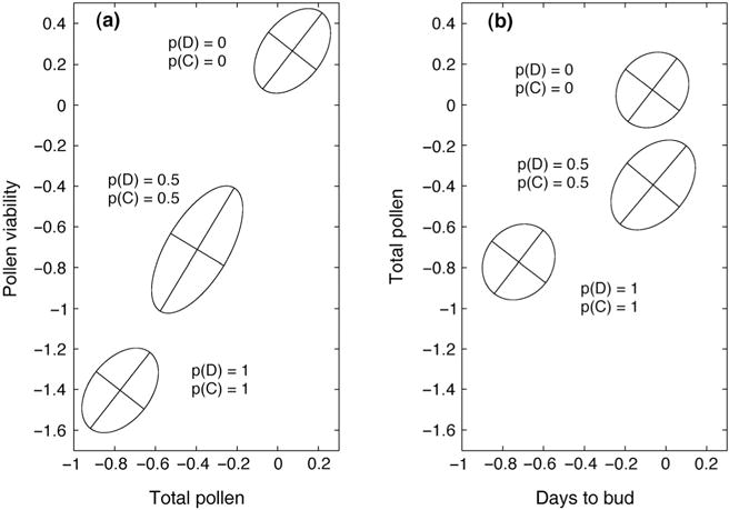
The joint distribution of additive genetic values is depicted in populations of Mimulus guttatus with both QTL fixed for the derived allele (p(C) = p(D) = 1), both QTL fixed for the ancestral allele (p(C) = p(D) = 0), and at intermediate allele frequencies (p(C) = p(D) = 0.5). The axes of each ellipse are calculated from the estimated G-matrix of these two traits at that value of p(C). Axis lengths are equal to the square root of their associated eigenvalues.

Figure 3 considers only the Inversion QTL, which creates a negative covariance between pollen viability and bud duration. Genotypic values for the Inversion QTL do not follow the classical expectation wherein heterozygotes have the lowest pollen viability owing to crossovers within the inversion that generate aneuploid gametes (Darlington, 1937; Sturtevant, 1938). Instead, heterozygotes have intermediate means for both traits. The Inversion QTL contributes fully one-third of the total negative genetic covariance between pollen viability and bud duration, even at the extreme allele frequency of our parental line population (p(C) = 0.03). If allele frequency is shifted to 0.5, the Inversion QTL would generate an estimated negative covariance that is 7.7 times that of the genomic background (central ellipse in Fig. 2). Evolution at this QTL would substantially alter both the eigenvalues and eigenvectors of the G-matrix (Phillips & Arnold, 1999).

Figure 4 considers simultaneous changes at both QTLs. In contrast to Fig. 2, the relationship between male fitness traits and days to bud is characterized by consistent pleiotropy. Both QTLs and the genetic background contribute positive covariance to pollen viability and total pollen. Changes in QTL allele frequency alter the magnitude but not the direction of the covariance (Fig. 4a). Allelic substitutions here would represent evolution along the path of least resistance. For days to bud, both QTLs display a pattern of overdominance. This causes the direction of their contribution to covariance to change with allele frequencies (Fig. 4b). When the derived alleles are frequent (high values for p(C) and p(D)), both QTL contribute positively to the genetic covariance of total pollen and days to bud. When C and D are rare, however, both QTLs contribute negatively to the covariance. Over-dominance also results in curvature of the evolutionary trajectory as allele frequencies change, even though trait means ultimately shift along the genetic line of least resistance (Fig. 4b). This curvature could not be predicted from the G-matrix without information about QTL-specific details.

The maintenance of genetic variation in male fitness

Our estimates for QTL effects and allele frequencies suggest that over one-fourth of the additive genetic variance in pollen viability is generated by the Drive and Inversion QTLs. These results are intriguing in light of previous quantitative genetic studies of pollen viability variation within Iron Mountain. Mutation-selection balance is a natural null model for a trait like pollen viability, which (all else being equal) should be under strong directional selection. We previously used a breeding design that involved both inbred and outbred plants to estimate the inbreeding load, the additive genetic variance and several inbreeding variance components for pollen traits (Kelly, 2003). These estimates indicated an excess of additive genetic variation relative to the expectation under mutation– selection balance and we rejected several explicit models in which variation is caused by rare, partially recessive alleles.

The chromosomal feature QTLs (Table 3) are concrete examples of the kind of loci that were predicted to exist, but not identified by the quantitative genetic study of Kelly (2003). The alternative alleles at the Drive QTL segregate at intermediate frequency and are likely maintained by a balance between individual and gametic selection (Fishman & Saunders, 2008). The derived Inversion type (allele C) is homozygous in only 3% of random lines and could be considered deleterious. However, allele C is likely more common in the wild population (see below), and given its pronounced effect on the phenotype, it would be surprising for an unconditionally deleterious mutation to reach even 3% in a large stable population such as that of Iron Mountain. With respect to our previous arguments based on variance components, it is important that the rare allele at the Inversion QTL is partially dominant with respect to its pollen effects (Table 2). Rare dominants make a much larger variance contribution than rare recessives and have a wholly different signature in a population’s response to inbreeding (Cockerham & Weir, 1984).

Caveats

The quantitative merger of QTL mapping with G-matrix estimation requires that the mapping population is genetically representative of the natural population (Kelly, 2009). Our parental lines were initiated from random field plants, but subsequently propagated by successive generations of self-fertilization (Fig. 1). Lethality and sterility mutations were certainly lost during this process and such mutations might contribute via pleiotropy to quantitative trait variation in the natural population. Also, while the single-seed descent method greatly limits the opportunity for selection during line formation, there is still some evidence of glasshouse adaptation in our line population (Willis, 1999).

For both QTLs, we can assess the assumption of representative sampling by comparison with field data. For the Drive QTL, the frequency of D in a field sample of 148 plants was 0.34 (Fishman & Saunders, 2008). This is lower than the frequency among our random lines (0.41), but not significantly so $({\mathrm{\chi }}_{[1]}^2=1.9,P>0.1)$. In a sample of 183 field plants, the C allele frequency was 0.08 (Lee, 2009). This is substantially greater than the frequency of 0.03 among our random lines – the difference is nearly significant in a contingency table test $({\mathrm{\chi }}_{[1]}^2=3.56,P>0.06)$. If we use the field allele frequency estimates in conjunction with the allelic effects in Table 3, the combined additive variance contribution of these two QTLs to pollen viability nearly doubles.

For the purpose of estimation, we assumed two alleles at each QTL, an assumption that is unlikely to be correct. The derived allele (C) at the Inversion QTL is defined by a specific haplotype across a constellation of markers that span c. 30 cM in other Mimulus linkage maps (Fishman et al., 2002; Hall et al., 2006). As a consequence, this QTL certainly includes hundreds of genes, many of which are likely to be variable within our ancestral allele class (c). It is also entirely possible that the multiple phenotypic effects of the Inversion QTL, e.g. on bud duration and pollen viability (Fig. 3), are attributable to differences at distinct genes within this genomic region. The QTL covariance would then be a consequence of linkage disequilibrium within a recombination-suppressed region as opposed to pleiotropy.

There is also a suggestion that more than two ‘alleles’ segregate for the Drive QTL. Across polymorphic F₂ families, there was no evidence of segregation distortion at the Drive QTL in this experiment. This is surprising if the D and d allele types are internally homogeneous. Given our sample sizes, we should have been able to detect the 58 : 42 conspecific segregation ratio reported by Fishman & Saunders (2008). It is relevant here that all our DD × dd crosses involved a single dd genotype (that of IM767). By contrast, Fishman & Saunders (2008) used a single DD genotype (IM62) in conspecific crosses and their collection of dd parents did not include IM767. The lack of segregation distortion in the present experiment may reflect functional heterogeneity within the D and/or d allelic classes. This is a worthwhile topic for future studies.

Importantly, the consequence of dichotomously classifying alleles is that we are likely underestimating QTL variances. If there is intra-allelic variation in phenotypic effects, then the total QTL variance can be partitioned into two components: the variance among genotypic classes as defined dichotomously (e.g. C/c and D/d) and the average intracategory variance. Our estimates (Table 3b) capture only the former component. Since the intracategory component cannot be negative and may be substantially positive, our estimates are conservative.

It is more difficult to characterize the net effect of another simplifying assumption, the absence of epistasis. While the additive/dominance model is a reasonable starting point for G-matrix decomposition, we have previously shown that epistasis contributes to variation in these characters within the Iron Mountain population (Kelly, 2005). One implication is that our estimates (Tables 2 and 3) may be somewhat specific to the IM767 reference line. The difference between QTL genotypes (for either D/d or C/c) might expand or contract when considered against other genetic backgrounds. Finally, our estimates are context dependent in one other important regard: all plants were grown under glasshouse conditions. The magnitude of QTL effects might be different in the field.

Conclusions and prospects

The integration of QTL mapping methods into G-matrix estimation can address questions about the evolutionary potential of natural populations. Distinguishing the genetic (co)variance contribution of QTLs (e.g. Table 3) allows prediction of G-matrix evolution as an explicit function of allele frequency. While this study is limited to two QTLs, it does provide examples of how changes at one or a few loci can substantially alter genetic covariances (Figs 2–4). The QTL (co)variance estimates also inform questions about the maintenance of genetic variation. Many specific processes have been shown to contribute to variation, but the relative importance of different mechanisms remains unclear (Mitchell-Olds et al., 2007). Measurements of natural selection at the scale of individual QTL (Schemske & Bradshaw, 1999) enable rigorous tests of hypotheses about the balance of evolutionary forces. The importance of a QTL can be subsequently evaluated by estimating its (co)variance contribution relative to that of the other QTLs and the remainder of the genome.

The Drive and Inversion QTLs were considered in this study because they are the only ‘known alleles’ QTLs yet identified from the Iron Mountain population (i.e. QTLs for which marker loci can diagnose alternative functional alleles in randomly selected plants). The fact that both QTLs are chromosomal structural variants is interesting when considered in relation to the traditional literature on the maintenance of genetic variation by natural selection. The t-haplotype, a meiotic drive polymorphism of mice (Bruck, 1957; Lewontin & Dunn, 1960), is an archetypal protected polymorphism. Predictable geographical and seasonal fluctuations in the frequency of inversion types within Drosophila pseudoobscura and Drosophila persimilis are a classic example of how environmental heterogeneity can maintain genetic variation (Dobzhansky, 1948). At present, we do not know the selective mechanisms (if any) that maintain the derived inversion segment within the Iron Mountain population. Field studies are underway to determine if there is a fitness benefit associated with this haplotype sufficient to offset its detrimental effect on male reproductive capacity.

Supplementary Material

supp

Notes S1 Trait expectations and covariances are given for the replicated F2 design with arbitrary dominance.

Notes S2 The detailed summary of model fits is given for all combinations of genetic background and QTL models.

Table S1 Key to variance components.

Table S2 The standardized Akaike’s information criterion (AIC) values (top) and likelihood ratio tests (bottom) are given for each trait.

References

- Agrawal AF, Brodie ED, Rieseberg LH. Possible consequences of genes of major effect: transient changes in the G-matrix. Genetica. 2001;112–113:33–43. [PubMed] [Google Scholar]
- Arnold SJ. Constraints on phenotypic evolution. American Naturalist. 1992;140:S85–S107. doi: 10.1086/285398. [DOI] [PubMed] [Google Scholar]
- Arnold SJ. Multivariate inheritance and evolution: a review of concepts. In: Boake CRB, editor. Quantitative genetic studies of behavioral evolution. Chicago, IL, USA: Chicago Press; 1994. pp. 17–48. [Google Scholar]
- Arnold SJ, Bürger R, Hohenlohe PA, Ajie BC, Jones AG. Understanding the evolution and stability of the G-matrix. Evolution. 2008;62:2451–2461. doi: 10.1111/j.1558-5646.2008.00472.x. [DOI] [PMC free article] [PubMed] [Google Scholar]
- Bradshaw HD, Jr, Otto KG, Frewen BE, McKay JK, Schemske DW. Quantitative trait loci affecting differences in floral morphology between two species of monkeyflower (Mimulus) Genetics. 1998;149:367–382. doi: 10.1093/genetics/149.1.367. [DOI] [PMC free article] [PubMed] [Google Scholar]
- Bruck D. Male segregation ratio advantage as a factor in maintaining lethal alleles in wild populations of house mice. Proceedings of the National Academy of Sciences, USA. 1957;43:152–158. doi: 10.1073/pnas.43.1.152. [DOI] [PMC free article] [PubMed] [Google Scholar]
- Burnham KP, Anderson DR. Model selection and multimodel inference: a practical information–theoretic approach. New York, NY, USA: Springer-Verlag; 2002. [Google Scholar]
- Carr DE, Dudash MR. The effects of five generations of enforced selfing on potential male and female function in Mimulus guttatus. Evolution. 1997;51:1797–1807. doi: 10.1111/j.1558-5646.1997.tb05103.x. [DOI] [PubMed] [Google Scholar]
- Carr DE, Fenster CB. Levels of genetic variation and covariation for Mimulus (Scrophulariaceae) floral traits. Heredity. 1994;72:606–618. [Google Scholar]
- Carriére Y, Roff DA. Change in genetic architecture resulting from the evolution of insecticide resistance: a theoretical and empirical analysis. Heredity. 1995;75:618–629. [Google Scholar]
- Cockerham CC, Weir BS. Covariances of relatives stemming from a population undergoing mixed self and random mating. Biometrics. 1984;40:157–164. [PubMed] [Google Scholar]
- Coyne JA, Lande R. The genetic basis of species differences in plants. The American Naturalist. 1985;126:141–145. [Google Scholar]
- Darlington C. Recent advances in cytology. Philadelphia, PA, USA: Blakiston; 1937. [Google Scholar]
- Dobzhansky TH. Genetics of natural populations. XVI. Altitudinal and seasonal changes produced by natural selection in certain populations of Drosophila pseudoobscura and Drosophila persimilis. Genetics. 1948;33:158–176. doi: 10.1093/genetics/33.2.158. [DOI] [PMC free article] [PubMed] [Google Scholar]
- Falconer DS, Mackay TFC. Introduction to quantitative genetics. London, UK: Prentice Hall; 1996. [Google Scholar]
- Fenster CB, Carr DE. Genetics of sex allocation in Mimulus (Scrophulariaceae) Journal of Evolutionary Biology. 1997;10:641–661. [Google Scholar]
- Fenster CB, Ritland K. Evidence for natural selection on mating system in Mimulus (Scrophulariaceae) International Journal of Plant Sciences. 1994;155:588–596. [Google Scholar]
- Fenster CB, Diggle PK, Barrett SCH, Ritland K. The genetics of floral development differentiating two species of Mimulus (Scrophulariaceae) Heredity. 1995;74:258–266. [Google Scholar]
- Fishman L, Saunders A. Centromere-associated female meiotic drive entails male fitness costs in monkeyflowers. Science. 2008;322:1559–1562. doi: 10.1126/science.1161406. [DOI] [PubMed] [Google Scholar]
- Fishman L, Willis JH. Evidence for Dobzhansky–Muller incompatibilities contributing to the sterility of hybrids between Mimulus guttatus and M. nasutus. Evolution. 2001;55:1932–1942. doi: 10.1111/j.0014-3820.2001.tb01311.x. [DOI] [PubMed] [Google Scholar]
- Fishman L, Willis JH. A novel meiotic drive locus almost completely distorts segregation in Mimulus (monkeyflower) hybrids. Genetics. 2005;169:355–373. doi: 10.1534/genetics.104.032789. [DOI] [PMC free article] [PubMed] [Google Scholar]
- Fishman L, Willis JH. Pollen limitation and natural selection on floral characters in the yellow monkeyflower, Mimulus guttatus. New Phytologist. 2008;177:802–810. doi: 10.1111/j.1469-8137.2007.02265.x. [DOI] [PubMed] [Google Scholar]
- Fishman L, Kelly AJ, Willis JH. Minor quantitative trait loci underlie floral traits associated with mating system divergence in Mimulus. Evolution. 2002;56:2138–2155. doi: 10.1111/j.0014-3820.2002.tb00139.x. [DOI] [PubMed] [Google Scholar]
- Gottlieb LD. Genetics and morphological evolution in plants. American Naturalist. 1984;123:681–709. [Google Scholar]
- Gould SJ. Allometry and size in ontogeny and phylogeny. Biological Reviews of the Cambridge Philosophical Society. 1966;41:587–640. doi: 10.1111/j.1469-185x.1966.tb01624.x. [DOI] [PubMed] [Google Scholar]
- Hall MC, Basten CJ, Willis JH. Pleiotropic quantitative trait loci contribute to population divergence in traits associated with life-history variation in Mimulus guttatus. Genetics. 2006;172:1829–1844. doi: 10.1534/genetics.105.051227. [DOI] [PMC free article] [PubMed] [Google Scholar]
- Hall MC, Willis JH. Transmission ratio distortion in intraspecific hybrids of Mimulus guttatus: implications for genomic divergence. Genetics. 2005;170:375–386. doi: 10.1534/genetics.104.038653. [DOI] [PMC free article] [PubMed] [Google Scholar]
- Hall MC, Willis JH. Divergent selection on flowering time contributes to local adaptation in Mimulus guttatus populations. Evolution. 2006;60:2466–2477. [PubMed] [Google Scholar]
- Harvey PH, Pagel MD. The comparative method in evolutionary biology. Oxford, UK: Oxford University Press; 1991. [Google Scholar]
- Hazel LN. The genetic basis for constructing selection indexes. Genetics. 1943;28:476–490. doi: 10.1093/genetics/28.6.476. [DOI] [PMC free article] [PubMed] [Google Scholar]
- Holeski LM, Kelly JK. Mating system and the evolution of quantitative traits: an experimental study of Mimulus guttatus. Evolution. 2006;60:711–723. [PubMed] [Google Scholar]
- Kelly JK. Deleterious mutations and the genetic variance of male fitness components in Mimulus guttatus. Genetics. 2003;164:1071–1085. doi: 10.1093/genetics/164.3.1071. [DOI] [PMC free article] [PubMed] [Google Scholar]
- Kelly JK. Epistasis in monkeyflowers. Genetics. 2005;171:1917–1931. doi: 10.1534/genetics.105.041525. [DOI] [PMC free article] [PubMed] [Google Scholar]
- Kelly JK. Testing the rare alleles model of quantitative variation by artificial selection. Genetica. 2008;132:187–198. doi: 10.1007/s10709-007-9163-4. [DOI] [PMC free article] [PubMed] [Google Scholar]
- Kelly JK. Connecting QTLs to the G-matrix of evolutionary quantitative genetics. Evolution. 2009;63:813–825. doi: 10.1111/j.1558-5646.2008.00590.x. [DOI] [PMC free article] [PubMed] [Google Scholar]
- Kelly JK, Arathi HS. Inbreeding and the genetic variance of floral traits in Mimulus guttatus. Heredity. 2003;90:77–83. doi: 10.1038/sj.hdy.6800181. [DOI] [PubMed] [Google Scholar]
- Kelly JK, Rasch A, Kalisz S. A method to estimate pollen viability from pollen size variation. American Journal of Botany. 2002;89:1021–1023. doi: 10.3732/ajb.89.6.1021. [DOI] [PubMed] [Google Scholar]
- van Kleunen M, Ritland K. Predicting the evolution of floral traits associated with mating system in a natural plant population. Journal of Evolutionary Biology. 2004;17:1389–1399. doi: 10.1111/j.1420-9101.2004.00787.x. [DOI] [PubMed] [Google Scholar]
- Lande R. Quantitative genetic analysis of multivariate evolution applied to brain: body allometry. Evolution. 1979;33:402–416. doi: 10.1111/j.1558-5646.1979.tb04694.x. [DOI] [PubMed] [Google Scholar]
- Lee YW. PhD thesis. Duke University Durham; NC, USA: 2009. Genetic analysis of standing variation for floral morphology and fitness components in a natural population of Mimulus guttatus (common monkeyflower) [Google Scholar]
- Lewontin RC, Dunn LC. The evolutionary dynamics of a polymorphism in the house mouse. Genetics. 1960;45:705–722. doi: 10.1093/genetics/45.6.705. [DOI] [PMC free article] [PubMed] [Google Scholar]
- Lin JZ, Ritland K. Quantitative trait loci differentiating the outbreeding Mimulus guttatus from the inbreeding M. platycalyx. Genetics. 1997;146:1115–1121. doi: 10.1093/genetics/146.3.1115. [DOI] [PMC free article] [PubMed] [Google Scholar]
- Marriage TN, Hudman S, Mort ME, Orive ME, Shaw RG, Kelly JK. Direct estimation of the mutation rate at dinucleotide microsatellite loci in Arabidopsis thaliana (Brassicaceae) Heredity. 2009 doi: 10.1038/hdy.2009.67. [DOI] [PMC free article] [PubMed] [Google Scholar]
- Metropolis N, Rosenbluth AW, Rosenbluth MN, Teller AH, Teller E. Equation of state calculations by fast computing machines. Journal of Chemical Physics. 1953;21:1087–1092. [Google Scholar]
- Mitchell-Olds T, Willis JH, Goldstein DB. Which evolutionary processes influence natural genetic variation for phenotypic traits? Nature Reviews Genetics. 2007;8:845–856. doi: 10.1038/nrg2207. [DOI] [PubMed] [Google Scholar]
- Orr HA, Coyne JA. The genetics of adaptation revisited. American Naturalist. 1992;140:725–742. doi: 10.1086/285437. [DOI] [PubMed] [Google Scholar]
- Phillips PC, Arnold SJ. Hierarchical comparison of genetic variance-covariance matrices. I. Using the Flury hierarchy. Evolution. 1999;53:1506–1515. doi: 10.1111/j.1558-5646.1999.tb05414.x. [DOI] [PubMed] [Google Scholar]
- Phillips PC, McGuigan KL. Evolution of genetic variance-covariance structure. In: Fox CW, Wolf JB, editors. Evolutionary genetics: concepts and case studies. Oxford, UK: Oxford University Press; 2005. pp. 310–323. [Google Scholar]
- Ritland C, Ritland K. Variation of sex allocation among 8 taxa of the Mimulus guttatus species complex (Scrophulariaceae) American Journal of Botany. 1989;76:1731–1739. [Google Scholar]
- Robertson A. The nature of quantitative genetic variation. In: Brink RA, editor. Heritage from Mendel. Madison, WI, USA: University of Wisconsin Press; 1967. pp. 265–280. [Google Scholar]
- Robertson AW, Diaz A, MacNair MR. The quantitative genetics of floral characters in Mimulus guttatus. Heredity. 1994;72:300–311. [Google Scholar]
- Roff DA. The evolution of the G-matrix: selection or drift. Heredity. 2000;84:135–142. doi: 10.1046/j.1365-2540.2000.00695.x. [DOI] [PubMed] [Google Scholar]
- Schemske DW, Bradshaw HD. Pollinator preference and the evolution of floral traits in monkey flowers (Mimulus) Proceedings of the National Academy of Sciences, USA. 1999;96:11910–11915. doi: 10.1073/pnas.96.21.11910. [DOI] [PMC free article] [PubMed] [Google Scholar]
- Schluter D. Adaptive radiation along genetic lines of least resistance. Evolution. 1996;50:1766–1774. doi: 10.1111/j.1558-5646.1996.tb03563.x. [DOI] [PubMed] [Google Scholar]
- Searle SR, Casella G, McCulloch CE. Variance components. New York, NY, USA: John Wiley and Sons, Inc; 1992. [Google Scholar]
- Shaw RG. Maximum-likelihood approaches applied to quantitative genetics of natural populations. Evolution. 1987;41:812–826. doi: 10.1111/j.1558-5646.1987.tb05855.x. [DOI] [PubMed] [Google Scholar]
- Steppan SJ, Phillips PC, Houle D. Comparative quantitative genetics: evolution of the G matrix. Trends in Ecology & Evolution. 2002;17:320–327. [Google Scholar]
- Sturtevant AH. Essays on evolution. III. On the origin of interspecific sterility. Quarterly Review of Biology. 1938;13:333–335. [Google Scholar]
- Tanksley SD. Mapping polygenes. Annual Review of Genetics. 1993;27:205–233. doi: 10.1146/annurev.ge.27.120193.001225. [DOI] [PubMed] [Google Scholar]
- Turelli M. Phenotypic evolution, constant covariances, and the maintenance of additive variance. Evolution. 1988a;42:1342–1347. doi: 10.1111/j.1558-5646.1988.tb04193.x. [DOI] [PubMed] [Google Scholar]
- Turelli M. Population genetic models for polygenic variation and evolution. In: Weir BS, Eisen EJ, Goodman MM, Namkoong G, editors. Proceedings of the second international conference on quantitative genetics. Sunderland, MA, USA: Sinauer; 1988b. pp. 601–617. [Google Scholar]
- Willis JH. Partial self fertilization and inbreeding depression in two populations of Mimulus guttatus. Heredity. 1993;71:145–154. [Google Scholar]
- Willis JH. Measures of phenotypic selection are biased by partial inbreeding. Evolution. 1996;50:1501–1511. doi: 10.1111/j.1558-5646.1996.tb03923.x. [DOI] [PubMed] [Google Scholar]
- Willis JH. The role of genes of large effect on inbreeding depression in Mimulus guttatus. Evolution. 1999;53:1678–1691. doi: 10.1111/j.1558-5646.1999.tb04553.x. [DOI] [PubMed] [Google Scholar]
Associated Data
This section collects any data citations, data availability statements, or supplementary materials included in this article.
Supplementary Materials