Noise Estimation and Reduction in Multispectral Magnetic Resonance Images

Abstract

Denoising of magnetic resonance (MR) images enhances diagnostic accuracy, the quality of image manipulations such as registration and segmentation, and parameter estimation. The first objective of this paper is to introduce a new, high-performance, nonlocal filter for noise reduction in MR image sets consisting of progressively-weighted, that is, multispectral, images. This filter is a multispectral extension of the nonlocal maximum likelihood filter (NLML) combining both spatial and spectral information, that is, signal intensities across multiple image weightings, to perform efficient denoising. Performance was evaluated on synthetic and in-vivo T₂- and T₁-weighted brain imaging data, and compared to the nonlocal-means (NLM) and its multispectral version, that is, MS-NLM, and the nonlocal maximum likelihood (NLML) filters. Visual inspection of filtered images and quantitative analyses showed that all filters provided substantial reduction of noise. Further, as expected, the use of multispectral information improves filtering quality. In addition, numerical and experimental analyses indicated that the new multispectral NLML filter, MS-NLML, demonstrated markedly less blurring and loss of image detail than seen with the other filters evaluated. In addition, since noise standard deviation (SD) is an important parameter for all of those nonlocal filters, a multispectral extension of the method of maximum likelihood estimation (MLE) of noise amplitude is presented and compared to both local and nonlocal MLE methods. Numerical and experimental analyses indicated the superior performance of this multispectral method for estimation of noise SD.

I. Introduction

Diagnostic magnetic resonance imaging (MRI) often requires high signal-to-noise ratio (SNR) and high spatial resolution. For example, high spatial resolution is required for brain imaging to delineate small structures that are of potential clinical significance. However, the ability to provide such images is often constrained by acquisition time, especially for subjects with limited ability to cooperate. In conjunction with optimal acquisition strategies, SNR improvement may be achieved through post-acquisition application of image filtering [1]. Available algorithms include the anisotropic diffusion filter [2]–[3], the nonlocal-means algorithm (NLM) [4]–[6], the bilateral and trilateral filters [7]–[8], the wavelet transform [9]–[16], the nonlocal maximum likelihood (NLML) filter [17]–[21] and total variation minimization [22], with a recent review provided in [23]. Of these, the NLM and NLML class of filters provide a high degree of overall image denoising while preserving edges and small structures [1], [4], [17]–[20].

In many applications, MR imaging protocols are multispectral or multicomponent in the sense of acquiring images at different echo times (TEs), repetition times (TRs), flip angles (FAs), or diffusion b-values. Manjón et al. [24]–[25] extended the NLM filter to the multicomponent case by averaging similar voxels through joint use of the information from T₁-, T₂- and proton density (PD)-weighted images and showed greatly improved denoising quality. Furthermore, Wiest-Daesslé et al. [26] extended the NLM filter to the multispectral case of diffusion tensor imaging of the brain, and found that the use of information acquired from different diffusion gradient directions improved upon classical denoising methods. In a more recent application of multispectral filtering, Zhou et al. [27] found that the use of redundant information acquired with different b-values produced a reliable estimation of diffusion kurtosis in human brain.

While both NLML and NLM filters are nonlocal, one fundamental difference between them is that the NLM algorithm uses an averaged weighted mean to restore the amplitude of a given voxel, with weights calculated between the voxel being filtered and every other voxel in a large search window. This can introduce partial volume effects especially in the case of low SNR or limited contrast between tissues due to potential error in the calculation of the weights. Moreover, the weights are parameterized by the smoothing parameter h which is an user defined parameter. A careful selection of h is required which may add a further complexity in the use of the NLM filter. In contrast, the NLML algorithm excludes dissimilar voxels to restore the amplitude of the voxel being analyzed. Several studies have shown the high performance of the NLML filter [17]–[20]. However, neither a multispectral nor a multicomponent version of the NLML filter has yet been introduced. In this work, we extended the NLML filter to the multispectral case to denoise full datasets of weighted MR images. Performance was evaluated on synthetic and in-vivo T₂- and T₁-weighted multispectral brain imaging data and compared to both the marginal, that is, monospectral versions of both NLM and NLML filters, and the multispectral version of the NLM filter, that is, MS-NLM.

Noise standard deviation (SD) is an important parameter in both NLM and NLML filtering [1], [4]–[6], [17]–[20]. Several methods have been developed for the estimation of noise SD from the background of magnitude images where the underlying signal is null [28]–[30]. However, background regions are not always available or sufficient to ensure accurate determination of noise SD. For such cases, a local maximum likelihood (LML) estimation approach has been proposed [28], [30]–[31]. LML assumes that the underlying signal and noise amplitude are constant within the voxels belonging to the local neighborhood. However, this assumption may not hold at the edges where signal intensities vary rapidly. In this work, we extended the LML approach to the nonlocal and the multispectral nonlocal cases and compared the performance of these extensions to LML on synthetic and in-vivo multispectral brain imaging data.

II. THEORY

We are considering perfectly registered multispectral images defined on a discrete grid I, which describes the bounded 3D spatial domain spanned by the image, given by S = {S(i)|i ∈ I, S(i) ∈ R^K}, where K is the number of frames of the multispectral data set. We define a frame k as a particular image within the multispectral dataset obtained with a particular value of a varying acquisition parameter. As in related literature, we define this as a spectral dimension. The measured signal intensity, S_k(i), obtained in voxel i of frame k is drawn from a conditional Rician probability distribution p(S_k(i)|A_k(i),σ_k(i)), with A_k the unknown underlying amplitude and σ_k the unknown noise standard deviation (SD) considered spatially constant set to σ.

II. 1. Noise standard deviation estimation

Accurate estimation of σ is critical for filtering quality as well as for other image processing tasks, such as segmentation, registration and parameter estimation [1], [4]–[6], [17]–[20], [32]-[32]. The LML approach has been proposed when backgrounds are not available or sufficient to ensure accurate determination of σ [28], [30]–[31]. In this work, we extended the MLE approach to the nonlocal and the multispectral nonlocal cases and compared their performance to LML.

II.1.1. Noise estimation using local maximum likelihood estimation (NE-LML)

σ can be marginally estimated in each frame, k, by maximizing the logarithm of the Rician likelihood function with respect to the unknowns σ̂ and Â_k [29] through

$$(\hat{\sigma },{\hat{A}}_k)=\underset{\sigma ,A_k}{\text{arg max}}\{\sum _m^M\text{ log }\frac{S_k(m)}{{\sigma }^2}-\sum _m^M\frac{S_k^2(m)+A_k^2}{2{\sigma }^2}+\sum _m^M\text{ log }{I}_0(\frac{S_k(m)+A_k}{{\sigma }^2}\left)\right\}$$ (1)

where I₀ is the zero-order modified Bessel function of the first kind. For optimal estimation accuracy, m should span the largest possible set of voxels over which both A_k and σ may be assumed constant. The local ML solution considers this assumption valid in a local neighborhood centered on i. Formally, let n_k(i) denote the vectorized signal intensities S_k coming from a local neighborhood (i.e. square patch) containing a total of L voxels centered on voxel i of frame k (i.e. n_kl(i) refers to the l^th signal intensity around the voxel i of the frame k). The LML estimate can be written as

$$(\hat{\sigma }(i),{\hat{A}}_k(i))=\underset{\sigma ,A_k}{\text{arg max }}\{\sum _{l=1}^L\text{ log }\frac{n_{\mathit{\text{kl}}}(i)}{{\sigma }^2}-\sum _{l=1}^L\frac{n_{\mathit{\text{kl}}}^2(i)+A_k^2}{2{\sigma }^2}+\sum _{l=1}^L\text{ log }{I}_0(\frac{n_{\mathit{\text{kl}}}(i)A_k}{{\sigma }^2}\left)\right\}.$$ (2)

In the following, we will refer to this method as noise estimation (NE) using LML (NE-LML).

II.1.2. Noise estimation using nonlocal maximum likelihood estimation (NE-NLML)

The NE-LML assumes A_k and σ to be constant within the L voxels of the local neighborhood. This assumption may not hold if L encompasses tissue interfaces. This problem can be ameliorated by selecting M voxels over a larger search window, R, centered around a voxel i, that have signal intensities similar to the intensity within the voxel i of interest [33]. Similar to the nonlocal means algorithm [4]–[6], [34], the similarity between two voxels i and j of the frame k can be calculated using the Gaussian weighted Euclidean distance (GWED) given by

$$d_k(i,j)={\sum }_{l=1}^{L}G(l){(n_{\mathit{\text{kl}}}(i)-n_{\mathit{\text{kl}}}(j))}^2,$$ (3)

where G is a normalized Gaussian weighting function with SD = 1, centered at voxel i ensuring that more weight is given to pixels near the center of the local patch. The M voxels with the smallest values of d_k(i, j) are then selected. This defines a subset of M voxels similar to i from which σ̂(i) is computed using Eq. 1. In the following, we will refer to this method as NE-NLML.

II.1.3. Noise estimation using multispectral NLML estimation (NE-MS-NLML)

As noted, in many applications, MR imaging protocols are multispectral in the sense of acquiring images across a range of TEs, TRs, FAs, or b-values. The NE-NLML approach can be readily extended to the multispectral case by extending the calculation of the GWED (Eq. 3) to

$$d(i,j)={\sum }_{k=1}^K{d}_k(i,j).$$ (4)

The procedures for selecting M voxels similar to i and the calculation of σ̂(i) are unchanged. Our NE-MS-NLML scheme can therefore be expressed as follows:

• Input: A multispectral image, S, of K frames with spatially stationary Rician noise in each frame (i.e. k = 1, …, K)

• For each voxel i of the image:

  • -
    Compute the multispectral distances d(i, j) defined in Eq. 4 over a large search window of size R centered around i
  • -
    Sort d(i, j) in order of increasing magnitude
  • -
    Select the subset of M voxels with the lowest d
  • -
    For each frame (i.e. k = 1, …, K), compute the ML estimate Â_k(i) and σ̂(i) using Eq. 2 with initial values set respectively to $M^{-1}{\sum }_m^M{S}_k(m)$ and $\sqrt{M^{-1}{\sum }_m^M{(S_k(m)-M^{-1}{\sum }_m^M{S}_k(m))}^2}$. The Bessel function calculations required to analyze the Rician noise distribution were implemented with the Matlab function besseli(0, Z, 1) = besseli(0, Z)*exp(−Z), with argument Z = _Sk(m)A_k/σ².

• Output: Â and σ̂

The value of σ̂ used in the filters below was taken as the mode over space within brain regions defined by manual segmentation [28]–[30].

II. 2. Noise reduction

The underlying idea of quantitative filters is to reduce noise by replacing the noisy intensity of voxel i by an unbiased estimation of its underlying amplitude. As for the previous estimation of noise SD, this requires selection of voxels that are likely to come from similar tissue.

II.2.1. Noise reduction using the nonlocal-means (NR-NLM) filter

The nonlocal-means (NLM) filter was first introduced by Buades et al. [34]. The intensity in voxel i is estimated as the weighted mean of signal intensities calculated over all voxels j in a large search window of size R centered around the voxel i of interest [4]–[6], [34]. The weight w(i, j) quantifying the similarity between two voxels i and j in a frame k is calculated according to

$$w_k(i,j)=\text{exp}(-\frac{d_k(i,j)}{h^2}).$$ (5)

The weighting of the GWED is parameterized by the smoothing parameter h. For the case of magnitude MR images, the estimate Â_k(i) of the amplitude Â_k in the voxel i of the k^th frame is given by

$${\hat{A}}_k(i)=\sqrt{\text{max}\{\frac{{\sum }_j^R{w}_k(i,j)S_k^2(j)}{{\sum }_j^R{w}_k(i,j)}-2{\hat{\sigma }}^2,0\}},$$ (6)

which is a modification of the original filter defined by Buades et al. to account for Rician noise [35]. In the following, we will refer to this filter as noise reduction (NR) using NLM (NR-NLM).

II.2.2. Noise reduction using the multispectral nonlocal-means (NR-MS-NLM) filter

Manjón et al. and Wiest-Daesslé et al. extended the NR-NLM filter to include data from MR images obtained with weightings of different parameters in the calculation of w(i, j) [24]–[26], simply by replacing the GWED given in Eq. 5, by its multispectral extension through

$$w(i,j)=\text{exp}(-\frac{{\sum }_{k=1}^K{d}_k(i,j)}{{\mathit{\text{K h}}}^2}).$$ (7)

The estimate Â_k(i) of the amplitude in voxel i of the k^th frame is given by

$${\hat{A}}_k(i)=\sqrt{\text{max}\{\frac{{\sum }_j^{R}w(i,j)S_k^2(j)}{{\sum }_j^{R}w(i,j)}-2{\hat{\sigma }}^2,0\}}.$$ (8)

In the following, we will refer to this filter as NR-MS-NLM.

II.2.3. Noise reduction using the nonlocal maximum likelihood (NR-NLML) filter

The NLML filter introduced by He et al. [17] provides an estimate Â_k of the underlying amplitude in a given voxel i of the k^th frame using Eq. 1, but with σ taken as known a priori. As expected, this prior knowledge results in more rapid convergence and more accurate estimation of A_k [17]–[18]. The intensities S_k(m) are obtained from the subset of M voxels similar to i as described in section II.1.2.

II.2.4. Noise reduction using multispectral nonlocal maximum likelihood (NR-MS-NLML) filter

As outlined in section II.2.2 for defining a multispectral version of the NLM filter, the principle introduced in II.1.3 can be applied for selecting the subset of M voxels similar to i and then introducing a multispectral version of the NLML filter. As for the original NR-NLML filter, σ is assumed to be known a priori. To obtain this estimate prior to filtering, the NE-MS-NLML scheme is implemented to estimate σ̂, as outlined in section II.1.3. Our NR-MS-NLML filter scheme can be expressed as follows:

• Input:

  • -
    A multispectral image, S, of K frames with spatially stationary Rician noise in each frame (i.e. k = 1, …, K)
  • -
    σ, if known. If not, estimate σ̂ with the NE-MS-NLML method
• For each voxel i of the image:

  • -
    Compute the multispectral distances d(i, j) defined in Eq. 4 over a large search window of size R centered around i
  • -
    Sort d(i, j) in order of increasing magnitude
  • -
    Select the subset of M voxels with the lowest d
  • -
    For each frame (i.e. k = 1, …, K), compute the ML estimate Â_k(i) using Eq. 1 with initial value set to $M^{-1}{\sum }_m^M{S}_k(m)$

• Output: Filtered image Â

II.2.5. List of the main abbreviations and notations

NLM	Nonlocal means
LML	Local maximum likelihood
NLML	Nonlocal maximum likelihood
MS	Multispectral
NE	Noise estimation
NR	Noise reduction
AE	Absolute error
SD	Standard deviation
SNR	Signal-to-noise ratio
L	Local patch size
R	Search window size
M	Total number of similar voxel
K	Total number of frames (i.e. MS images)

III. MATERIALS & METHODS

The performance of each noise estimation or reduction method was evaluated numerically and experimentally. Numerical analyses were performed on synthetic 2D T₂-weighted (T₂W) images of human brain generated with representative T₂ values for white matter of 60 ms, gray matter of 85 ms and cerebrospinal fluid of 180 ms. Images were generated with 200 pixels × 180 pixels, and TE increasing uniformly from 10 to 200 ms resulting in 20 frames taken as the multispectral data. For each TE, Rician noise was incorporated by adding zero-mean Gaussian noise to both the real and the imaginary channels of the complex signal, from which magnitude images were calculated. SNR was defined as A₀/σ, where A₀ is the signal amplitude at TE = 0 ms, and set to 10 (i.e. A₀ = 100 and σ = 10) for all analyses presented below.

Likewise, the experimental analyses were performed on in-vivo imaging data acquired from the brain of a 23 year-old healthy female volunteer on a 3T whole-body MRI system (Achieva, Philips Medical Systems, Best, Netherlands) using the internal quadrature body coil for both signal transmission and reception. Specifically:

• Axial 2D T₂W images were acquired using a multi-spinecho sequence with TR = 1300 ms, field of view (FOV) = 22 cm × 19.2 cm, matrix = 448 × 440, with 3 slices acquired, each of 2 mm thickness. Images were obtained with TE increasing linearly from 7 to 224 ms resulting in 32 frames taken as the multispectral images. The total acquisition was ~10 min.

• Axial 3D T₁W images were acquired using a spoiled gradient recalled echo sequence with TR = 6 ms, TE = 2 ms, FOV = 22 cm × 20 cm × 0.9 cm, and matrix = 224 × 224 × 3. Images were obtained with FA increasing linearly from 4 to 20° resulting in 9 frames taken as the multispectral images. The total acquisition was ~40 ms.

Written informed consent was obtained from the volunteer prior to participation. All examinations were performed with approval of the local Institutional Review Board. All calculations were performed with MATLAB (MathWorks, Natick, MA, USA).

III. 1. Numerical analysis

III.1.1. Noise estimation: Comparison of methods

In this analysis, we compared performance of the noise SD estimation methods described above. For the NE-LML method, the quality of the estimation of σ was evaluated for local neighborhood size of L = 3 × 3, L = 5 × 5 or L = 7 × 7. For both NE-NLML and NE-MS-NLML methods, the search window size was set to R = 25 × 25, M was fixed to 50, and the quality of the estimation of σ was evaluated for three different patch sizes of L = 1 × 1 (i.e. no patch), L = 3 × 3, or L = 5 × 5. In addition to visual inspection, performance of each method was evaluated quantitatively through absolute error (AE) maps calculated for each TE as the absolute difference between the estimated and the true input values of noise SD.

III.1.2. Noise reduction: Marginal vs. multispectral filtering

In this analysis, we evaluated and compared the performance of marginal (single frame) and multispectral filtering. For both the NR-NLM and NR-MS-NLM filters, h was set to the true input value of σ, as was found to be optimal in previous studies [1], [5]–[6], [24]–[27]. For both the NR-NLML and NR-MS-NLML filters, M was fixed to 50 and σ was set to the true input value. In all cases, R and L were fixed to 25 × 25 and 3 × 3, respectively. In addition to visual inspection, filtering quality was evaluated quantitatively through AE maps calculated as the absolute difference between the noise-free images and the filtered noisy images for each TE.

III.1.3. Noise reduction: Effect of patch size on multispectral filtering

In this analysis, we evaluated the impact of patch size on the quality of multispectral filtering. For that, image filtering was performed using the NR-MS-NLM or the NR-MS-NLML filters for patch sizes of L = 1 × 1 (i.e. no patch), L = 3 × 3, or L = 5 × 5. In all cases, R was fixed to 25 × 25, M to 50 and σ to the true input value. The quality of filtering was evaluated both visually and quantitatively as described above.

III. 2. Experimental analysis

As in the numerical analyses, we evaluated and compared experimentally the performance of the noise estimation and reduction methods described above. For noise estimation, input parameters were similar to those used in the numerical analysis described above. Analysis was performed on T₂W human brain images described above with the quality of noise estimation evaluated both visually and quantitatively as described above. For the quantitative evaluation, the true input value of σ was calculated from the background of the multispectral images using the second moment of the Rayleigh distribution [28]–[32]. Likewise, for noise reduction, we compared marginal and multispectral filtering and the effect of patch size on multispectral filtering. Analyses were performed on both T₂W and T₁W human brain images described above with filtering parameters similar to those used in the numerical analyses. Evaluation of filtering quality was restricted to visual inspection.

IV. RESULTS

IV. 1. Numerical analysis

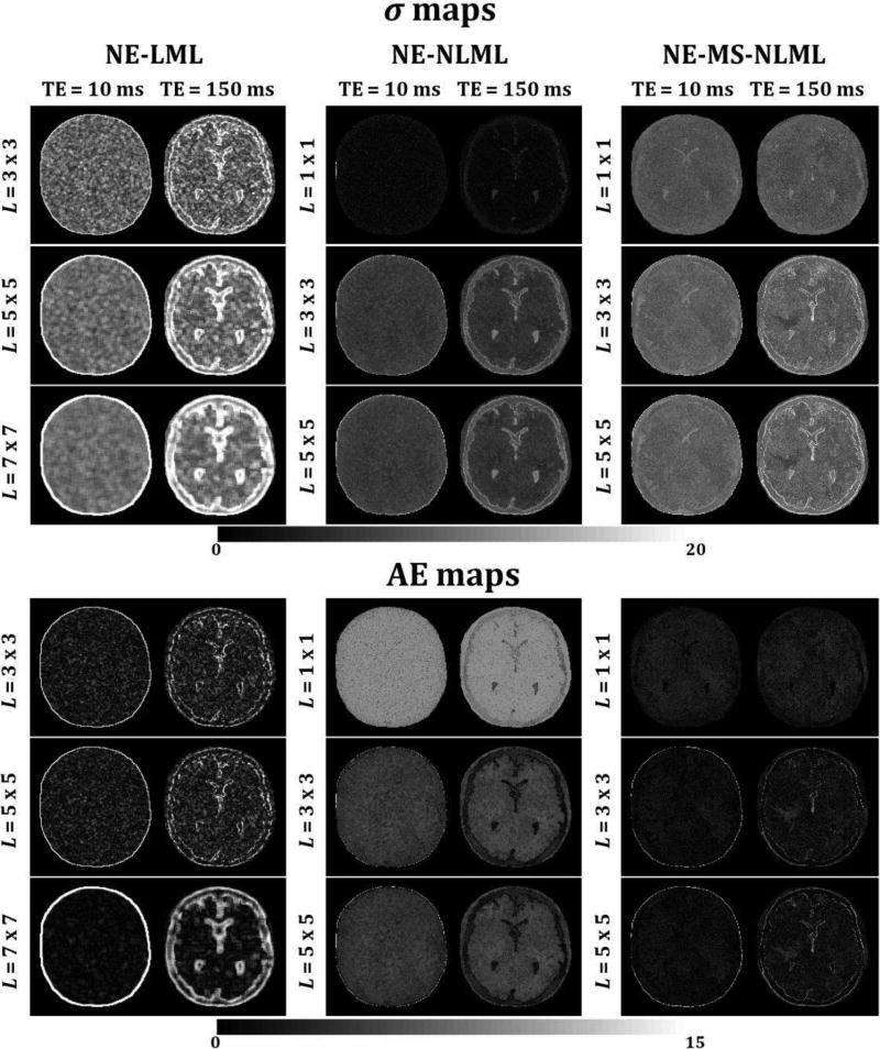
Fig. 1 shows the performance of the NE-LML, NE-NLML, and NE-MS-NLML methods for the estimation of σ, the noise SD. Analyses were performed on simulated noisy T₂W brain images with SNR = 10. The NE-LML method shows excellent performance especially at short TEs with relatively high SNR. This can be seen from the σ- and AE-maps exhibiting relatively low error. At long TE (i.e. low SNR) this method provides high performance only in the homogenous regions, with the performance clearly degraded in edge regions with rapidly varying intensities. This problem increases with increasing patch size. While the errors at edges were greatly reduced with NE-NLML, they remain substantial in the homogenous regions of the images, especially at long TEs. Finally, the NE-MS-NLML method demonstrated the highest performance for the determination of σ. This is clearly seen from the σ- and AE-maps showing very low errors in both edge and homogenous regions for all images obtained at different TEs. While increasing the patch size serves to decrease the performance of the method, especially at edges, this degradation remains negligible. Computational time requirements using a 2.6 GHz computer were ~3 hours for one complete dataset with K = 20 for each method.

Fig. 1.

Performance of NE-LML, NE-NLML, and NE-MS-NLML methods for noise estimation. Analyses were performed on simulated T₂W human brain images. σ and absolute error (AE) maps are displayed for two different echo times (TEs). For each method, analyses were performed for three different patch sizes. These results clearly indicate the superior performance of NE-MS-NLML for the determination of σ.

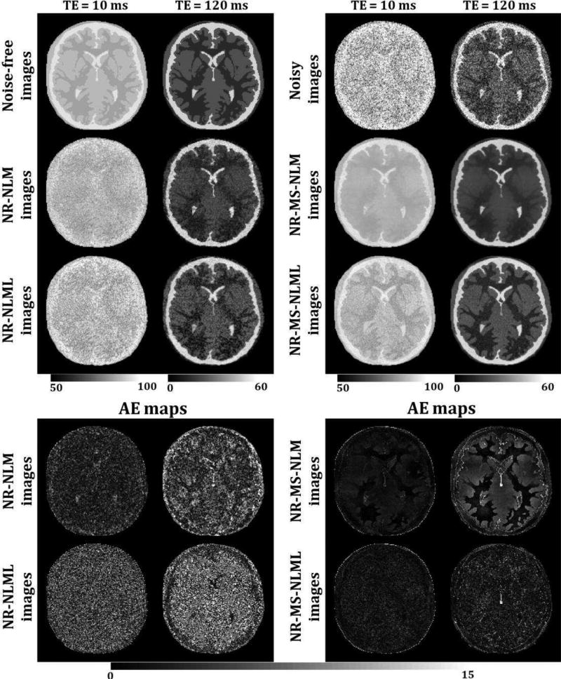
Fig. 2 shows qualitative and quantitative comparisons between marginal and multispectral filtering on simulated T₂W brain images obtained with SNR = 10. Both visual inspection of filtered images and AE-maps showed that all filters provided substantial reduction of noise. However, the multispectral filters, that is, NR-MS-NLM and NR-MS-NLML, exhibited minimal error compared to the marginal filters, that is, NR-NLM and NR-NLML. Although the error was low in the homogenous regions of the images using the NR-MS-NLM filter, it was very high at the edges, where intensities vary rapidly, and increased with decreasing SNR (i.e. increasing TE). In contrast, the error was very low in all spectral images and image regions, including edges, using the NR-MS-NLML filter, with images exhibiting minimal blurring and excellent preservation of detail. Total computation times using a 2.6 GHz computer were ~6 min, ~7 min, ~98 min and ~107 min for NR-NLM, NR-MS-NLM, NR-NLML, and NR-MS-NLML, respectively.

Fig. 2.

Comparison of marginal and multispectral filtering. Comparison of the performance of NR-NLM, NR-NLML, NR-MS-NLM and NR-MS-NLML filters was performed on simulated T₂W brain images. Noise-free, noisy and filtered images are displayed for two different TEs. For each TE, the windowing of gray levels was adjusted to compensate for signal loss. Absolute error (AE) maps are displayed for each filter and each TE. The windowing of gray levels was identical between different methods to ensure a direct comparison between different methods. The results clearly show the superior performance of the NR-MS-NLML filter.

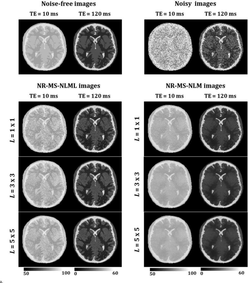
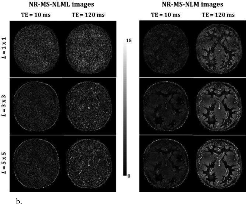
Fig. 3 shows qualitative (Fig. 3a) and quantitative (Fig. 3b) analyses of the effect of patch size on multispectral filtering. The performance of NR-MS-NLM and NR-MS-NLML were evaluated for three different patch sizes on simulated T₂W brain images obtained with SNR = 10. Visual inspection of filtered images shows that, unlike NR-MS-NLML, NR-MSNLM exhibits substantial blurring and loss of detail (Fig. 3a). This problem is exacerbated with increasing patch size as clearly seen from the AE-maps (Fig. 3b). In contrast, the NR-MS-NLML filter exhibits minimal blurring with preservation of detail, especially with patch size of L = 1 × 1 (i.e. no patch). Visual inspection of filtered images and AE-maps did show some persistent random variations due to the residual noise.

Fig. 3.

a. Evaluation of patch size effect on multispectral filtering. The performance of the NR-MS-NLM and NR-MS-NLML filters was evaluated on simulated T₂W brain images for three different patch sizes. Noise-free, noisy and filtered images are displayed for two different TEs. For each TE, the windowing of gray levels was adjusted to compensate for signal loss. The windowing of gray levels was identical between different methods to ensure a direct comparison between different methods.

b. Absolute error maps calculated from the noise-free and the filtered images obtained using the NR-MS-NLM or NR-MS-NLML filters for three different patch sizes. Results are shown for TEs that correspond to the images presented in Fig. 3a.

IV. 2. Experimental analysis

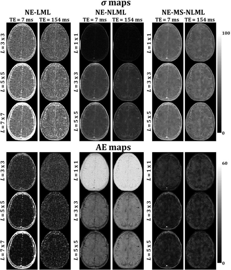
Figs. 4 shows the performance of the NE-LML, NE-NLML, and NE-MS-NLML methods for estimation of σ, the noise SD. Analyses were performed on in-vivo T₂W images obtained at different TEs. The NE-LML method performed well only in homogenous regions with clear performance degradation at the edges, especially with increasing patch size. While the error in the edges was greatly reduced with NE-NLML, it remains substantial in the homogenous regions of the images, especially at long TEs (i.e. low SNRs). Finally, the NE-MS-NLML method demonstrated the best performance for the determination of σ especially with patch size of 1 × 1 (i.e. no patch). Results were in good agreement with the numerical analysis shown in Fig. 1.

Fig. 4.

Performance of NE-LML, NE-NLML, and NE-MS-NLML methods for noise estimation. Analyses were performed on in-vivo T₂W human brain images. σ and absolute error (AE) maps are displayed for two different echo times (TEs). For each method, analyses were performed for three different patch sizes. The results clearly demonstrate the superior performance of NE-MS-NLML for the determination of σ.

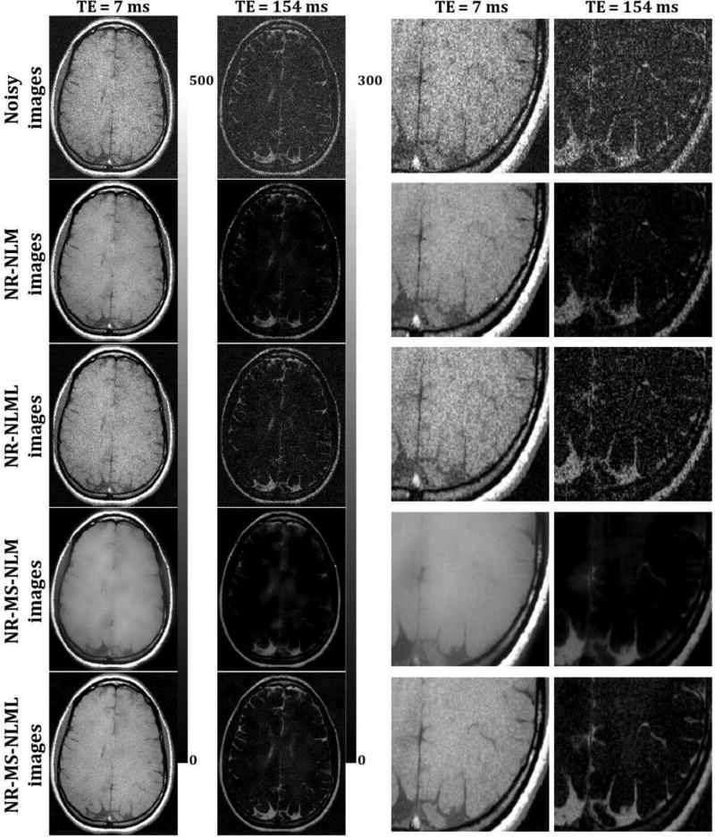
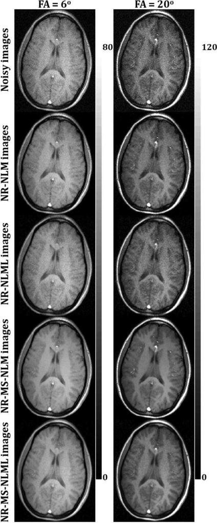
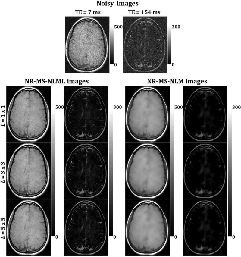
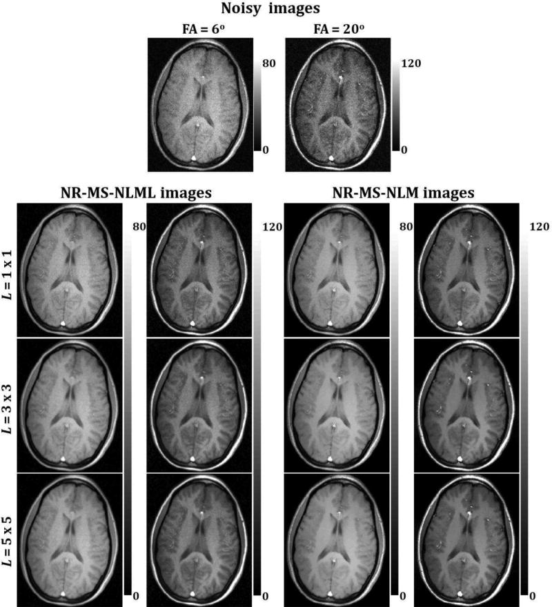
Figs. 5 and 7 show comparisons between marginal and multispectral filtering of in-vivo human brain images obtained at different TEs (Figs. 5) or FAs (Fig. 7). Visual inspection of filtered images showed that all of the filters provided substantial noise reduction. However, the multispectral filters, that is, NR-MS-NLM and NR-MS-NLML, demonstrated higher performance compared to the marginal filters, that is, NR-NLM and NR-NLML. However, unlike NR-MS-NLML, NR-MS-NLM suffers from visually apparent blurring and loss of image detail, as clearly visible from the filtered T₂W images in regions of rapidly varying intensity, especially at edges and within small structures (Fig. 5). This problem is exacerbated with increasing patch size (Fig. 6). In contrast, NR-MS-NLML exhibits minimal blurring with excellent preservation of detail, especially with a patch size of L = 1 × 1 (Figs. 6). Unlike T₂W images, T₁W images were less affected by noise and reflected high contrast between white and gray matter. This resulted in high image quality filtering with both NR-MS-NLM and NR-MS-NLML filters (Figs. 7–8).

Fig. 5.

Comparison of marginal and multispectral filtering. Comparison of the performance of NR-NLM, NR-NLML, NR-MS-NLM and NR-MS-NLML filters was performed on in-vivo T₂W human brain images. Noisy and filtered images are displayed for two different TEs. For each TE, the windowing of gray levels was adjusted to compensate for signal loss. The windowing of gray levels was identical between different methods to ensure a direct comparison between different methods. A zoomed region is displayed for each filter and each TE. The results clearly show the superior performance of the NR-MS-NLML filter.

Fig. 7.

Comparison of marginal and multispectral filtering. Comparison of the performance of NR-NLM, NR-NLML, NR-MS-NLM and NR-MS-NLML filters was performed on in-vivo T₁W human brain images. Noisy and filtered images are displayed for two different flip angles (FA). For each FA, the windowing of gray levels was adjusted to compensate for signal loss. The windowing of gray levels was identical to ensure a direct comparison between different methods.

Fig. 6.

Evaluation of the effect of patch size on multispectral filtering. The performance of the NR-MS-NLM and NR-MS-NLML filters was evaluated on in-vivo T₂W human brain images for three different patch sizes. Noisy and filtered images are displayed for two different TEs. For each TE, the windowing of gray levels was adjusted to compensate for signal loss. The windowing of gray levels was identical to ensure a direct comparison of different methods.

V. DISCUSSION

The presence of noise in MR images affects diagnostic accuracy, the quality of image manipulations such as registration and segmentation, and extraction of quantitative tissue information [1], [31]–[32], [36]–[40]. To partially overcome limitations imposed by noise, noise reduction filters may be applied during post-processing. However, filtering can introduce bias or produce blurring effects, affecting the accuracy of data analysis or obscuring small tissue structures. Further, noise SD is a crucial parameter in most filtering algorithms and requires careful estimation.

In the present study, we extended the LML estimation of noise to both the nonlocal and multispectral cases. In addition, we extended the NLML filter to the multispectral case. Extensive numerical and experimental analyses were conducted to evaluate the performance of these new noise estimation and reduction methods, with systematic comparison to existing and widely used methods. Through numerical and experimental analyses, we have demonstrated that the NE-MS-NLML method for the estimation of noise SD is more effective than both NE-LML and NE-NLML. In fact, while NE-LML showed excellent performance in homogenous regions, errors were large at edges due to partial volume effects. While this issue was attenuated with the NE-NLML filter, the error in the estimation of noise SD was considerable in homogenous regions due to the difficulty in determining similar patches between voxels, especially at low SNR. However, use of multispectral information with NE-MS-NLML allows more accurate determination of similar voxels, and hence higher quality estimation of noise SD (Figs. 1 and 4). In fact, voxels belonging to the same tissue have similar signal evolution as a function of frame number k, defined as a variation of a given acquisition parameter, such as TE, TR, FA or b-value. Likewise, comparison of different filters indicates the superior performance of multispectral filtering compared to marginal filtering. Thus, here as well, use of multispectral information allows more accurate determination of similar voxels. Moreover, our results showed that although patch-based similarity calculations provide optimal results in homogenous image regions (Figs. 3, 6 and 8), performance is limited in spatially heterogeneous regions, such as edges and small structures, where patch redundancy is relatively poor. Finally, while NR-MS-NLM showed substantial reduction of noise, NR-MS-NLML showed much higher performance with images exhibiting minimal blurring and excellent preservation of detail (Figs. 2, 3, 5, 6, 7 and 8). In fact, NR-MS-NLM is based on a weighted mean of signal intensities calculated between the voxel being filtered and all other voxels in a large search window. In the case of low contrast between tissues or low SNR, the calculated weights are likely to be inaccurate. This translates directly into incorporation of inappropriate pixels into the calculation of the estimated intensity of the pixel of interest, leading to, in effect, partial volume effects. This is seen as blurring of the filtered images (Figs. 2, 3, 5 and 6). In contrast, NR-MS-NLML uses only similar voxels to restore the amplitude of the voxel being analyzed.

Fig. 8.

Evaluation of the effect of patch size on multispectral filtering. The performance of the NR-MS-NLM and NR-MS-NLML filters was evaluated on in-vivo T₁W human brain images for three different patch sizes. Noisy and filtered images are displayed for two different flip angles (FA). For each FA, the windowing of gray levels was adjusted to compensate for signal loss.

NE-MS-NLML and NR-MS-NLML achieve noise estimation or reduction using multispectral amplitude values from M similar voxels, where M is user-defined. The value of M needs to be carefully selected. We observed suboptimal denoising for relatively small values of M. In addition, larger values of M degrade the quality of noise estimation or reduction by including voxels that are progressively less similar to the voxel being analyzed. Adaptive selection of M is therefore advantageous and may be performed following the methodology described in [33], at the expense of further increase in processing time. Likewise, NR-MS-NLM requires appropriate selection of the smoothing parameter h. While it has been established that noise SD can represent an optimal value for h, our analysis showed that this parameter is highly dependent on SNR and contrast between tissues (Figs. 2–3, 5–8.

Finally, although we compared all noise estimation and reduction methods using a 2D implementation, that is, voxel similarities were calculated in a single slice, these methods can readily be extended to 3D data sets at the expense of increased processing time. Moreover, we have used the Rician distribution, as is appropriate for single-coil signal reception. Multiple receiver coils are widely used to increase speed or SNR. If uncorrelated and equally distributed noise is assumed, the noise distribution in the resulting magnitude images is described by generalizations of the Rician, known as noncentral χ-distributions. Even if correlations do exist between different coils, the non-central χ-distributions can still be assumed, using pre-calculated effective values for the number of coils and noise SD, as described in [41].

In conclusion, we have presented efficient methods for noise estimation and reduction in multispectral MR images. Extensive numerical and experimental analyses indicate that the methods introduced show overall improved performance compared to other well-established methods.

References

- 1.Feng Y, He T, Feng M, Charpenter JP, Greiser A, Xin X, Chen W, Pennell DJ, Yang GZ, Firmin DN. Improved pixel-by-pixel MRI R2* Relaxometry by nonlocal means. Magn. Reson. Med. 2014;72(1):260–268. doi: 10.1002/mrm.24914. [DOI] [PubMed] [Google Scholar]
- 2.Perona P, Malik J. Scale-space and edge-detection using anisotropic diffusion. IEEE Trans. Pattern. Anal. Mach. Intell. 1990;12(7):629–639. [Google Scholar]
- 3.Samsonov AA, Johnson CR. Noise-adaptive nonlinear diffusion filtering of MR images with spatially varying noise levels. Magn. Reson. Med. 2004;52(4):798–806. doi: 10.1002/mrm.20207. [DOI] [PubMed] [Google Scholar]
- 4.Buades A, Coll B B, Morel JM. A review of image denoising algorithms, with a new one. Multiscal. Mod. Sim. 2005;4(2):490–530. [Google Scholar]
- 5.Liu H, Yang CH, Pan N, Song EM, Green R. Denoising 3D MR images by the enhanced nonlocal means filter for Rician noise. Magn. Reson. Imag. 2010;28(10):1485–1496. doi: 10.1016/j.mri.2010.06.023. [DOI] [PubMed] [Google Scholar]
- 6.Manjon JV, Coupe P, Marti-Bonmati L, Collins DL, Robles M. Adaptive nonlocal means denoising of MR images with spatially varying noise levels. J. Magn. Reson. Imag. 2010;31(1):192–203. doi: 10.1002/jmri.22003. [DOI] [PubMed] [Google Scholar]
- 7.Tomasi C, Manduchi R. Bilateral filtering for gray and color images; Proc 6th Intern. Conf. Comput. Vis; 1998. pp. 839–846. [Google Scholar]
- 8.Wong WCK, Chung ACS, Yu SCH. Trilateral filtering for biomedical images; Proc. IEEE Intern. Symp. Biomed. Imag: From Macro to Nano; 2004. pp. 820–823. [Google Scholar]
- 9.Anand CS, Sahambi JS. Wavelet domain nonlinear filtering for MRI denoising. Magn. Reson. Imag. 2010;28(6):842–861. doi: 10.1016/j.mri.2010.03.013. [DOI] [PubMed] [Google Scholar]
- 10.Delakis I, Hammad O, Kitney RI. Wavelet-based de-noising algorithm for images acquired with parallel magnetic resonance imaging (MRI) Phys. Med. Biol. 2007;52:3741–751. doi: 10.1088/0031-9155/52/13/006. [DOI] [PubMed] [Google Scholar]
- 11.Donoho DL, Johnstone IM. Ideal spatial adaptation by wavelet shrinkage. Biometrika. 1994;81(3):425–455. [Google Scholar]
- 12.Nowak RD. Wavelet-based Rician noise removal for magnetic resonance imaging. IEEE Trans. Imag. Process. 1999;8(10):1408–1419. doi: 10.1109/83.791966. [DOI] [PubMed] [Google Scholar]
- 13.Weaver JB, Xu YS, Healy DM, Cromwell LD. Filtering noise from images with wavelet transforms. Magn. Reson. Med. 1991;21(2):288–295. doi: 10.1002/mrm.1910210213. [DOI] [PubMed] [Google Scholar]
- 14.Wink AM, Roerdink JB. Denoising functional MR images: a comparison of wavelet denoising and Gaussian smoothing. IEEE Trans. Med. Imag. 2004;23(3):374–387. doi: 10.1109/TMI.2004.824234. [DOI] [PubMed] [Google Scholar]
- 15.Wood JC, Johnson KM. Wavelet packet denoising of magnetic resonance images: importance of Rician noise at low SNR. Magn. Reson. Med. 1999;41(3):631–635. doi: 10.1002/(sici)1522-2594(199903)41:3<631::aid-mrm29>3.0.co;2-q. [DOI] [PubMed] [Google Scholar]
- 16.Zaroubi S, Goelman G. Complex denoising of MR data via wavelet analysis: application for functional MRI. Magn. Reson. Imag. 2000;18(1):59–68. doi: 10.1016/s0730-725x(99)00100-9. [DOI] [PubMed] [Google Scholar]
- 17.He L, Greenshields IR. A nonlocal maximum likelihood estimation method for Rician noise reduction in MR images. IEEE Trans. Med. Imag. 2009;28(2):165–172. doi: 10.1109/TMI.2008.927338. [DOI] [PubMed] [Google Scholar]
- 18.Rajan J, den Dekker AJ, Juntu J, Sijbers J. A new nonlocal maximum likelihood estimation method for denoising magnetic resonance images. Pattern Recognit. Mach. Intell. 2013;8251:451–458. [Google Scholar]
- 19.Rajan J, Jeurissen B, Verhoye M, Van Audekerke J, Sijbers J. Maximum likelihood estimation-based denoising of magnetic resonance images using restricted local neighborhoods. Phys. Med. Biol. 2011;56(16):5221–5234. doi: 10.1088/0031-9155/56/16/009. [DOI] [PubMed] [Google Scholar]
- 20.Rajan J, Veraart J, Van Audekerke J, Verhoye M, Sijbers J. Nonlocal maximum likelihood estimation method for denoising multiple-coil magnetic resonance images. Magn. Reson. Imag. 2012;30(10):1512–1518. doi: 10.1016/j.mri.2012.04.021. [DOI] [PubMed] [Google Scholar]
- 21.Kosior JC, Kosior RK, Frayne R. Robust dynamic susceptibility contrast MR perfusion using 4D nonlinear noise filters. J. Magn. Reson. Imag. 2007;26:1514–1522. doi: 10.1002/jmri.21219. [DOI] [PubMed] [Google Scholar]
- 22.Keeling SL. Total variation based convex filters for medical imaging. Appl. Math. Comput. 2003;139(1):101–119. [Google Scholar]
- 23.Mohan J, Krishnaveni V, Guo YH. A survey on the magnetic resonance image denoising methods. Biomed. Sign. Process. Control. 2014;9:56–69. [Google Scholar]
- 24.Manjón JV, Thacker NA, Lull JJ, Garcia-Martí GG, Martí-Bonmatí L, Robles M. Multicomponent MR Image Denoising. Int. J. Biomed. Imag. 2009 doi: 10.1155/2009/756897. Article ID 756897. [DOI] [PMC free article] [PubMed] [Google Scholar]
- 25.Manjón JV, Robles M, Thacker N. Proc. MIUA’07. Aberystwyth, Wales: 2007. Multispectral MRI denoising using non-local means; pp. 41–45. [Google Scholar]
- 26.Wiest-Daesslé N, Prima S, Coupe P, Morrissey SP, Barillot C. Nonlocal means variants for denoising of diffusion-weighted and diffusion tensor MRI. Med. Imag. Comput. Comput. Assist. Interv. 2007;10(2):344–351. doi: 10.1007/978-3-540-75759-7_42. [DOI] [PMC free article] [PubMed] [Google Scholar]
- 27.Zhou MX, Yan X, Xie HB, Zheng H, Xu D, Yang G. Evaluation of nonlocal means based denoising filters for diffusion kurtosis imaging using a new phantom. PLoS One. 2015;10(2):e0116986. doi: 10.1371/journal.pone.0116986. [DOI] [PMC free article] [PubMed] [Google Scholar]
- 28.Aja-Fernández S, Alberola-López C, Westin CF. Noise and Signal Estimation in Magnitude MRI and Rician Distributed Images: A LMMSE Approach. IEEE Trans. Imag. Process. 2008;17:1383–1398. doi: 10.1109/TIP.2008.925382. [DOI] [PubMed] [Google Scholar]
- 29.Sijbers J, Poot D, den Dekker AJ, Pintjens W. Automatic estimation of the noise variance from the histogram of a magnetic resonance image. Phy. Med. Biol. 2007;52:1335–1348. doi: 10.1088/0031-9155/52/5/009. [DOI] [PubMed] [Google Scholar]
- 30.Sijbers J, den Dekker AJ. Maximum Likelihood Estimation of Signal Amplitude and Noise Variance From MR Data. Magn. Reson. Med. 2004;51:586–594. doi: 10.1002/mrm.10728. [DOI] [PubMed] [Google Scholar]
- 31.Bouhrara M, Reiter DA, Spencer RG. Bayesian analysis of transverse signal decay with application to human brain. Magn. Reson. Med. 2015;74(3):785–802. doi: 10.1002/mrm.25457. [DOI] [PMC free article] [PubMed] [Google Scholar]
- 32.Bouhrara M, Reiter DA, Celik H, Bonny JM, Lukas V, Fishbein KW, Spencer RG. Incorporation of Rician noise in the analysis of biexponential transverse relaxation in cartilage using a multiple gradient echo sequence at 3 and 7 Tesla. Magn. Reson. Med. 2015;73(1):352–366. doi: 10.1002/mrm.25111. [DOI] [PMC free article] [PubMed] [Google Scholar]
- 33.Rajan J, Van Audekerke J, Van der Linden A, Verhoye M, Sijbers J. An adaptive non local maximum likelihood estimation method for denoising magnetic resonance images. ISBI. 2012:1136–1139. doi: 10.1016/j.mri.2012.04.021. [DOI] [PubMed] [Google Scholar]
- 34.Buades A, Coll B, Morel JM. A nonlocal algorithm for image denoising; IEEE Comput. Soc. Conf. Comput. Vis. Pattern. Recognit. Proc; 2005. pp. 60–65. [Google Scholar]
- 35.Wiest-Daessle N, Prima S, Coupe P, Morrissey SP, Barillot C. Rician noise removal by nonLocal Means filtering for low signal-to-noise ratio MRI: applications to DT-MRI. Med. Imag. Comput. Comput. Assist. Interv. 2008;11(2):171–179. doi: 10.1007/978-3-540-85990-1_21. [DOI] [PMC free article] [PubMed] [Google Scholar]
- 36.Chen GY, Coulombe S. A new image registration method robust to noise. Multidim. Sys. Sign. Process. 2014;25:601–609. [Google Scholar]
- 37.Despotovic I, Jelaca V, Vansteenkiste E, Philips W. Noise-Robust Method for Image Segmentation. Adv. Concepts Intell. Vis. Sys. 2010;6474:153–162. [Google Scholar]
- 38.Bouhrara M, Spencer RG. Improved determination of the myelin water fraction in human brain using magnetic resonance imaging through Bayesian analysis of mcDESPOT. NeuroImage. 2016;127:456–471. doi: 10.1016/j.neuroimage.2015.10.034. [DOI] [PMC free article] [PubMed] [Google Scholar]
- 39.Bouhrara M, Reiter DA, Celik H, Fishbein KW, Kijowski R, Spencer RG. Analysis of mcDESPOT- and CPMG-derived parameter estimates for two-component nonexchanging systems. Magn. Reson. Med. 2016;75:2406–2420. doi: 10.1002/mrm.25801. [DOI] [PMC free article] [PubMed] [Google Scholar]
- 40.Celik H, Bouhrara M, Reiter DA, Fishbein KW, Spencer RG. Stabilization of the inverse Laplace transform of multiexponential decay through introduction of a second dimension. J. Magn. Reson. 2013;236:134–139. doi: 10.1016/j.jmr.2013.07.008. [DOI] [PMC free article] [PubMed] [Google Scholar]
- 41.Aja-Fernández S, Brionb V, Tristán-Vega A. Effective noise estimation and filtering from correlated multiple-coil MR data. Magn. Reson. Imag. 2013;31:272–285. doi: 10.1016/j.mri.2012.07.006. [DOI] [PubMed] [Google Scholar]