Low-Dose CT Perfusion of the Liver using Reconstruction of Difference

Abstract

Liver CT perfusion (CTP) is used in the detection, staging, and treatment response analysis of hepatic diseases. Unfortunately, CTP radiation exposures is significant, limiting more widespread use. Traditional CTP data processing reconstructs individual temporal samples, ignoring a large amount of shared anatomical information between temporal samples, suggesting opportunities for improved data processing. We adopt a prior-image-based reconstruction approach called Reconstruction of Difference (RoD) to enable low-exposure CTP acquisition. RoD differs from many algorithms by directly estimating the attenuation changes between the current patient state and a prior CT volume. We propose to use a high-fidelity unenhanced baseline CT image to integrate prior anatomical knowledge into subsequent data reconstructions. Using simulation studies based on a 4D digital anthropomorphic phantom with realistic time-attenuation curves, we compare RoD with conventional filtered-backprojection, penalized-likelihood estimation, and prior image penalized-likelihood estimation. We evaluate each method in comparisons of reconstructions at individual time points, accuracy of estimated time-attenuation curves, and in an analysis of common perfusion metric maps including hepatic arterial perfusion, hepatic portal perfusion, perfusion index, and time-to-peak. Results suggest that RoD enables significant exposure reductions, outperforming standard and more sophisticated model-based reconstruction, making RoD a potentially important tool to enable low-dose liver CTP.

I. Introduction

CT perfusion (CTP) is a functional imaging modality that measures the tissue blood-flow parameters through sequential CT scanning of the same tissue or organ over the time. Typically, an iodinated contrast agent is administered and projection images are acquired before, during, and after injection of contrast to track temporal changes in CT attenuation. With the availability of wide-area detectors (e.g. 256 slices or more), CT can cover whole organs which has facilitated CTP in a variety of applications including head and neck, liver, lung and colorectal imaging [1]. CTP has shown remarkable results in diagnosing malignant and non-malignant parotid lesions [2] and in assessing tumor vascularity changes that result from chemotherapy and radiation therapy [3].

Liver CT perfusion provides valuable information on blood flow dynamics in the assessment of liver damage or severity of hepatic fibrosis in patients with chronic liver disease [4], in the evaluation of therapeutic effectiveness for liver cancer [5], and in the assessment of hepatic perfusion changes after surgical and radiological interventions [6], [7]. Recent studies also revealed promising results of using CTP as a viable biomarker for of hepatocellular carcinoma (HCC) tumor and pancreatic lesion detection and analysis [8], [9].

Despite the clinical utility of the CTP, the radiation dose associated with sequential scanning is a major concern that has limited more widespread adoption in both clinical and research applications [10], [11]. CTP studies involve many repeat acquisitions (e.g., often ~20 time points) representing a significant radiation exposure. Several methods have been proposed to reduce exposures including customization of scanning parameters (e.g., tube current or voltage) to the size of the patient and variation of exposure throughout the temporal evolution [12]–[15]. However, lowering x-ray exposure, inevitably reduces the quality of the CT images and can introduce errors including noise and streak artifacts which, in turn, decreases the accuracy of the perfusion metrics limiting clinical utility.

Model-based iterative reconstruction (MBIR) techniques have been introduced as a potential solution to improve the trade-off between radiation exposure and image quality. Recent studies on body CT scanning have demonstrated that such advanced processing methods can maintain image quality at lower exposures, thereby enabling lower effective dose to the patient [16], [17]. Negi et al. [18] investigated iterative image reconstruction methods and hepatic CTP analysis where they found that adaptive iterative dose reduction (AIDR) reduced the image noise while maintaining hepatic perfusion parameters values.

Such MBIR approaches significantly improve the dose-image quality trade-off through statistical modeling of the measurement data (i.e., effectively downweighting measurements with poor signal-to-noise and upweighting measurements with good signal-to-noise) as well as sophisticated image regularization (e.g., applying constraints or penalties that enforce smoothing with edge-preservation). However, most reconstruction methods tend to be applied in isolation, neglecting the large amount of shared information between scans.

In contrast, prior-image-based reconstruction (PIBR) approaches have been introduced that explicitly incorporate patient-specific anatomical information found in previously acquired scans. Such information is arguably much stronger than traditional assumptions of image smoothness and should allow for further reductions of noise and artifacts over conventional MBIR regularization. Prior-image-constrained compressed sensing (PICCS) is one well-known PIBR approach that has been used to integrate high quality prior information to reconstruct tomographic volumes from under-sampled projection data [19]. PICCS has also demonstrated success in small animal CTP [20]. The prior image registration penalized-likelihood estimation (PIRPLE) method [21] combines both patient-specific prior information and statistical modeling within an objective function that seeks both reconstruction of the tomographic volume as well as registration of the prior image. A variant of this approach with deformable registration, dPIRPLE [22] has also been presented and applied to the clinical scenario of low-dose lung nodule screening, demonstrating the capability for dramatic reductions in exposure. More recently, Pourmorteza et al. [23] proposed a novel PIBR method called Reconstruction of Difference (RoD). This technique borrows an idea from 2D digital subtraction angiography where it is not the current anatomical state that is of greatest interest, but the change in state from a previous time point. That is, rather than attempting to estimate the current tomographic image volume, only the difference between the current anatomical state and a prior state is estimated. In the context of CTP, one can focus on reconstructing only the contrast enhancement itself. Previous work [23] has suggested that such processing can limit structured noise and can allow smaller reconstruction volumes focused only on the region-of-change (as opposed to the entire patient volume).

In this paper, we investigate the feasibility of applying the RoD technique for liver CT perfusion. Specifically, this work studies the ability to reconstruct difference images between a high-quality unenhanced baseline image (the prior image) and subsequent contrast-enhanced images which are acquired in a low dose setting. The work presented here is a more complete presentation of the preliminary work presented in [24] and includes expanded investigations on optimal regularization, sensitivity to exposure levels, and an additional perfusion metric. Similarly, this work includes investigations and comparisons to another prior image based reconstruction technique (PIPLE). Assessments were based in simulation studies where ground truth is known. A realistic 4D digital liver phantom was adopted using time-attenuation curves (TAC) based on dynamics derived from a rabbit animal model with both healthy and cancerous tissues. RoD was compared to traditional analytic and MBIR approaches across a range of simulated exposures to assess the potential for dose reduction. Reconstruction methods were evaluated on their ability to accurately reconstruct TACs as well as specific hepatic perfusion metrics including hepatic arterial perfusion (HAP), hepatic portal perfusion (HPP), perfusion index (PI) and time-to-peak (TTP).

II. Methods

A. Overview of the Proposed RoD Methodology

The proposed data processing chain for CTP image reconstruction using the RoD technique is shown in Figure 1. A key feature of this approach is the use of a high-fidelity unenhanced baseline image as a prior image (μ_p) in the reconstruction of subsequent sequentially measured CT data (y) during and after contrast administration. The RoD approach directly reconstructs a difference image (μ_Δ) representing the contrast enhancement of the liver and other tissues in each time point (t_n) relative to the baseline reconstruction. Representations of the current anatomy $(\widehat{\mu })$ may be formed by adding the prior image to the difference estimate. From these estimates, time-attenuation curves and common liver CTP metrics like hepatic arterial perfusion (HAP), hepatic portal perfusion (HPP), perfusion index (PI), and time-to-peak (TTP) can be computed.

Figure 1.

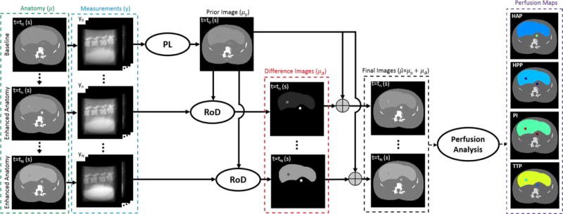
Overview of the proposed data acquisition, reconstruction and processing chain for liver CT perfusion using RoD. A high-quality baseline image based on a normal exposure acquisition and penalized-likelihood reconstruction serves as a prior image for subsequent RoD processing. Low dose tomographic data is acquired for a series of time points following injection of a contrast agent and differences image volumes are formed using RoD for each time point in the series. Estimates of the current anatomy may be obtained by adding the difference images to the prior image, permitting standard methods to be applied to generate perfusion maps including hepatic arterial perfusion (HAP), hepatic portal perfusion (HPP), perfusion index (PI), and time-to-peak (TTP).

The following sections detail CTP data generation using a dynamic digital liver phantom, the RoD objective function and reconstruction methods for comparison, as well as perfusion metric analysis and evaluation methods.

B. Anatomical Model for Liver CT Perfusion

Simulation studies require a realistic anatomical model to evaluate the potential for dose reduction. This model serves as the ground truth for algorithm comparisons as well as data generation. The following subsections outline the process used to develop a realistic 4D liver perfusion phantom.

1) Time-Attenuation Curves from an Animal Model

For this work, we obtained realistic TACs from an animal model. Specifically, an adult male New Zealand white rabbit (3.5 kg) was selected for the study. The animal was implanted with a VX2 tumor in the left lobe of the liver using previously documented procedures [25], [26] and allowed to grow for 13-15 days prior to CTP imaging. The rabbit was sedated using ketamine (20 mg/kg) and xylazine (8 mg/kg) via intramuscular injection. CTP studies were acquired using an Aquilion ONE (Toshiba, Japan) 320-slice CT scanner with a 22-cm field-of-view and x-ray technique of 120 kVp and 80 mA. Contrast agent (1.5 ml/kg, 320 I/ml Visipaque, GE Healthcare, Princeton, NJ) was administered at 1 ml/second via a marginal ear vein followed by a 7-ml saline flush at 1 ml/second.

Following a 6-sec delay, CT data was acquired at 2-sec intervals for 25 seconds, followed by 3-second intervals for 42 seconds. Each scan took 0.5 seconds for a total of 17.5 seconds of scan time (CTDIvol = 164.7 mGy). CT reconstruction was performed using AIDR 3D (Toshiba Medical Systems, Japan) with 0.349 mm voxels. To compensate for breathing motion, CT dataset were registered using Body Registration (Toshiba Medical Systems, Tochigi, Japan).

Regions-of-interest (ROI) were identified within the aorta, portal vein, spleen, healthy liver tissue, and the liver tumor. Attenuation was averaged over the region to form raw TAC samples. A smoothing spline function [27], [28] was used to fit the liver perfusion TACs to reduce noise in the estimates. The resulting TACs for each region are shown in Figure 2.

Figure 2.

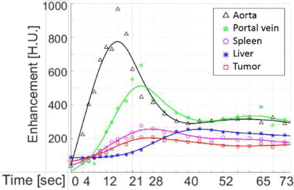
Time-attenuation curves from the contrast-enhanced rabbit abdominal study. Regions of interest covered the standard locations used to derive perfusion metrics and included five tissue types: the aorta, portal vein, spleen, healthy liver tissue, and a liver tumor.

2) Data Acquisition Protocol

The TACs in Figure 2 were used to generate simulated data via simple sampling of each curve. For simulation studies the temporal sampling followed a similar protocol as that used in the animal model with denser sampling at the beginning of the sequence. Specifically, an initial non-enhanced scan is acquired at t=0 when contrast injection starts. Subsequent scanning follows after a 4-second delay with 7 scans over 12 seconds, followed by a 6-second delay; then 10 scans over 28 seconds, a 5-second delay, and finally 5 scans over 16 seconds. These temporal samples are illustrated in Figure 3.

Figure 3.

Acquisition protocol used for CT perfusion studies.

3) 4D Dynamic Digital Liver Phantom

To assess performance in human CTP, a digital anthropomorphic phantom was generated. This phantom was based on a segmented physical phantom where different tissues types have been labeled. The TACs described in previous subsections were mapped onto different tissue types. Specifically, the healthy liver TAC was mapped onto the segmented liver, the aorta TAC was mapped onto the aorta, and two simulated spherical tumors was created using the tumor TAC. The first tumor (marked red in Figure 4) was homogeneous with a sharp edge profile while the second one (marked green in Figure 4) has flat interior profile with a smooth edge based on a Gaussian profile. Both lesions have the same full-width half-maximum of 3.2 mm. The 4D digital phantom is shown in Figure 4 for several time points. The images show the entire abdominal area including liver as well as zoomed ROIs around the simulated spherical homogeneous and Gaussian lesions. The variable enhancement of the liver, tumor, and aorta is illustrated in axial images. Constant attenuation regions (bone, other soft-tissues) were set equal to the attenuation values in the original physical phantom data.

Figure 4.

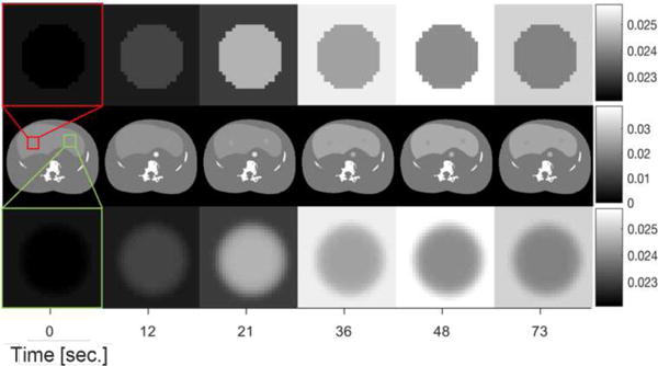
4D Digital liver phantom designed for CT perfusion studies. Middle row illustrates the entire abdominal area including liver, first row and third row include the zoomed regions around a simulated homogeneous lesion and a Gaussian lesion respectively for several time points.

C. Forward Model for Data Generation

We adopt a simple monoenergetic forward model for our experiments. The mean measurements in this transmission tomography model are written:

$${\overline{y}}_i=I_0\exp (-{[\mathbf{A}\mu (t)]}_i),$$ (1)

where I₀ denotes a scalar value associated with a uniform bare-beam fluence, measured in (x-ray) photons. We presume that measurements, y_i, are independent and Poisson distributed (e.g., readout noise is negligible and noise is dominated by x-ray shot noise). Thus, the exposure level in the data is given by I₀. The vector μ(t) denotes the vector of attenuation coefficients in the anatomical volume at a given time point. (In subsequent equations we drop the dependence on t for simplicity and since we presume that attenuation values are constant over the scan and reconstructions only involve estimation of the current single-time-point image volume, or a difference volume). The projection operation is denoted by A and [Aμ]_i is the line integral associated with the i^th measurement. To MODEL partial volume effects in the data generation model, we have an intentional mismatch where the phantom volume is sampled at 2x the reconstruction voxel size, and linear projections (A) are also computed at 2x the sampling of the detector pixel size (with subsequent downsampling post-exponentiation to match the pixel size). All data simulations used a common CT geometry summarized in Table I and projection data were formed with a separable footprints projector [29].

TABLE I.

Simulation parameters

Quantity	Value
Rotation Angle	360 degrees
Volume Size	512×512×64
Voxel Size	0.4 mm
Number of Projections	360
Source-to-Axis Distance	1000 mm
Source-to-Detector Distance	500 mm
Detector Pixel Size	1 mm × 1mm

D. Reconstruction Methods

Four different reconstruction methods are applied to the data. These methods are outlined in the following subsections.

1) Feldkamp–Davis–Kress Reconstruction

For a baseline analytic reconstruction we used the Feldkamp–Davis–Kress (FDK) algorithm [30] which is a commonly used method for direct CT reconstruction. Data was prepared using ideal gain correction, logarithmic transformation, and thresholding of the data at 10⁻⁴. The reconstruction used a ramp filter apodized with a raised cosine function [31] with a cutoff frequency of 0.8 times Nyquist. This cutoff frequency was chosen to optimize FBP performance in terms of root mean-squared error (RMSE) in the reconstructed images.

2) Penalized-Likelihood (PL) Reconstruction

To investigate performance using a well-known MBIR approach we adopted a penalized-likelihood estimator [32]. The objective function for this reconstruction may be written as

$$\varphi (\mu ;y)=-L(\mu ;y)+\beta \left|\right|\mu \left|\right|,$$ (2)

where L represents the log-likelihood function which is derived using the Poisson likelihood assumption and a data model matching (1). The second term in (2) is a traditional edge-preserving roughness penalty term. The operator Ψ denotes a local pairwise voxel difference operator and, in this work, we will choose to implement ||·|| using a Huber cost function [33]. The regularization parameter β controls the balance between the data fidelity and roughness penalty controlling the noise-resolution trade-off. The optimization problem can be written as

$$\widehat{\mu }=\arg \underset{\mu \in {\mathrm{ℝ}}^{N_{\mu }}}{min}\varphi (\mu ;y).$$ (3)

We solve this objective iteratively using the separable quadratic surrogates approach [34] using 100 iterations and 10 subsets.

3) Prior Image Penalized-Likelihood Estimation (PIPLE)

To investigate performance using a prior image based MBIR approach we implemented a PIPLE as described in [21] which has the following objective function

$$\varphi (\mu ;y)=-L(\mu ;y)+{\beta }_R\left|\right|\mathbf{\Psi }\mu \left|\right|+{\beta }_P\left|\right|\mu -{\mu }_{\mathrm{p}}\left|\right|,$$ (4)

with the same log-likelihood function and traditional roughness penalty as (2). The third term is a prior image penalty with μ_p denoting the prior image. The parameters β_R and β_P denote the relative strengths of the roughness and prior image penalty respectively. The optimization has the same form as (3) and is solved using the separable quadratic surrogates (SPS) algorithm [33]. For PIPLE, 100 iterations and 10 subsets were used.

4) Reconstruction of Difference

The Reconstruction of Difference (RoD) algorithm [23] is summarized briefly as follows. Rather than reconstruct the current anatomy (μ), RoD aims to reconstruct the difference between the current anatomical volume and a prior image volume. In the case of CT perfusion imaging, RoD can be employed to reconstruct the contrast change – that is, the difference image volume (μ_Δ) – between the unenhanced baseline, or prior image (μ_p), and an enhanced image volume (μ) at a later time point. Specifically, we may write

$$\mu ={\mu }_{\mathrm{p}}+{\mu }_{\mathrm{\Delta }}.$$ (5)

Substituting (4) in forward model (1), one can rewrite the mean measurements model as

$$\overline{y}=[I_0\exp (-\mathbf{A}{\mu }_{\mathrm{p}})]\cdot \exp (-\mathbf{A}{\mu }_{\mathrm{p}})=g\cdot \exp (-\mathbf{A}{\mu }_{\mathrm{\Delta }}).$$ (6)

where L represents the log-likelihood function which is derived using the Poisson likelihood assumption. The Poisson assumption is commonly applied and is based on measurement noise being dominated by x-ray quantum noise. Note that this new forward model can be rewritten in the second equality with the gain term g. This gain is mathematically equivalent to (1) where the scalar I₀ has been replaced with element-by-element multiplication by the vector g and, and μ has been replaced by μ_Δ. Because of the similar form, it is straightforward to write a new objective and algorithm based on this difference model. Specifically, using a likelihood-based objective function for difference image, μ_Δ, we may write:

$$\varphi ({\mu }_{\mathrm{\Delta }};y,{\mu }_{\mathrm{p}})=-L({\mu }_{\mathrm{\Delta }};y,{\mu }_{\mathrm{p}})+{\beta }_R\left|\right|\mathbf{\Psi }{\mu }_{\mathrm{\Delta }}\left|\right|+{\beta }_M\left|\right|{\mu }_{\mathrm{\Delta }}\left|\right|.$$ (7)

Again, the log-likelihood function has the same basic form but with the difference model of (6). The second term is analogous to the standard roughness penalty in (2) except it is applied to the difference image. The third regularization term is a magnitude penalty on μ_Δ, which discourages too much change between the current anatomy and the prior image. In effect, this is the term that controls (via β_M) the degree of prior information integrated into the reconstruction. In the original formulation in [23] both penalties were presented as 1-norms. This is important, particularly for the third term which discourages change but permits sparse changes when a 1-norm is applied. However, in practice both penalties are computed using the Huber penalty (which maintains a differentiable objective function and a common iterative solver to the penalized-likelihood approach). The optimization of the objective is written simply as

$${\mu }_{\mathrm{\Delta }}=\arg \underset{{\mu }_{\mathrm{\Delta }}\in {\mathrm{ℝ}}^{N_{\mu }}}{min}\varphi ({\mu }_{\mathrm{\Delta }};y,{\mu }_{\mathrm{p}})$$ (8)

and like the other MBIR methods is solved using the separable quadratic surrogates (SPS) algorithm [34]. For RoD, 100 iterations and 10 subsets were used.

The number of iterations for RoD, PIPLE and PL was chosen in a convergence study which suggested that the image changes after 100 iterations were insignificant (specifically changes between iterations were less than 0.1 HU). The number of subsets (ten) were selected empirically as a good tradeoff between reconstruction speed and small reconstruction errors in the converged images. All reconstruction methods and related routines were written in Matlab (The Mathworks, Natick, MA) with external calls to projectors/back-projectors written in C/C++ using CUDA libraries to accelerate computations through the use of graphical processing units (GPUs).

E. Hepatic Perfusion Analysis

In addition to direct investigations on the accuracy of TACs produced by various methods, we investigate the ability to accurately estimate commonly used perfusion metrics. Those metrics are described briefly here. Because of the liver has two vascular inputs (e.g., unlike brain perfusion), hepatic CT perfusion analysis is more challenging than the perfusion parameters calculation for the other tissues. This dual input model is illustrated in Figure 5. In this work, we use dual-input maximum slope method (SM) to calculate the perfusion parameters as previously described by Miles et al. [35], [36]. The principle of the SM is quite simple which makes it very attractive for separate evaluation of dual liver blood supply components, i.e. hepatic arterial perfusion (HAP) and hepatic portal perfusion (HPP).

Figure 5.

Dual input liver perfusion model. C_a(t), C_p(t) and C_l(t) denote the concentration in artery, portal vein, and liver with C_l(t) = C_a(t) + C_p(t).

HAP and HPP maps have been calculated for each individual pixel by determining the peak gradient of the hepatic TAC acquired respectively before (arterial phase) and after (portal phase) the peak splenic attenuation for that pixel and dividing it by the peak aortic and the peak portal vein attenuation respectively. The artery and portal veins however, have been simulated based on the same values from real TAC data from rabbit scans and average value of their ROIs have been used to find the peak values.

As the portal perfusion is presumed to be negligible during the arterial phase [35], the HAP can be calculated using,

$$\mathit{HAP}=\frac{F_a}{V}=\frac{\frac{d{C}_l(t)}{d{t}_{\mathit{max}}}}{C_a{(t)}_{\mathit{max}}},$$ (9)

and HPP, was calculated using,

$$\mathit{HPP}=\frac{F_p}{V}=\frac{\frac{d{C}_l(t)}{d{t}_{\mathit{max}}}}{C_p{(t)}_{\mathit{max}}},$$ (10)

where F_a and F_p denote the arterial and portal flows, V refers to the liver volume and C_a(t), C_p(t) and C_l(t) refer to the concentration in artery, portal vein and liver respectively (C_l(t) = C_a(t) + C_p(t)).

The arterial fraction, or hepatic perfusion index (PI; %), was determined as follows,

$$PI=\frac{\mathit{HAP}+\mathit{HPP}}{\mathit{HAP}}.$$ (11)

The perfusion index is commonly used since it is less sensitive to some biases present in the HAP and HPP estimates. Note that in Figure 2, the tumor enhances more in the arterial phase than healthy tissue providing an important diagnostic cue.

Lastly, we also compute the time-to-peak (TTP) by identifying the maximum value in the TAC and recording the time to achieve that value since the injection. The TTP metric has previously been used in stroke imaging [37], but may also provide an additional diagnostic test for identification of lesions in the liver. Note the short TTP for the lesion in the Figure 2 data.

III. Experiments

A number of experiments were conducted to investigate the performance and optimization of the RoD approach as applied to CTP data. These studies are enumerated in the following subsections.

For all investigations using RoD, the prior image was the baseline at t = 0, acquired using an I₀ = 10⁵ (photons per pixel) and reconstructed using PL with an optimized regularization strength (β). For all MBIR methods, the operator, Ψ, computed differences along the principal axes (6 neighbors total).

A. Regularization Investigation

While PL reconstruction is widely used in CT, we are unaware of previous attempts to optimize regularization as a function of time throughout a contrast-enhanced study. To study general trends in optimal penalty strength for PL, we performed an exhaustive 1D search to find the optimal regularization parameter β by comparing the root-mean-square error (RMSE) between the original image and the PL reconstructed image. We repeat this search for each time point. A similar 2D optimization is performed for PIPLE and RoD approaches. As in [21], β_R and β_P are both varied for PIPLE regularization optimization and for RoD, β_R and β_M are varied. The incident fluence was fixed to I₀ = 10³ for all experiments. RMSE was calculated in a 50×50 voxel ROI including the lesion and liver tissue around it (as illustrated in Figure 4).

B. Incident Fluence Investigation

To study the effect of noise on the various reconstruction strategies, we simulated different levels of Poisson noise for measurements with fluence ranging from I₀ = 5×10² to 10⁵ (photons per pixel). For this study, we focus on the t = 21 seconds’ case – an important region near the splenic peak with moderate contrast between the tumor and healthy tissue. The optimal PL, PIPLE and RoD regularization parameters were determined individually for each fluence level using the exhaustive searches as described in section III.A. Qualitative comparisons of tumor reconstruction as well as RMSE values as a function of fluence are reported for each reconstruction approach.

C. Comparison of TACs and Perfusion Maps

To study perfusion accuracy for each approach two studies were conducted: 1) an analysis of TAC accuracy and 2) a study of perfusion metric accuracy. For the first TACs are reproduced for each reconstruction approach by averaging over healthy and tumor ROIs (shown in Figure 6). Errors are computed for each time point. For the second study, the four different perfusion metrics identified previously are computed to form perfusion maps for each approach. RMSE is also computed for healthy liver and tumor ROI.

Figure 6.

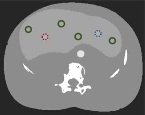
ROIs for TAC and perfusion RMSE calculation. The ROI for the homogeneous and Gaussian tumors are marked in dotted red (left) and dotted blue (right) respectively and other circles show healthy liver tissue with green.

To consider the effects of noise, five different noise realizations were generated and reconstructed for all comparisons. Standard deviations over noise realizations were computed for each time point to place error bars on TAC estimate curves, their corresponding RMSE plots, and to the RMSE plots for the perfusion maps.

IV. Results

A. Regularization Investigation

PL was used to reconstruct the simulated images using various regularization parameters β swept linearly (in exponent) from 10^0.5 to 10⁴ at 10^0.5 increments. The regularization parameter that resulted in the lowest RMSE was chosen as the optimal setting. Across all time points β = 10^1.5 resulted in the best RMSE. This suggests an optimization for each time point is not strictly required for PL.

An illustration of the 2D (β_R, β_M) RoD optimization is shown for I₀ = 10³ and t = 21 (s) in Figure 7. Both the RMSE and a zoomed ROI of the reconstructed difference images are shown as a function of both regularization parameters. The best image quality in terms of RMSE has been achieved by setting β_R = 10 and β_M = 10. As shown in Figure 7(B), noise increases for lower β_R values while parameter values larger than 10^1.5 significantly blurred the difference image. Similarly, larger values of β_M decreases noise; however, values larger than 10³ discourage change so much that the difference images become zero. While this optimization was performed with an explicit 2D search the structure of the error in Figure 7(A) suggests (as observed in [21] that a directed 1D search could be applied).

Figure 7.

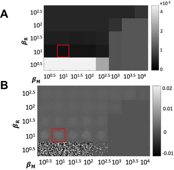
Results of regularization investigation for RoD with I₀ = 10³ and t = 21 s. (A) Regional RMSE (mm⁻¹) as a function of penalty coefficients β_R and β_M evaluated using a 10^0.5 interval. (B) A zoomed ROI showing difference reconstructions μ_Δ associated with each regularization parameter pair. The red box denotes the optimal β_R and β_M values.

Repeating the optimal parameter search for all time points, one finds a varying optimal regularization strength as a function of time. These optima are shown in Figure 8(A). Note that the optimal value of β_R is decreases for increasing contrast between tumor and healthy liver tissue. Similarly, we see the opposite relationship for β_M – increasing contrast between the tumor and healthy tissue corresponds to lower optimal β_M values. This suggests that traditional regularization works better for high contrast regions and prior-image-based regularization is more important in low contrast regions. A similar optimization was conducted for PIPLE the time-varying optima for this approach are shown in Figure 8(B). Note that the optimal value of β_R is decreases for increasing the contrast while β_P is lower for increased contrast between the tumor and surrounding healthy tissue (similar to RoD).

Figure 8.

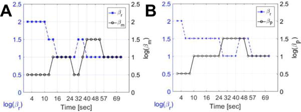
Optimal penalty coefficients, (A) for RoD, β_R and β_M, and (B) for PIPLE, β_R and β_P, as a function of time for incident fluence I₀ = 10³.

A. Incident Fluence Investigation

Figure 9(A) and 9(B) show the comparison of reconstructed images using FDK, PL, PIPLE and RoD reconstruction techniques near the splenic peak (t = 21 seconds) in the temporal series respectively for homogeneous and Gaussian tumors. The performance of all three methods deteriorated as the incident fluence decreased to I₀ = 5×10², however RoD performed better consistently. FDK had relatively poor visualization of the lesion at all but the highest fluence levels. The I₀ = 10³ represents a challenging case for all methods; however, RoD is able to perform significantly better than both PL and FDK. These qualitative assessments are echoed in the RMSE values shown in Figure 9(C) and 9(D). The rank ordering of methods is consistent across all fluence levels with RoD outperforming PL, PIPLE and FDK, and FDK performing worst. The error bars in Figure 9(C) and 9(D) for different noise realizations shows that the rank order performance has not changed and performance differences are greater than the error bars.

Figure 9.

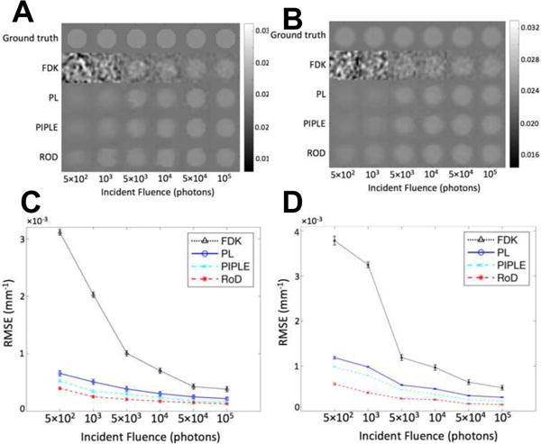
Comparison of reconstructions with incident fluence ranging from 5ran² to 10⁵ at t = 21 (s). (A) Homogeneous tumor ROI of the reconstructed volume using FDK, PL, PIPLE and RoD for different incident fluence values, and (B) Gaussian tumor ROI of the reconstructed volume using FDK, PL, PIPLE and RoD for different incident fluence values, (C) corresponding RMSE plots of FDK, PL, PIPLE and RoD for homogeneous tumor, and (D) corresponding RMSE plots of FDK, PL, PIPLE and RoD for Gaussian tumor.

B. Comparison of TACs and Perfusion Maps

Figure 10(A) and 10(B) show individual reconstruction of the homogeneous and Gaussian tumors ROIs across all time points using each reconstruction method for I₀ = 10³, as well as the corresponding ground truth images. Qualitative comparison of reconstructed images shows that RoD and PIPLE yielded better image quality across the entire range, even in low contrast regions. In contrast FDK exhibits strong noise across all points. PL performs better but appears to have increased blur as compared with RoD and PIPLE. TACs associated with these reconstructions are shown in Figure 10(C), (D) and (E) for the homogeneous, Gaussian tumor and healthy liver tissues, respectively. RMSE plots associated with these estimates are shown in Figure 10(F), (G) and (H). Stochastic fluctuations observed in the TACs are strongest for FDK and are mitigated by MBIR methods. The best results are found of RoD which has the lowest RMSE across all time points. This includes an improved RMSE over the other prior image method, PIPLE. Errors are generally higher in the tumor ROI (which was averaged over fewer voxels). Similarly, one might expect the healthy liver ROI to have lower RMSE since it is in a more homogeneous region.

Figure 10.

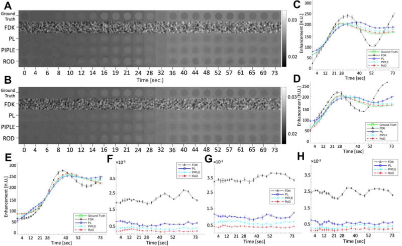
(A) Comparison of homogeneous tumor ROI and (B) Gaussian tumor ROI for FDK, PL, PIPLE and RoD reconstructions for incident fluence I₀ = 10³ and TAC estimates from FDK, PL, PIPLE and RoD reconstructions for incident fluence I₀ = 10³, (C) TAC estimates for the homogeneous tumor ROI, (D) TAC estimates for the Gaussian tumor ROI (E) TAC plot resulting from averages over healthy liver tissue ROIs. (F) RMSE plot for TAC shown in (C) and (G) RMSE plot for TAC shown in (D) and (H) RMSE plot for TAC shown in (E).

Figure 11(A) shows the calculated perfusion maps including HAP, HPP, PI and TTP maps for different reconstruction techniques at an incident fluence of I₀ = 10³. Reconstruction results are shown for the central slice, however similar results were achieved out of plane (suggesting cone-beam artifacts do not play a significant role). Consistent with previous results FDK exhibits increased noise as compared with other approaches. PL performs better but increased blue in the PI map reduces conspicuity of the tumor. Similarly, the tumor does not appear in the TTP map. PIPLE performs better than both FDK and PL, however the intensity of tumor region in the PI map is still lower than RoD and TTP map also shows a noisy appearance for the liver tissue. RoD outperforms the other methods with better tumor PI contrast and a conspicuous tumor apparent in the TTP map. PL and RoD appear to perform comparably for the HAP and HPP maps. RMSE comparisons for these perfusion maps are presented in Figure 11(B), (C) and (D) for the healthy liver, homogeneous and Gaussian tumor ROIs. Again, the quantitative results reinforce the qualitative observations with improved performance using RoD. The differences are greatest for PI and in the tumor ROI. Similar performance of PL, PIPLE and RoD in the tumor ROI is also noted.

Figure 11.

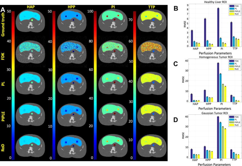
(A) HAP, HPP, PI and TTP maps for FDK, PL, PIPLE and RoD reconstruction methods compared to ground truth for incident Fluence I₀ = 10³. RMSE comparisons for the perfusion maps for (B) healthy liver, (C) homogeneous tumor and, (D) Gaussian tumor ROIs are also shown. The units for HAP and HPP is ml/min/100 ml and for TPP is seconds

V. DISCUSSION

In this paper, a novel scheme for acquiring and processing sequential CTP data was developed using the Reconstruction of Difference algorithm. In particular, an initial high-quality baseline reconstruction of the unenhanced anatomy was used to improve the image quality of subsequent reconstructions of low-exposure contrast-enhance CT data. Both RoD and PIPLE outperform traditional approaches by adding more information to the problem in the form of an additional regularization penalty that includes the prior image. It is interesting to note that RoD showed better performance than PIPLE, which suggests that the direct reconstruction of the perfusion enhancement is an advantage. That is, regularization of the parameters of interest (i.e., the contrast difference) allows for better perfusion estimates. The improved performance was demonstrated across a range of exposures for individual time-point reconstructions, for time-attenuation curve estimates, and in the computation of common perfusion metric maps.

The experimental conditions used a high-quality baseline (unenhanced) image volume acquired at a fluence of 10⁵ photons per detector element (which is a clinically relevant exposure in our experience). Using RoD suggests that this exposure could be dropped to 10³ photons and retain useful perfusion images instead of repeating the 10⁵ photon exposure over 20 times. In the low-exposure RoD case, the dose would be dominated by the initial baseline scan representing a substantial dose reduction. Naturally, this analysis is incomplete since readout noise and other effects are not taken into account. However, these preliminary results suggest the underlying methodology is a potentially powerful approach that can be applied in sequential data reconstruction like CT perfusion. Moreover, such methods may enable techniques like liver CTP which have not found widespread clinical use due to radiation dose concerns.

One practical challenge lies in RoD parameter optimization. While this investigation focused on optimal regularization with known truth, optimal prospective regularization design for prior-image methods is an ongoing research area [38], [39].

While the studies in this work suggest an opportunity for significant dose reduction, a number of simplifications were used in simulation physical and anatomical models. For example, beam hardening, scattered radiation, and readout noise effects were ignored in this work. However, all reconstruction algorithms must contend with these effects, and corrections tend to increase noise. In related work, we have successfully integrated beam hardening and scatter corrections into iterative reconstruction [40], [41] including cross-modality RoD where prior image CT and follow-up CBCT have different physical characteristics [42]. Thus, it is possible to include additional effects into all of these methods. While MBIR methods are an effective way to deal with increased noise, we would expect a decrease in performance of all methods with scatter and beam hardening, though the rank ordering of methods should remain the same.

The anatomical model used in this study was also simplified – e.g., a homogeneous liver without detailed vasculature. Such differences could have an impact on performance in clinical data (e.g. complicating the identification of regions of interest for the perfusion metric calculations). Thus, the limitations of these simulation studies must ultimately be addressed in ongoing and future work which seeks to perform similar comparisons in animal and human studies. Patient motion will be an important factor to consider in clinical data acquisitions. We have previously investigated deformable registration techniques and successfully integrated them into prior-image-based reconstruction [22]. Registration was found to be important for successful integration of prior information. Registration modifications have previously been embed in the RoD pipeline [23], though additional modifications specific to liver perfusion are likely needed. In particular, registration to very low exposure data will present challenges due to noise, and an alternating reconstruction and registration approach [22] may be needed to obtain good registration.

References

- 1.Miles KA, Lee TY, Goh V, et al. Current status and guidelines for the assessment of tumour vascular support with dynamic contrast-enhanced computed tomography. Eur Radiol. 2012;22(7):1430–1441. doi: 10.1007/s00330-012-2379-4. [DOI] [PubMed] [Google Scholar]
- 2.Bisdas S, Baghi M, Wagenblast J, et al. Differentiation of benign and malignant parotid tumors using deconvolution-based perfusion CT imaging: Feasibility of the method and initial results. Eur J Radiol. 2007;64(2):258–265. doi: 10.1016/j.ejrad.2007.02.032. [DOI] [PubMed] [Google Scholar]
- 3.Sahani DV, Kalva SP, Hamberg LM, et al. Assessing Tumor Perfusion and Treatment Response in Rectal Cancer with Multisection CT: Initial Observations. Radiology. 2005;234(3):785–792. doi: 10.1148/radiol.2343040286. [DOI] [PubMed] [Google Scholar]
- 4.Hashimoto K, Murakami T, Dono K, et al. Assessment of the severity of liver disease and fibrotic change: The usefulness of hepatic CT perfusion imaging. Oncol Rep. 2006 Oct; [PubMed] [Google Scholar]
- 5.Kim SH, Kamaya A, Willmann JK. CT Perfusion of the Liver: Principles and Applications in Oncology. Radiology. 2014;272(2):322–44. doi: 10.1148/radiol.14130091. [DOI] [PMC free article] [PubMed] [Google Scholar]
- 6.Qian LJ, Zhuang ZG, Cheng YF, et al. Hemodynamic alterations in anterior segment of liver graft after right-lobe living-donor liver transplantation: computed tomography perfusion imaging findings. doi: 10.1007/s00261-009-9563-2. [DOI] [PubMed] [Google Scholar]
- 7.Weidekamm C, Cejna M, Kramer L, et al. Effects of TIPS on Liver Perfusion Measured by Dynamic CT. Am J Roentgenol. 2005 Feb;184(2):505–510. doi: 10.2214/ajr.184.2.01840505. [DOI] [PubMed] [Google Scholar]
- 8.Sahani DV, Holalkere N-S, Mueller PR, et al. Advanced hepatocellular carcinoma: CT perfusion of liver and tumor tissue–initial experience. Radiology. 2007;243(3):736–743. doi: 10.1148/radiol.2433052020. [DOI] [PubMed] [Google Scholar]
- 9.Ippolito D, Capraro C, Casiraghi A, et al. Quantitative assessment of tumour associated neovascularisation in patients with liver cirrhosis and hepatocellular carcinoma: role of dynamic-CT perfusion imaging. Eur Radiol. 2012 Apr;22(4):803–811. doi: 10.1007/s00330-011-2307-z. [DOI] [PubMed] [Google Scholar]
- 10.Ogul H, Kantarci M, Genc B, et al. Perfusion CT imaging of the liver: review of clinical applications. Diagnostic Interv Radiol. 2014;20:379–389. doi: 10.5152/dir.2014.13396. [DOI] [PMC free article] [PubMed] [Google Scholar]
- 11.Pandharipande PV, Krinsky GA, Rusinek H, et al. Perfusion Imaging of the Liver: Current Challenges and Future Goals. Radiology. 2005;234(3):661–673. doi: 10.1148/radiol.2343031362. [DOI] [PubMed] [Google Scholar]
- 12.Okada M, Kim T, Murakami T. Hepatocellular nodules in liver cirrhosis: State of the art CT evaluation (perfusion CT/volume helical shuttle scan/dual-energy CT, etc) Abdom Imaging. 2011;36(3):273–281. doi: 10.1007/s00261-011-9684-2. [DOI] [PubMed] [Google Scholar]
- 13.Chen M-L, Zeng Q-Y, Huo J-W, et al. Assessment of the hepatic microvascular changes in liver cirrhosis by perfusion computed tomography. World J Gastroenterol. 2009 Jul;15(28):3532–7. doi: 10.3748/wjg.15.3532. [DOI] [PMC free article] [PubMed] [Google Scholar]
- 14.Li H, Sun C, Xu Z, et al. Low-dose whole organ CT perfusion of the pancreas: preliminary study. Abdom Imaging. 2014 Feb;39(1):40–47. doi: 10.1007/s00261-013-0045-1. [DOI] [PubMed] [Google Scholar]
- 15.Murase K, Nanjo T, Ii S, et al. Effect of x-ray tube current on the accuracy of cerebral perfusion parameters obtained by CT perfusion studies. Phys Med Biol. 2005 Nov;50(21):5019–5029. doi: 10.1088/0031-9155/50/21/005. [DOI] [PubMed] [Google Scholar]
- 16.Prakash P, Kalra MK, Kambadakone AK, et al. Reducing abdominal CT radiation dose with adaptive statistical iterative reconstruction technique. Invest Radiol. 2010;45(4):202–210. doi: 10.1097/RLI.ob013e3181dzfeec. [DOI] [PubMed] [Google Scholar]
- 17.Hara AK, Paden RG, Silva AC, et al. Iterative reconstruction technique for reducing body radiation dose at CT: feasibility study. AJR Am J Roentgenol. 2009 Sep;193(3):764–71. doi: 10.2214/AJR.09.2397. [DOI] [PubMed] [Google Scholar]
- 18.Negi N, Yoshikawa T, Ohno Y, et al. Hepatic CT perfusion measurements: A feasibility study for radiation dose reduction using new image reconstruction method. Eur J Radiol. 2012;81(11):3048–3054. doi: 10.1016/j.ejrad.2012.04.024. [DOI] [PubMed] [Google Scholar]
- 19.Chen G-H, Tang J, Leng S. Prior image constrained compressed sensing (PICCS): a method to accurately reconstruct dynamic CT images from highly undersampled projection data sets. Med Phys. 2008;35(2):660–663. doi: 10.1118/1.2836423. [DOI] [PMC free article] [PubMed] [Google Scholar]
- 20.Nett BE, Brauweiler R, Kalender W, et al. Perfusion measurements by micro-CT using Prior Image Constrained Compressed Sensing (PICCS): Initial Phantom Results. doi: 10.1088/0031-9155/55/8/014. [DOI] [PMC free article] [PubMed] [Google Scholar]
- 21.Stayman JW, Dang H, Ding Y, et al. PIRPLE: a penalized-likelihood framework for incorporation of prior images in CT reconstruction. Phys Med Biol. 2013;58(21):7563. doi: 10.1088/0031-9155/58/21/7563. [DOI] [PMC free article] [PubMed] [Google Scholar]
- 22.Dang H, Wang AS, Sussman MS, et al. dPIRPLE: a joint estimation framework for deformable registration and penalized-likelihood CT image reconstruction using prior images. Phys Med Biol. 2014 Sep;59(17):4799–826. doi: 10.1088/0031-9155/59/17/4799. [DOI] [PMC free article] [PubMed] [Google Scholar]
- 23.Pourmorteza A, Dang H, Siewerdsen JH, et al. Reconstruction of difference in sequential CT studies using penalized likelihood estimation. Phys Med Biol. 2016 Mar;61(5):1986–2002. doi: 10.1088/0031-9155/61/5/1986. [DOI] [PMC free article] [PubMed] [Google Scholar]
- 24.Seyyedi S, Liapi E, Lasser T, et al. Evaluation of Low-Dose CT Perfusion for the Liver using Reconstruction of Difference. Fully 3D Image Recon in Radiology and Nuc Med. 2017 [Google Scholar]
- 25.Chen JH, Lin YC, Huang YS, et al. Induction of VX2 carcinoma in rabbit liver: comparison of two inoculation methods. Lab Anim. 2004 Jan;38(1):79–84. doi: 10.1258/00236770460734434. [DOI] [PubMed] [Google Scholar]
- 26.Buijs M, Vossen JA, Geschwind J-FH, et al. Quantitative proton MR spectroscopy as a biomarker of tumor necrosis in the rabbit VX2 liver tumor. J Vasc Interv Radiol. 2011 Aug;22(8):1175–80. doi: 10.1016/j.jvir.2011.03.016. [DOI] [PMC free article] [PubMed] [Google Scholar]
- 27.Unser M. Splines: a perfect fit for signal and image processing. IEEE Signal Process Mag. 1999;16(6):22–38. [Google Scholar]
- 28.D’Antò M, Cesarelli M, Bifulco P, et al. Study of different time Attenuation Curve processing in liver CT perfusion. Proc IEEE/EMBS Reg 8 Int Conf Inf Technol Appl Biomed ITAB, pp. 2010:0–3. [Google Scholar]
- 29.Long Y, Fessler JA, Balter JM. 3D forward and back-projection for X-ray CT using separable footprints. IEEE Trans Med Imaging. 2010;29(11):1839–1850. doi: 10.1109/TMI.2010.2050898. [DOI] [PMC free article] [PubMed] [Google Scholar]
- 30.Feldkamp LA. Practical cone-beam algorithm Sfrdr I _ f. 1984;1(6):612–619. [Google Scholar]
- 31.Gentile BK. The care and feeding of digital, pulse-shaping filters. RF Des. 2002;25(4):50–61. [Google Scholar]
- 32.Fessler JA. Statistical image reconstruction methods for transmission tomography. Med Image Process Anal. 2000;3:1–70. [Google Scholar]
- 33.Huber PJ. Robust Estimation of a Location Parameter. Ann Math Stat. 1964;35(1):73–101. [Google Scholar]
- 34.Erdogan H, Fessler JA. Monotonic algorithms for transmission tomography. IEEE Trans Med Imaging. 1999;18(9):801–814. doi: 10.1109/42.802758. [DOI] [PubMed] [Google Scholar]
- 35.Miles KA, Hayball MP, Dixon AK. Functional images of hepatic perfusion obtained with dynamic CT. Radiology. 1993;188(2):405–411. doi: 10.1148/radiology.188.2.8327686. [DOI] [PubMed] [Google Scholar]
- 36.Miles KA. Measurement of tissue perfusion by dynamic computed tomography. Br J Radiol. 1991;64(761):409–412. doi: 10.1259/0007-1285-64-761-409. [DOI] [PubMed] [Google Scholar]
- 37.Mayer TE, Hamann GF, Baranczyk J, et al. Dynamic CT perfusion imaging of acute stroke. AJNR Am J Neuroradiol. 2000;21(8):1441–9. [PMC free article] [PubMed] [Google Scholar]
- 38.Dang H, Siewerdsen JH, Stayman JW. Prospective regularization design in prior-image-based reconstruction. Phys Med Biol. 2015 Dec;60(24):9515–36. doi: 10.1088/0031-9155/60/24/9515. [DOI] [PMC free article] [PubMed] [Google Scholar]
- 39.Zhang H, Dang H, Gang GJ, et al. Prospective Regularization Analysis and Design for Prior-Image-Based Reconstruction of X-ray CT. Proceedings of the International Meeting on Fully Three-Dimensional Image Reconstruction in Radiology and Nuclear Medicine. 2017 p. accepted. [Google Scholar]
- 40.Sisniega A, Zbijewski W, Xu J, et al. High-fidelity artifact correction for cone-beam CT imaging of the brain. Phys Med Biol. 2015;60(4):1415–1439. doi: 10.1088/0031-9155/60/4/1415. [DOI] [PubMed] [Google Scholar]
- 41.Dang H, Stayman JW, Sisniega A, et al. Statistical reconstruction for cone-beam CT with a post-artifact-correction noise model: Application to high-quality head imaging. Phys Med Biol. 2015;60(16):6153–6175. doi: 10.1088/0031-9155/60/16/6153. [DOI] [PMC free article] [PubMed] [Google Scholar]
- 42.Zhang H, Gang GJ, Lee J, et al. Integration of prior CT into CBCT reconstruction for improved image quality via reconstruction of difference: first patient studies. 2017;1013211:1013211. no. March 2017. [Google Scholar]