Identification of relevant subtypes via preweighted sparse clustering

Abstract

Cluster analysis methods are used to identify homogeneous subgroups in a data set. In biomedical applications, one frequently applies cluster analysis in order to identify biologically interesting subgroups. In particular, one may wish to identify subgroups that are associated with a particular outcome of interest. Conventional clustering methods generally do not identify such subgroups, particularly when there are a large number of high-variance features in the data set. Conventional methods may identify clusters associated with these high-variance features when one wishes to obtain secondary clusters that are more interesting biologically or more strongly associated with a particular outcome of interest. A modification of sparse clustering can be used to identify such secondary clusters or clusters associated with an outcome of interest. This method correctly identifies such clusters of interest in several simulation scenarios. The method is also applied to a large prospective cohort study of temporomandibular disorders and a leukemia microarray data set.

1. Introduction

In biomedical applications, cluster analysis is frequently used to identify homogeneous subgroups in a data set that provide information about a biological process of interest. For example, in microarray studies of cancer, a common objective is to identify cancer subtypes that are predictive of the prognosis (survival time) of cancer patients (Bhattacharjee et al., 2001; Sorlie et al., 2001; van ’t Veer et al., 2002; Rosenwald et al., 2002; Lapointe et al., 2004; Bullinger et al., 2004). In studies of chronic pain conditions, such as fibromyalgia or temporomandibular disorders (TMD), one may wish to develop a more precise case definition for the condition of interest by identifying subgroups of patients with similar clinical characteristics (Jamison et al., 1988; Bruehl et al., 2002; Davis et al., 2003; Hastie et al., 2005). However, conventional clustering methods (such as k-means clustering and hierarchical clustering) may produce unsatisfactory results when applied to these types of problems.

Identification of relevant clusters in complex data sets presents several challenges. It is common that only a subset of the features will have different means with respect to the clusters. This is particularly true in genetic studies, where the majority of the genes are not associated with the outcome of interest. Moreover, it is possible that some other subset of the features form clusters that are not associated with the outcome of interest. In genetic studies, given that genes work in pathways, genes in the same pathway are likely to form clusters even if the pathway is not associated with the biological outcome of interest.

As a motivating example, consider the artificial data set represented in Fig. 1. This depicts a standard clustering scenario in which we are seeking to cluster n observations based on p measured features, where the data is in the form of a p × n matrix. We see that two sets of clusters exist in this data: a set of clusters where the observations differ with respect to features 1–50, and a separate set of clusters where observations differ with respect to features 51–250. Also, note that the difference between the cluster means is much greater for the clusters formed by features 51–250 than it is for the clusters formed by features 1–50. Thus, when conventional clustering methods are applied to this data set, they will most likely identify the clusters corresponding to features 51–250. We define these clusters to be primary clusters, as they are most likely to be identified by conventional clustering methods. However, if observations 1–100 are controls and observations 101–200 are cases, then we would be interested in the clusters corresponding to features 1–50, which would not be identified by most existing clustering methods. Such a cluster that differs with respect to different features than the primary clusters (and hence will not be identified by most conventional clusters methods that identify the primary clusters) will be referred to as a secondary cluster. See Nowak and Tibshirani (2008) for a more detailed discussion of this problem.

Fig. 1.

Artificial data set illustrating the limitations of conventional clustering methods. Suppose observations 1–100 are controls and observations 101–200 are cases. In this situation, one would be interested in the clusters formed by features 1–50, but most existing clustering methods would identify the clusters formed by features 51–250 (and hence does not identify the cluster formed by features 1–50).

Note that labeling one set of clusters as “primary” and other sets of clusters as “secondary” or “tertiary” is done for convenience and that these labels are somewhat arbitrary. For a given data set, one may obtain different “primary clusters” depending on the clustering method and distance metric used (among other possible factors). Also, there may be some overlap between the features that differ with respect to the primary clusters and the features that differ with respect to the secondary clusters. However, the list of features that differ with respect to the primary and secondary clusters should not be identical. (If they differed with respect to exactly the same set of features, one could identify the “secondary cluster” by simply increasing the number of clusters k. Specialized methods are only needed when there are features that differ with respect to the secondary clusters but not the primary clusters.)

A number of methods exist for clustering data sets when the clusters differ with respect to only a subset of the features (Ghosh and Chinnaiyan, 2002; Friedman and Meulman, 2004; Bair and Tibshirani, 2004; Raftery and Dean, 2006; Pan and Shen, 2007; Koestler et al., 2010; Witten and Tibshirani, 2010). In particular, the method of Nowak and Tibshirani (2008) is designed specifically for the situation described in Fig. 1. However, many of these methods are computationally intensive, and their running times may be prohibitive when applied to high-dimensional data sets. More importantly, with the exception of the method of Nowak and Tibshirani (2008), these methods only produce a single set of clusters. If the clusters identified by the method are not related to the biological outcome of interest, there is no simple way to identify the more relevant secondary clusters. Also, these methods generally do not consider an outcome variable or any other biological information that could help identify the clusters of interest. In other words, if these methods are applied to a data set similar to Fig. 1, they are likely to produce clusters that are not related to the outcome of interest.

The problem of identifying clusters associated with an outcome variable has also not been studied extensively (Bair, 2013). In many situations, there is an outcome variable that is a “noisy surrogate” (Bair and Tibshirani, 2004; Bair et al., 2006) for the true clusters. For example, in genetic studies of cancer, it is believed that there are underlying subtypes of cancer with different genetic aberrations, and some subtypes may be more responsive to treatment (Rosenwald et al., 2002; Bullinger et al., 2004; Bair and Tibshirani, 2004). These subtypes cannot be observed directly, but a surrogate variable such as the patient’s survival time may be available. In other words, the outcome variable provides some information about the clusters of interest, but the true cluster assignments are still unknown for all observations. An artificial example of this situation is shown in Fig. 2. In this example, the mean of the outcome variable for observations in cluster 2 is higher than the mean of the outcome variable for observations in cluster 1. However, there is considerable overlap in the distributions. Thus, higher values of the outcome variable increase the likelihood that an observation belongs to cluster 2, but any classifier that attempts to predict the cluster based on the outcome variable will have a high error rate.

Fig. 2.

Artificial example of a situation where the outcome variable is a “noisy surrogate” for the true clusters. In this artificial example, the density functions of the outcome variable for observations in each of two clusters are shown above. Observations in cluster 2 are more likely to have higher values of the outcome variable than observations in cluster 1, but there is considerable overlap between the two groups. Thus, classifying observations to clusters based solely on the outcome variable will result in a high misclassification error rate.

We propose a novel clustering method that is applicable in situations where one wishes to identify secondary clusters associated with an outcome of interest, such as the scenario illustrated in Fig. 1. It is based on a modification of the “sparse clustering” algorithm of Witten and Tibshirani (2010), which we call preweighted sparse clustering. It can be applied both to the general problem of identifying secondary clusters in data sets and to the special case where one wishes to identify clusters associated with an outcome variable. We will show that our proposed method produces more accurate results than competing methods in several simulated data sets and apply it to real-world studies of chronic pain and cancer.

2. Methods

This section will begin by briefly describing several existing methods for identifying clusters associated with a biological process of interest. We will then describe our proposed method as well as the simulated and real data sets to which the proposed method will be applied.

2.1. Related clustering methods

2.1.1. Sparse clustering

Suppose that we wish to cluster the p × n data matrix X, where p is the number of features and n is the number of observations. Assume that the clusters only differ with respect to some subset of the features. Witten and Tibshirani (2010) propose a method called “sparse clustering” to solve this problem. A brief description of the sparse clustering method is as follows: Let d_i,j,j′ be any dissimilarity measure between observations j and j′ with respect to feature i. (Throughout the remainder of this discussion, we will assume that d_i,j,j′ = (X_ij − X_ij′)² the Euclidean distance between X_ij and X_ij′.) Then Witten and Tibshirani (2010) propose to identify clusters C₁, C₂, … , C_K and weights w₁, w₂, … , w_p that maximize the weighted between-cluster sum of squares

$$\sum _{i=1}^p{w}_i\left(\frac{1}{n}\sum _{j=1}^n\sum _{j^{\prime }=1}^n{d}_{i,j,j^{\prime }}-\sum _{k=1}^K\frac{1}{n_k}\sum _{j,j^{\prime }\in C_k}{d}_{i,j,j^{\prime }}\right),$$ (1)

subject to the constraints ${\sum }_i{w}_i^2=1$,Σ_i|w_i| < s, and w_i ≥ 0 for all i, where s is a tuning parameter and n_k is the number of elements in cluster k. Note that the Σ_i|w_i| < s constraint forces some of the weights to 0 for sufficiently small values of s, resulting in clusters that are based on only a subset of the features (hence the term “sparse clustering”). This is similar to the constraint used in lasso regression (Tibshirani, 1996) to produce a sparse set of predictor variables. To maximize (1), Witten and Tibshirani (2010) use the following algorithm:

1. Initialize the weights as $w_1=w_2=\cdots =w_p=1/\sqrt{p}$.

2. Fix the w_i’s and identify C₁, C₂, … , C_K to maximize (1). This can be done by applying the standard k-means clustering method to the n × n dissimilarity matrix where the (j, j′) element is Σ_iw_id_i,j,j′.

3. Fix the C_i’s and identify w₁, w₂, … , w_p to maximize (1) subject to the constraints that ${\sum }_i{w}_i^2=1$ and Σ_i|w_i| < s. See Witten and Tibshirani (2010) for a description of how the optimal w_i’s are calculated.

4. Repeat steps 2 and 3 until convergence.

This procedure requires a user to choose the number of clusters k and the tuning parameter s. We will not discuss methods for choosing these parameters; see Witten and Tibshirani (2010) for an algorithm for choosing s, and see Tibshirani et al. (2001), Sugar and James (2003), or Tibshirani and Walther (2005) for several possible methods for choosing k.

Although this method correctly identifies clusters of interest in many situations, it tends to identify clusters that are dominated by highly correlated features with high variance, which may not be interesting biologically. It also does not consider the values of any outcome variables that may exist. Thus, in the situation illustrated in Fig. 1, there is no guarantee that the clusters identified by this method will be associated with the outcome of interest.

2.1.2. Complementary clustering

Methods have been developed to identify secondary clusters of interest that may be obscured by “primary” clusters consisting of large numbers of high variance features (such as the situation illustrated in Fig. 1). Nowak and Tibshirani (2008) proposed a method for uncovering such clusters, called complementary hierarchical clustering. Again assume that we wish to cluster the p × n data matrix X. The first step of this method performs traditional hierarchical clustering on X. This set of hierarchical clusters is used to generate a new matrix X′ that is defined to be the expected value of the residuals when each row of X is regressed on the group labels when the hierarchical clustering tree is cut at a given height. The expected value is taken over all possible cuts. This has the effect of removing high variance features that may be obscuring secondary clusters. Traditional hierarchical clustering is then performed on this modified matrix X′, yielding secondary clusters. Witten and Tibshirani (2010) proposed a modification of this procedure (called “sparse complementary clustering”) using a variant of the methodology described in Section 2.1.1.

One significant limitation of these methods is the fact that they are only applicable to hierarchical clustering. To our knowledge there are currently no published methods for identifying secondary clusters based on partitional clustering methods such as k-means clustering.

2.1.3. Semi-supervised clustering methods

The situation where the observed outcome variable is a noisy surrogate variable for underlying clusters is very common in real-world problems. However, there are relatively few clustering methods that are applicable for this type of problem (Bair, 2013). Bair and Tibshirani (2004) proposed a method that they called “supervised clustering”. Supervised clustering performs conventional k-means clustering or hierarchical clustering using only a subset of the features. The features are selected by identifying a fixed number of features that have the strongest univariate association with the outcome variable. For example, if the outcome is dichotomous, one would calculate a t-statistic for each feature to test the null hypothesis of no association between the feature and the outcome and then perform clustering using only the features with the largest (absolute) t-statistics. Koestler et al. (2010) proposed a method called “semi-supervised recursively partitioned mixture models” (or “semi-supervised RPMM”). This method is similar to the supervised clustering method of Bair and Tibshirani (2004) in that one first calculates a score for each feature (such a t-statistic) that measures the association between that feature and the outcome and then performs clustering using only the features with the largest univariate scores. The difference between semi-supervised RPMM and supervised clustering is that semi-supervised RPMM applies the RPMM algorithm of Houseman et al. (2008) to the surviving features rather than a more conventional k-means or hierarchical clustering model.

These methods have successfully identified clinically relevant subtypes of cancer in many different studies (Bair and Tibshirani, 2004; Bullinger et al., 2004; Chinnaiyan et al., 2008; Koestler et al., 2010). However, these methods have significant limitations. In particular, both supervised clustering and semi-supervised RPMM require a user to choose the number of features that are used to form the clusters, and the results of these methods can depend heavily on the number of “significant” features selected. Moreover, it is very unlikely that these methods will successfully identify the truly significant features that define the clusters while excluding irrelevant features.

2.2. Preweighted sparse clustering

To overcome the limitations of these methods, we propose the following modification of sparse clustering, which we call preweighted sparse clustering. The preweighted sparse clustering algorithm is described below:

1. Run the sparse clustering algorithm, as described previously.

2. For each feature, calculate the F-statistic, F_i, (and associated p-value q_i) for testing the null hypothesis that the mean value of the feature i does not vary across the clusters.

3. For each feature i, define:

   $$w_i=\{\begin{array}{ll}1/\sqrt{m}\hfill & \text{if}{q}_i\ge \alpha \hfill \\ 0\hfill & \text{otherwise},\hfill \end{array}$$

   where m is the number of q_i’s such q_i ≥ α.

4. Run the sparse clustering algorithm using these w_i’s (beginning with step 2) and continuing until convergence.

In other words, the preweighted sparse clustering algorithm first performs conventional sparse clustering. It then identifies features whose mean values differ across the clusters. Then the sparse clustering algorithm is run a second time, but rather than giving equal weights to all features as in the first step, this preweighted version of sparse clustering assigns a weight of 0 to all features that differed across the first set of clusters. The motivation is that this procedure will identify secondary clusters that would otherwise be obscured by clusters that have a larger dissimilarity measure (such as the situation illustrated in Fig. 1).

This procedure requires one to choose a p-value threshold α for deciding which features should be given nonzero weight. An obvious choice is α = 0.05/p, where p is the number of features. However, the user may choose a less or more stringent cutoff depending on the sample size and other considerations. (Note that the F-statistic was calculated after clustering was performed, so the test statistic need not have an F distribution under the null hypothesis of no mean difference between clusters. Thus, these p-values should not be used to conclude that a given feature is associated with the clusters; this procedure is used only as a filtering technique. Indeed, the problem of identifying the features that differ with respect to clusters is a difficult problem that is beyond the scope of the present study.) Also note that this procedure may be repeated multiple times if one wishes to identify tertiary or higher order clusters.

If desired, one may normalize the data such that all features have mean 0 and standard deviation 1 before applying the methodology. This is recommended for most applications to avoid giving undue weight to features with higher variance. Unless otherwise noted, the data will be normalized before applying preweighted sparse clustering in all subsequent examples.

2.3. Supervised sparse clustering

The preweighted sparse clustering algorithm described above is an unsupervised method, since it does not require or use an outcome variable. If an outcome variable is available and the objective is to identify clusters associated with the outcome variable, one may use the following variant of preweighted sparse clustering to incorporate such data, which we call supervised sparse clustering. The supervised sparse clustering procedure is described below:

1. Let T_i be a measure of the strength of the association between the ith feature and the outcome variable. (If the outcome variable is dichotomous, T_i could be a t-statistic, or if the outcome variable is a survival time, T_i could be a univariate Cox score.) Let T₍₁₎, T₍₂₎, … , T_(p) denote the order statistics of the T_i’s.

2. Run the sparse clustering algorithm with initial weights w₁, w₂, … , w_p, where

   $$w_j=\{\begin{array}{ll}1/\sqrt{m}\hfill & \text{if}\mid T_i\mid \ge \mid T_{(p-m+1)}\mid \hfill \\ 0\hfill & \text{otherwise.}\hfill \end{array}$$

3. Run the standard sparse clustering algorithm using these w_i’s (beginning with step 2 and continuing until convergence.

In other words, supervised sparse clustering chooses the initial weights for the sparse clustering algorithm by giving nonzero weights to the features that are most strongly associated with the outcome variable. Note that no initial clustering step is required. This is similar to the semi-supervised clustering method of Bair and Tibshirani (2004) and the semi-supervised RPMM method of Koestler et al. (2010).

The supervised sparse clustering procedure requires the choice of a tuning parameter m, which is the number of features to be given nonzero weight in the first step. Our experience suggests that the procedure tends to give very similar results for a wide variety of different values of m; therefore, optimizing the procedure with respect to this tuning parameter is unnecessary. As a default we suggest $m=\sqrt{p}$, where p is the number of features. We will use this default throughout this manuscript unless otherwise noted.

2.4. Simulated data sets

A series of simulations were performed to evaluate the performance of our proposed methods and to compare them to the results of existing methods. Several additional simulation studies are described in Section S1 in the Supplementary materials.

2.4.1. A motivating example

A single 50 × 100 data set was generated as follows:

$$X_{ij}=\{\begin{array}{ll}6+{\epsilon }_{ij}\hfill & \text{if}i\le 10,j\le 50\hfill \\ -6+{\epsilon }_{ij}\hfill & \text{if}i\le 10,j>50\hfill \\ 9+{\epsilon }_{ij}\hfill & \text{if}11\le i\le 20,j\le 50,\text{and}j\text{odd}\hfill \\ 3+{\epsilon }_{ij}\hfill & \text{if}11\le i\le 20,j\le 50,\text{and}j\text{even}\hfill \\ -3+{\epsilon }_{ij}\hfill & \text{if}11\le i\le 20,j\le 50,\text{and}j\text{odd}\hfill \\ -9+{\epsilon }_{ij}\hfill & \text{if}11\le i\le 20,j\le 50,\text{and}j\text{even}\hfill \\ 3+{\epsilon }_{ij}\hfill & \text{if}i\le 21\le 30,j\text{odd}\hfill \\ -3+{\epsilon }_{ij}\hfill & \text{if}i\le 21\le 30,j\text{even}\hfill \\ {\epsilon }_{ij}\hfill & \text{if}i>30.\hfill \end{array}$$ (2)

In this data set, the primary clusters are defined by rows 1–20 and the secondary clusters are defined by rows 11–30. The objective of this simulation is to determine if preweighted sparse clustering can identify both the primary and secondary clusters and assign nonzero weight to the appropriate features.

2.4.2. Preweighted sparse clustering

We generated a series of simulated data sets to evaluate the performance of preweighted sparse clustering and compare it to the complementary hierarchical clustering method of Nowak and Tibshirani (2008) and the complementary hierarchical sparse clustering method of Witten and Tibshirani (2010). We generated simulated data sets similar to the simulated data sets in Nowak and Tibshirani (2008), who generated a series of p × 12 data matrices as follows:

$$X_{ij}=\{\begin{array}{ll}a+{\epsilon }_{ij}\hfill & \text{if}i\le p_e,j\le n_a\hfill \\ -a+{\epsilon }_{ij}\hfill & \text{if}i\le p_e,j>n_a\hfill \\ {\epsilon }_{ij}\hfill & \text{if}{p}_e<i<p-p_e\hfill \\ b+{\epsilon }_{ij}\hfill & \text{if}i\ge p-p_e,j\text{odd}\hfill \\ -b+{\epsilon }_{ij}\hfill & \text{if}i\ge p-p_e,j\text{even.}\hfill \end{array}$$ (3)

Here, the ε_ij’s are iid normal random variables with mean 0 and standard deviation σ. See Fig. 3 for a graphical illustration of this data set. The expectation is that the first p_e rows (i.e., “Effect 1”) will be identified as the “primary clusters” and the final p_e rows (i.e., “Effect 2”) will be identified as the “secondary clusters”.

Fig. 3.

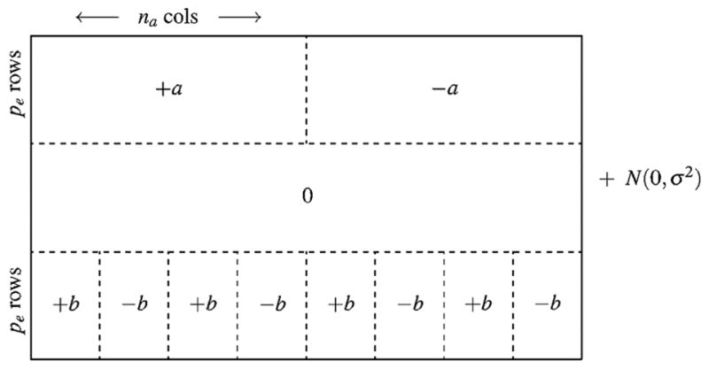
Schematic illustration of the simulated data set. The top p_e rows correspond to the “primary clusters” (i.e., “Effect 1”) and the bottom p_e rows correspond to the “secondary clusters” (i.e., “Effect 2”).

Source: Reprinted with permission from Nowak and Tibshirani (2008).

We considered four simulation scenarios (similar to the four simulation scenarios considered in Nowak and Tibshirani (2008). We let a = 6 in all four scenarios. Unless otherwise specified, we also let b = 3, σ = 1, and n_a = 6 for each simulation scenario. For the first three scenarios, 1000 matrices were generated with p = 50 and p_e = 20. In the first scenario, we varied the value of b. In the second scenario, we varied the value of σ, and in the third scenario, we varied n_a. In the final scenario, we generated 100 matrices with p = 2000 and varied the value of p_e. (The first three scenarios are identical to the simulations of Nowak and Tibshirani (2008); the final scenario was modified slightly for computational reasons.)

Preweighted sparse clustering, complementary hierarchical clustering, and complementary hierarchical sparse clustering were applied to each simulated data set. The number of clusters was fixed to be k = 2 for all methods. Both hierarchical clustering methods used average linkage. For complementary hierarchical clustering, two distance metrics were considered. The first metric defined the distance between observations j and j′ was defined to be 1 − corr(x_·j, x_·j′), which is the same distance metric used by Nowak and Tibshirani (2008). The second distance metric was Euclidean distance. Complementary hierarchical sparse clustering only used Euclidean distance, since the correlation distance metric is not implemented for that procedure.

Each set of clusters identified by each method was compared to the true cluster labels for both Effect 1 and Effect 2. The number of simulations for which each method correctly identified Effect 1 and/or Effect 2 was recorded. The results of a clustering procedure were considered to be incorrect if one or more observations were assigned to the incorrect cluster.

2.4.3. Supervised sparse clustering

In an additional set of simulations, we generated a series of 1000 simulated data sets to test the supervised sparse clustering algorithm. Specifically, we generated 1000 5000 × 200 data matrices X where

$$\begin{gathered} X_{ij}= \\ \{\begin{array}{ll}1+{\epsilon }_{ij}\hfill & \text{if}i\le 50,j\le 100\hfill \\ 2+{\epsilon }_{ij}\hfill & \text{if}i\le 50,j>100\hfill \\ 2I(u_{ij}<0.4)+{\epsilon }_{ij}\hfill & \text{if}51\le i\le 100\hfill \\ 0.5I(u_{ij}<0.7)+{\epsilon }_{ij}\hfill & \text{if}101\le i\le 200\hfill \\ 1.5I(u_{ij}<0.3)+{\epsilon }_{ij}\hfill & \text{if}201\le i\le 300\hfill \\ {\epsilon }_{ij}\hfill & \text{if}i>300.\hfill \end{array} \end{gathered}$$

Here I(x) is an indicator function, and the u_ij’s are iid uniform random variables on (0, 1). The ε_ij’s are iid standard normal, as before. We also defined the binary outcome variable y as follows:

$$y_i=\{\begin{array}{ll}0+I(u_i<0.3)\hfill & \text{if}1\le i\le 100\hfill \\ 1-I(u_i<0.3)\hfill & \text{if}101\le i\le 200.\hfill \end{array}$$

(In the above, once again I(x) is an indicator function and the u_i’s are iid uniform random variables on (0, 1).) This simulation is similar to the scenario illustrated in Fig. 1. We assume that the first 50 features are the biologically relevant features of interest. In other words, a clustering algorithm that achieves perfect accuracy should assign observations 1–100 to one cluster and observations 101–200 to a separate cluster. Features 51–100, 101–200, and 201–300 also form clusters, but these clusters are not related to the biological outcome of interest. The outcome variable y also observed is a “noisy surrogate” for the true clusters. This y is related to the true clusters, but 30% of the y_i’s are misclassified. This is consistent with what we might expect to observe in a study of chronic pain, where the only observed outcome variable is a patient’s subjective pain report, which is not always a reliable indicator of case status.

The objective of this simulation is to determine if supervised sparse clustering can correctly identify the clusters that are associated with the y_i’s, as opposed to the other sets of clusters that are not related to the outcome. Supervised sparse clustering was applied to each of the 1000 simulated data sets. Three other methods were also considered, namely conventional sparse k-means clustering, the semi-supervised k-means clustering method of Bair and Tibshirani (2004), and conventional k-means clustering on the first three principal components of the data set. The number of clusters was fixed to be k = 2 under all methods. We also attempted to apply the semi-supervised RPMM method of Koestler et al. (2010) to these simulated data sets, but in each case the procedure returned a singleton cluster. The number of observations assigned to the incorrect cluster was recorded for each method for each simulation.

2.5. OPPERA data

Orofacial Pain: Prospective Evaluation and Risk Assessment (OPPERA) is a prospective cohort study designed to identify risk factors for temporomandibular disorders (TMD). OPPERA recruited a total of 3258 TMD-free study subjects at four U.S. study sites from May 2006 to November 2008. Numerous putative risk factors for first-onset TMD were evaluated at the time of enrollment, and after enrollment each participant completed a quarterly follow up questionnaire assessing TMD pain symptoms. Those reporting symptoms were invited for a follow up exam to determine if they had developed first-onset TMD. The median follow up period was 2.8 years, and a total of 260 participants developed TMD over the course of the study. For a more detailed description of the OPPERA study, see Maixner et al. (2011a), Slade et al. (2011) or Bair et al. (2013).

We applied our clustering algorithms to the baseline data collected in OPPERA. Specifically, we included all of the measures of experimental pain sensitivity, psychological distress, and autonomic function. See Greenspan et al. (2011), Fillingim et al. (2011), and Maixner et al. (2011b) for a more detailed description of these variables. A total of 116 predictor variables were used, including 33 measures of experimental pain sensitivity, 39 measures of psychological distress, and 44 measures of autonomic function. The primary outcome of interest is time until the development of first-onset TMD. Since some participants did not develop first-onset TMD before the end of the follow up period, the outcome was treated as a censored survival time.

In our analysis of the OPPERA data, we applied the preweighted sparse clustering algorithm as outlined in Section 2.2. Conventional sparse clustering was applied to the data set (also with k = 2), after which the features that showed strongest mean differences across the clusters were given a weight of 0 when the preweighted version of sparse clustering was applied. The preweighted version was then applied for a second time in the same manner to identify tertiary clusters. All features were normalized to have mean 0 and standard deviation 1 prior to performing the clustering. The association between both the primary clusters and secondary clusters and the time until first-onset TMD was evaluated using Cox proportional hazards models. Complementary hierarchical clustering was also applied to both data sets for comparison. Complementary sparse hierarchical clustering was not considered for computational reasons.

We also applied our supervised sparse clustering, sparse clustering, preweighted sparse clustering, semi-supervised clustering, and clustering on the (first five) principal component scores to the OPPERA data. We let k = 2 for each method. To verify that associations between clusters and first-onset TMD are not the results of overfitting, the data set was randomly partitioned into a training set and a test set with an equal number of cases of first-onset TMD in both partitions. To identify the “most significant” predictors of first-onset TMD before applying supervised sparse clustering and semi-supervised clustering, the association between each feature and first-onset TMD was evaluated by calculating the univariate Cox score for each feature. See Beer et al. (2002) or Bair and Tibshirani (2004) for more information. Each clustering method was applied to the training data and a lasso model (Tibshirani, 1996; Friedman et al., 2010) was fit to the training data to predict the resulting clusters. This lasso model was then used to predict the clusters on the test data. The association between the predicted clusters and first-onset TMD was evaluated by fitting a Cox proportional hazards model on the test data. Note that the test data was not used to identify the features associated with first-onset TMD nor to identify the initial clusters, so any association between the predicted clusters on the test data and first-onset TMD cannot be explained by overfitting.

2.6. Leukemia microarray data

We applied our supervised sparse clustering algorithm to the leukemia microarray data of Bullinger et al. (2004). This data set includes data for 116 subjects with acute myeloid leukemia. Gene expression data for 6283 genes are recorded for each subject, as well as survival times and outcomes. Survival times ranged from 0 to 1625 days, with an average time of 407.1 days. The objective was to identify genetic subtypes (i.e. clusters) using the gene expression data that could be used to predict the prognosis of leukemia patients.

We applied our supervised sparse clustering method to this data set as well conventional sparse clustering, preweighted sparse clustering, semi-supervised clustering, and clustering on the PCA scores. The number of clusters was taken to be 2 in all methods. Before applying any of the clustering methods, all features were normalized to have mean 0 and standard deviation 1 and the data were randomly partitioned into a training set and a test set, each of which consisted of 58 observations. Each clustering method was applied to the training data. To identify the “most significant” genes for supervised sparse clustering and semi-supervised clustering, the association between each gene and survival was evaluated by calculating the univariate Cox score for each gene. For each set of clusters, a nearest shrunken centroid model (Tibshirani et al., 2002) was fit to the clusters in the training data and then applied to the test data to predict cluster assignments on the test data. (As in the previous example, clusters were predicted on an independent test set to ensure that the results are not due to overfitting.) The association between the predicted clusters in the test set and survival was evaluated using Cox proportional hazards models for each clustering method.

3. Results

3.1. Simulated data sets

3.1.1. Motivating example

Preweighted sparse clustering correctly identified both the primary and secondary clusters in this example. The feature weights for the primary clusters as well as the initial and final feature weights for the secondary clusters are shown in Fig. 4. The procedure identifies the primary clusters correctly and assigns nonzero weight to the appropriate observations. Since preweighted sparse clustering initially assigns zero weight to features that are associated with the primary clusters and equal weight to features that are not associated with the primary clusters, this means that initially features 11–20 (which are associated with the secondary clusters) have a weight of zero and features 31–50 (which are not associated with the secondary clusters) have a nonzero weight. When the procedure terminates, however, features 11–20 have nonzero weight and features 31–50 have (effectively) zero weight.

Fig. 4.

This figure shows the feature weights for the primary clusters as well as the initial and final feature weights for the secondary clusters for the motivating example. Note that the procedure for identifying secondary clusters initially gives a weight of 0 to features 11–20 (since they are also associated with the primary clusters) and nonzero weight to features 31–50 (since they are not associated with the primary clusters). When the procedure terminates, however, features 11–20 have nonzero weight and features 30–50 have (effectively) zero weight.

This result is important because it demonstrates that preweighted sparse clustering and supervised sparse clustering can accurately identify clusters (and the features that define these clusters) even if the initial cluster weights give zero weight to some relevant features and nonzero weight to irrelevant features. Thus, it is not essential to choose an “optimal” set of initial weights since the procedure tends to correct itself. The implication is that these methods are robust to giving too many (or too few) features nonzero weight at the initial step. This is potentially an advantage of supervised sparse clustering compared to existing supervised clustering methods (Bair and Tibshirani, 2004; Koestler et al., 2010) that merely cluster on a subset of the features that are most strongly associated with the outcome. Once these methods choose a set of features to use for the clustering, that set of features is fixed, so the results may depend heavily on the features chosen (and a suboptimal choice of features may produce poor results). By contrast, supervised sparse clustering (and preweighted sparse clustering) tends to self-correct so that relevant features get nonzero weight (even if their initial weight was zero) and irrelevant features get zero weight (even if their initial weight was nonzero).

In practice it is often difficult to determine if a feature weight produced by sparse clustering is “significantly” different from 0. Thus, our procedures do not attempt to find an exhaustive list of all features associated with the clusters. (One may find a list of at least some features associated with the clusters by increasing the value of the tuning parameter s, but increasing s too much can cause features truly associated with the outcome to have zero weight.) This simulation demonstrates that preweighted sparse clustering tends to give nonzero weight to the correct features even if there is no simple way to determine which features have truly nonzero weight.

3.1.2. Preweighted sparse clustering

The results of the set of simulation scenarios are shown in Tables 1, 2, 3, and 4. Preweighted sparse clustering produced the best results in the first simulation scenario and generally performed the best in the second simulation scenario. Specifically, preweighted sparse clustering correctly identified both the primary and secondary clusters for small values of b in the first scenario and for large values of σ in the second scenario (although it appears to be slightly less likely to correctly identify the secondary clusters in the second scenario for σ ≥ 5). This indicates that preweighted sparse clustering may produce more accurate results than the competing methods when the signal to noise ratio is low (either because the mean difference in the two clusters is small or the amount of random noise is large). All three methods performed well in the third simulation scenario, with both complementary hierarchical methods performing perfectly. The results of the final simulation were mixed. Complementary hierarchical clustering never correctly identified both the primary and secondary clusters for small values of p_e whereas preweighted sparse clustering did identify both clusters in at least some simulations for all p_e > 4. However, complementary hierarchical clustering always correctly identified at least one of the two clusters, whereas preweighted sparse clustering sometimes identified neither cluster correctly. Complementary sparse hierarchical clustering performed the best on this simulation scenario, with near perfect accuracy even for small values of p_e.

Table 1.

Results of the first simulation when the values of b (the difference between the means of the secondary clusters) were varied. The clusters associated with the first p_e rows were defined to be “Effect 1”, and the clusters associated with the final p_e rows were defined to be “Effect 2”. “Effect 1/Effect 2” means that the primary clusters identified by the procedure correspond to Effect 1 and the secondary clusters correspond to Effect 2. “Effect 1/Neither” means that the primary clusters corresponded to Effect 1 but the secondary clusters corresponded to neither Effect 1 nor Effect 2. PSC=preweighted sparse clustering, CHC=complementary hierarchical clustering (using both correlation and Euclidean distance), CSHC=complementary sparse hierarchical clustering.

	b	Effect 1/Effect 2	Effect 2/Effect 1	Effect 1/Neither
PSC	0.5	419	0	581
	0.75	959	0	41
	1	998	0	2
	2	1000	0	0
	3	997	3	0
	6	512	488	0
CHC (corr.)	0.5	142	0	858
	0.75	591	0	409
	1	925	0	75
	2	1000	0	0
	3	1000	0	0
	6	488	512	0
CHC (Eucl.)	0.5	282	0	718
	0.75	826	0	174
	1	987	0	13
	2	1000	0	0
	3	1000	0	0
	6	488	512	0
CSHC	0.5	0	0	1000
	0.75	0	0	1000
	1	0	0	1000
	2	1000	0	0
	3	1000	0	0
	6	481	519	0

Table 2.

Results of the first simulation when the values of σ (the standard deviation of the simulated data) were varied. The clusters associated with the first p_e rows were defined to be “Effect 1”, and the clusters associated with the final p_e rows were defined to be “Effect 2”. “Effect 1/Effect 2” means that the primary clusters identified by the procedure correspond to Effect 1 and the secondary clusters correspond to Effect 2. “Effect 1/Neither” means that the primary clusters corresponded to Effect 1 but the secondary clusters corresponded to neither Effect 1 nor Effect 2. PSC=preweighted sparse clustering, CHC=complementary hierarchical clustering (using both correlation and Euclidean distance), CSHC=complementary sparse hierarchical clustering.

	σ	Effect 1/Effect 2	Effect 2/Effect 1	Effect 1/Neither	Effect 2/Neither	Neither/Neither
PSC	1	994	6	0	0	0
	2	1000	0	0	0	0
	2.5	1000	0	0	0	0
	3	993	0	7	0	0
	4	509	0	491	0	0
	5	18	0	982	0	0
	6	2	0	997	0	1
CHC (corr.)	1	1000	0	0	0	0
	2	985	0	15	0	0
	2.5	893	0	107	0	0
	3	568	0	432	0	0
	4	71	0	919	0	10
	5	8	0	887	0	105
	6	0	0	669	1	331
CHC (Eucl.)	1	1000	0	0	0	0
	2	995	0	5	0	0
	2.5	933	0	67	0	0
	3	648	0	352	0	0
	4	139	0	861	0	0
	5	28	0	971	0	1
	6	13	0	965	0	22
CSHC	1	1000	0	0	0	0
	2	1000	0	0	0	0
	2.5	981	0	19	0	0
	3	866	0	134	0	9
	4	328	0	672	0	1
	5	92	0	877	0	31
	6	17	0	811	0	172

Table 3.

Results of the first simulation when the values of n_a were varied (the number of observations in the first cluster for the primary clusters). The clusters associated with the first p_e rows were defined to be “Effect 1”, and the clusters associated with the final p_e rows were defined to be “Effect 2”. “Effect 1/Effect 2” means that the primary clusters identified by the procedure correspond to Effect 1 and the secondary clusters correspond to Effect 2. “Effect 1/Neither” means that the primary clusters corresponded to Effect 1 but the secondary clusters corresponded to neither Effect 1 nor Effect 2. PSC=preweighted sparse clustering, CHC=complementary hierarchical clustering (using both correlation and Euclidean distance), CSHC=complementary sparse hierarchical clustering.

	n	Effect 1/Effect 2	Effect 2/Effect 1
PSC	6	990	8
	8	993	7
	10	962	38
CHC (corr.)	6	1000	0
	8	1000	0
	10	1000	0
CHC (Eucl.)	6	1000	0
	8	1000	0
	10	1000	0
CSHC	6	1000	0
	8	1000	0
	10	1000	0

Table 4.

Results of the first simulation when the values of p_e (the number of observations in both the primary and secondary clusters) were varied. The clusters associated with the first p_e rows were defined to be “Effect 1”, and the clusters associated with the final p_e rows were defined to be “Effect 2”. “Effect 1/Effect 2” means that the primary clusters identified by the procedure correspond to Effect 1 and the secondary clusters correspond to Effect 2. “Effect 1/Neither” means that the primary clusters corresponded to Effect 1 but the secondary clusters corresponded to neither Effect 1 nor Effect 2. PSC=preweighted sparse clustering, CHC=complementary hierarchical clustering (using both correlation and Euclidean distance), CSHC=complementary sparse hierarchical clustering.

	pe	Effect 1/Effect 2	Effect 2/Effect 1	Effect 1/Neither	Effect 2/Neither	Neither/Neither
PSC	4	0	0	4	1	95
	8	8	4	31	14	43
	12	33	18	31	16	2
	16	64	23	9	4	0
	20	81	14	4	1	0
	24	83	16	1	0	0
CHC (corr.)	4	0	0	100	0	0
	8	0	0	100	0	0
	12	0	0	100	0	0
	16	79	0	21	0	0
	20	99	0	1	0	0
	24	100	0	0	0	0
CHC (Eucl.)	4	0	0	100	0	0
	8	0	0	100	0	0
	12	0	0	100	0	0
	16	4	0	96	0	0
	20	88	0	12	0	0
	24	100	0	0	0	0
CSHC	4	99	0	1	0	0
	8	100	0	0	0	0
	12	100	0	0	0	0
	16	100	0	0	0	0
	20	100	0	0	0	0
	24	100	0	0	0	0

3.1.3. Supervised sparse clustering

The mean number of misclassified observations (and associated standard errors) when each method is applied to the final set of simulations is shown in Table 5. Supervised sparse clustering produced the lowest error rate of all the methods, averaging 7.2 misclassifications. Semi-supervised clustering occasionally identified the correct clusters, but produced unsatisfactory results in many of the simulations. Conventional sparse clustering and k-means clustering on the principal component scores produced poor results in all the simulated data sets. Clustering on PCA scores often produced a singleton cluster, and semi-supervised RPMM returned a single cluster in each simulation.

Table 5.

Results of the second simulation study. The following methods were applied to the simulated data set described in Section 2.4: (1) supervised sparse clustering, (2) sparse clustering, (3) supervised clustering (Bair and Tibshirani, 2004), (4) k-means clustering on the top 3 principal component (PCA) scores. The mean number of misclassified observations (and associated standard errors) is shown for each method.

	Sup. sparse clust.	Sparse clust.	Sup. clust.	Clust. on PCA
Mean	7.2	94.5	11.3	95.1
SE	0.8	0.1	0.7	0.1

3.2. OPPERA data

We applied the preweighted sparse clustering method to the OPPERA data with k = 2. The weights for both the primary, secondary and tertiary clusters are shown in Fig. 5. Observe that the measures of autonomic function had the largest feature weights for the primary clusters, whereas the measures of psychological distress had the largest feature weights for the secondary clusters. Measures of thermal pain have the largest features weights for the tertiary clusters. Thus, the preweighted sparse clustering method revealed a biologically meaningful set of secondary and tertiary clusters that were not identified by the conventional sparse clustering algorithm.

Fig. 5.

Feature weights for the primary, secondary and tertiary clusters identified by the preweighted sparse clustering method. In the figure below, features 1–33 are measures of experimental pain sensitivity, features 34–72 are measures of psychological distress, and features 73–116 are measures of autonomic function. We see that the primary clusters differ from one another primarily with respect to measures of autonomic functions, the secondary clusters differ primarily with respect to measures of psychological distress and the tertiary clusters differ primarily with respect to measures of thermal pain.

The associations between the primary and secondary clusters identified by preweighted sparse clustering and hierarchical complementary clustering are shown in Table 6. The primary clusters identified by preweighted sparse clustering were not significantly associated with first-onset TMD (HR = 1.2, p = 0.09). However, the secondary clusters were associated with first-onset TMD (HR = 1.9, p = 6.5×10⁻⁷). Such a result suggests that clusters associated with an outcome of interest (first-onset TMD in this scenario) may be obscured by a set of clusters unrelated to the outcome of interest. The preweighted sparse clustering method was able to identify these obscured clusters. Neither the primary nor the secondary clusters identified by complementary hierarchical clustering were significantly associated with first-onset TMD.

Table 6.

The association between the incidence of first-onset TMD and the primary and secondary clusters identified by preweighted sparse clustering method and complementary hierarchical clustering on the OPPERA prospective cohort data. A Cox proportional hazards model evaluated the null hypothesis of no association between TMD incidence and the cluster assignments. The hazard ratio and associated p-values of each cluster are reported below.

		Hazard ratio	P-value
Preweighted sparse clustering	Primary cluster	1.2	0.09
	Secondary cluster	1.9	6.5 × 10−7
Complementary clustering	Primary cluster	1.0	0.98
	Secondary cluster	1.1	0.32

It is interesting to note that these results are consistent with previously published studies on the risk factors for first-onset TMD in the OPPERA study. As observed in Fig. 5, the primary clusters differed mainly with respect to measures of autonomic function whereas the secondary clusters differed mainly with respect to measures of psychological distress. Previous research found that the measures of autonomic function collected in OPPERA were not associated with first-onset TMD (Greenspan et al., 2013) whereas many psychological variables were strong predictors of first-onset TMD (Fillingim et al., 2013).

It is also interesting to compare these results with clusters identified by Bair et al. (2016). Bair et al. (2016) used a supervised clustering method to identify three clusters, one of which was associated with significantly greater risk of first-onset TMD than the other two clusters. Participants in this high-risk cluster had higher levels of pain sensitivity and psychological distress than participants in the other clusters. Our current findings suggest that rather than a single set of clusters associated with pain sensitivity and psychological distress, there may be a primary/secondary/tertiary hierarchy of clusters, with the secondary clusters (associated with psychological distress) driving the association between the clusters and first-onset TMD. Further research is needed to validate this hypothesis.

Finally, we applied supervised sparse clustering (as well as several other methods discussed earlier) to the OPPERA data. The results are shown in Table 7. The two supervised clustering methods identified clusters associated with first-onset TMD whereas the clusters identified by sparse clustering and clustering on the PCA scores were not associated with first-onset TMD. This suggests that clustering methods that consider an outcome variable may do a better job of identifying biologically relevant clusters than methods that do not consider this information. Also, the primary clusters identified by sparse clustering were not associated with first-onset TMD, while the secondary clusters identified by preweighted sparse clustering were associated with first-onset TMD. Note that Table 7 shows the results for predicted clusters on an independent test data set, so they cannot be attributed to overfitting.

Table 7.

Four different clustering methods were applied to the OPPERA prospective cohort training data. Each observation in the test data was assigned to a cluster by fitting a lasso model to predict the clusters on the training data and applying this model to the test data. The table below shows the association between each (predicted) cluster and first-onset TMD on the test data. For each method, a Cox proportional hazard model was performed to test the null hypothesis of no difference in survival between the two clusters. The hazard ratios and associated p-values are reported below.

	Hazard ratio	P-value
Supervised sparse clustering	2.2	5.8 × 10−5
Sparse clustering	1.1	0.69
Supervised clustering	3.1	3.0 × 10−8
Clustering on PCA scores	1.3	0.11
Preweighted sparse clustering (secondary cluster)	1.8	6.3 × 10−4

3.3. Leukemia microarray data

For each clustering method, the hazard ratio and associated p-values for the predicted test set clusters are shown in Table 8. Four of the methods produced clusters that were associated with patient survival, although the clusters produced by supervised sparse clustering were more strongly associated with survival than the clusters produced by the other methods. (The secondary clusters identified by preweighted sparse clustering were not associated with survival in this case.) This indicates that supervised sparse clustering can identify biologically meaningful and clinically relevant clusters in high-dimensional biological data sets. The fact that the predicted clusters were associated with survival on an independent test set suggests that this finding is not merely the result of overfitting.

Table 8.

The association between the predicted clusters for the test data and survival for the leukemia microarray data. For each method, a Cox proportional hazards model was used to test the null hypothesis of no difference in survival between the two predicted clusters. The hazard ratios and associated p-values are reported below.

	Hazard ratio	P-value
Supervised sparse clustering	3.4	6.0 × 10−4
Sparse clustering	2.2	0.042
Semi-supervised clustering	2.7	0.006
Clustering on PCA scores	2.4	0.024
Preweighted sparse clustering (secondary cluster)	1.9	0.08

4. Discussion

Cluster analysis is frequently used to identify subtypes in complex data sets. In many cases, the primary objective of the cluster analysis is to identify clusters that offer new insight into a biological question of interest or that can be used to more precisely phenotype (and hence diagnose and treat) a particular disease. However, in many cases, the clusters identified by conventional clustering methods are dominated by a subset of the features that are not interesting biologically or clinically.

Suppose one applies a conventional clustering method and identifies clusters that are not associated with the outcome of interest or are not interesting biologically or clinically. One may wish to identify secondary clusters that differ with respect to a different set of features that may be more interesting or useful. Despite the fact that this problem is very common in cluster analysis, relatively few methods have been proposed to identify clusters in these situations. As noted earlier, the idea of “complementary clustering” was first proposed by Nowak and Tibshirani (2008), and Witten and Tibshirani (2010) proposed an alternative method based on sparse clustering. However, these methods have several limitations. They can only be used with hierarchical clustering. To our knowledge, our proposed method is the first complementary clustering algorithm that may be applied to k-means clustering or other clustering methods. Although we have only considered preweighted k-means clustering in this study, our methodology is easily applicable to sparse hierarchical clustering or any other clustering method that can be used within the sparse clustering framework of Witten and Tibshirani (2010). Furthermore, the complementary sparse hierarchical clustering method can be computationally intractable when applied to data sets with numerous observations. (We attempted to apply this method to the OPPERA data, but we were forced to abort the procedure as it was using over 40 GB of memory.) Finally, as observed in Sections 3.1 and 3.2, preweighted sparse clustering can identify clinically relevant clusters in some situations when these existing methods do not identify such clusters. In particular, preweighted sparse clustering seems to perform especially well when the secondary cluster is “difficult to detect” (either because the mean difference between the secondary clusters is small or the variance is large) or when certain observations have systematically lower or higher means (and hence are at risk of being misclassified when identifying the primary clusters).

The problem of finding clusters that are associated with an outcome variable has also not been studied extensively. Previously proposed methods include the semi-supervised clustering method of Bair and Tibshirani (2004) and the semi-supervised RPMM method of Koestler et al. (2010). Semi-supervised clustering produces useful results in a variety of circumstances, but the clusters produced by semi-supervised clustering can vary depending on the choice of tuning parameters and sometimes have poor reproducibility. Semi-supervised clustering can also fail to identify the true clusters of interest when the association between these clusters and the observed outcome is noisy, as we saw in Section 3.1. As noted earlier, supervised sparse clustering can correct itself if the initial weights give zero weight to a relevant feature or nonzero weight to an irrelevant feature (see Section 3.1.1). These existing methods use a fixed set of features that cannot be changed later, so they may produce poor results if the features selected initially are suboptimal. Furthermore, a limitation of semi-supervised RPMM is that it can fail to detect that clusters exist in a data set. (Indeed, semi-supervised RPMM produced a singleton cluster in each of the examples we considered in the present study.) Supervised sparse clustering has been shown to overcome these shortcomings and can produce reproducible clusters more strongly associated with the outcome in some situations (see Section 3.3).

It is worth noting that this general framework of selecting features that are not associated with a primary cluster or that are associated with an outcome variable may be applied to any clustering procedure, not just sparse clustering. However, this approach is especially useful in the context of sparse clustering since it tends to “self-correct” if the initial set of features is misspecified, as observed in Section 3.1.1. This is an important advantage of sparse clustering, since the set of initial features is unlikely to be perfectly specified in practice.

One shortcoming of the proposed preweighted sparse clustering is the fact that the clusters obtained may vary with respect to the choice of the tuning parameter s in the sparse clustering algorithm (see Section 2.1.1). The question of how to choose this tuning parameter has not been studied extensively. Witten and Tibshirani (2010) propose a method for choosing s based on permuting the columns of the data, but in our experience this method tends to produce values of s that are too large, which sometimes results in clusters that are not associated (or less strongly associated) with the outcome of interest. Choosing a smaller value of s may produce better results. The question of how to choose this tuning parameter is an area for further study.

Despite this limitation, we believe that preweighted sparse clustering and supervised sparse clustering are powerful tools for solving an understudied problem. These methods can be used to identify biologically meaningful clusters in data sets that may not be detected by existing methods. More importantly, these methods can be used to identify clinically relevant subtypes of diseases like TMD and cancer, ultimately leading to better treatment options.

5. Software

Software in the form of R code, together with a sample input data set and documentation is available on request from the corresponding author (ebair@email.unc.edu). We have plans to implement these methods in an R package.

Appendix A. Supplementary material

Supplementary material related to this article (including the source code used to generate the tables, Figs. 4 and 5, and the leukemia microarray data set) can be found online at http://dx.doi.org/10.1016/j.csda.2017.06.003. The OPPERA data is available on dbGaP (http://www.ncbi.nlm.nih.gov/gap).

References

- Bair E. Semi-supervised clustering methods. Wiley Interdiscip Rev Comput Stat. 2013;5(5):349–361. doi: 10.1002/wics.1270. http://dx.doi.org/10.1002/wics.1270. [DOI] [PMC free article] [PubMed] [Google Scholar]
- Bair E, Brownstein N, Ohrbach R, Greenspan JD, Dubner R, Fillingim RB, Maixner W, Smith S, Diatchenko L, Gonzalez Y, Gordon S, Lim P-F, Ribeiro-Dasilva M, Dampier D, Knott C, Slade GD. Study protocol, sample characteristics and loss-to-follow-up: the OPPERA prospective cohort study. J Pain. 2013;14(12, Supplement):T2–T19. doi: 10.1016/j.jpain.2013.06.006. [DOI] [PMC free article] [PubMed] [Google Scholar]
- Bair E, Gaynor S, Slade GD, Ohrbach R, Fillingim RB, Greenspan JD, Dubner R, Smith SB, Diatchenko L, Maixner W. Identification of clusters of individuals relevant to temporomandibular disorders and other chronic pain conditions: the OPPERA study. Pain. 2016;157(6):1266–1278. doi: 10.1097/j.pain.0000000000000518. [DOI] [PMC free article] [PubMed] [Google Scholar]
- Bair E, Hastie T, Paul D, Tibshirani R. Prediction by supervised principal components. J Amer Statist Assoc. 2006;101(473):119–137. http://pubs.amstat.org/doi/abs/10.1198/016214505000000628. [Google Scholar]
- Bair E, Tibshirani R. Semi-supervised methods to predict patient survival from gene expression data. PLoS Biol. 2004;2(4):e108. doi: 10.1371/journal.pbio.0020108. http://dx.doi.org/10.1371/journal.pbio.0020108. [DOI] [PMC free article] [PubMed] [Google Scholar]
- Beer DG, Kardia SL, Huang CC, Giordano TJ, Levin AM, Misek DE, Lin L, Chen G, Gharib TG, Thomas DG, Lizyness ML, Kuick R, Hayasaka S, Taylor JM, Iannettoni MD, Orringer MB, Hanash S. Gene-expression profiles predict survival of patients with lung adenocarcinoma. Nature Med. 2002;8:816–824. doi: 10.1038/nm733. [DOI] [PubMed] [Google Scholar]
- Bhattacharjee A, Richards WG, Staunton J, Li C, Monti S, Vasa P, Ladd C, Beheshti J, Bueno R, Gillette M, Loda M, Weber G, Mark EJ, Lander ES, Wong W, Johnson BE, Golub TR, Sugarbaker DJ, Meyerson M. Classification of human lung carcinomas by mrna expression profiling reveals distinct adenocarcinoma subclasses. Proc Natl Acad Sci. 2001;98:13790–13795. doi: 10.1073/pnas.191502998. [DOI] [PMC free article] [PubMed] [Google Scholar]
- Bruehl S, Harden R, Galer BS, Saltz S, Backonja M, Stanton-Hicks M. Complex regional pain syndrome: are there distinct subtypes and sequential stages of the syndrome? Pain. 2002;95(12):119–124. doi: 10.1016/s0304-3959(01)00387-6. http://www.sciencedirect.com/science/article/pii/S0304395901003876. [DOI] [PubMed] [Google Scholar]
- Bullinger L, Döhner K, Bair E, Fröhling S, Schlenk R, Tibshirani R, Döhner H, Pollack JR. Gene expression profiling identifies new subclasses and improves outcome prediction in adult myeloid leukemia. New Engl J Med. 2004;350:1605–1616. doi: 10.1056/NEJMoa031046. [DOI] [PubMed] [Google Scholar]
- Chinnaiyan AM, Lippman ME, Yu J, Yu J, Cordero KE, Johnson MD, Ghosh D, Rae JM. A transcriptional fingerprint of estrogen in human breast cancer predicts patient survival. NEOPLASIA. 2008;10(1):79–88. doi: 10.1593/neo.07859. [DOI] [PMC free article] [PubMed] [Google Scholar]
- Davis PJ, Reeves JL, Graff-Radford SB, Hastie BA, Naliboff BD. Multidimensional subgroups in migraine: differential treatment outcome to a pain medicine program. Pain Med. 2003;4(3):215–222. doi: 10.1046/j.1526-4637.2003.03027.x. http://dx.doi.org/10.1046/j.1526-4637.2003.03027.x. [DOI] [PubMed] [Google Scholar]
- Fillingim RB, Ohrbach R, Greenspan JD, Knott C, Diatchenko L, Dubner R, Bair E, Baraian C, Mack N, Slade GD, Maixner W. Psychological factors associated with development of TMD: the OPPERA Prospective Cohort Study. J Pain. 2013;14(12, Supplement):T75–T90. doi: 10.1016/j.jpain.2013.06.009. http://www.sciencedirect.com/science/article/pii/S1526590013011024. [DOI] [PMC free article] [PubMed] [Google Scholar]
- Fillingim RB, Ohrbach R, Greenspan JD, Knott C, Dubner R, Bair E, Baraian C, Slade GD, Maixner W. Potential psychosocial risk factors for chronic TMD: Descriptive Data and Empirically Identified Domains from the OPPERA Case-Control Study. J Pain. 2011;12(11, Supplement):T46–T60. doi: 10.1016/j.jpain.2011.08.007. http://www.sciencedirect.com/science/article/pii/S1526590011007401. [DOI] [PMC free article] [PubMed] [Google Scholar]
- Friedman J, Hastie T, Tibshirani R. Regularization paths for generalized linear models via coordinate descent. J Stat Softw. 2010;33(1):1. [PMC free article] [PubMed] [Google Scholar]
- Friedman JH, Meulman JJ. Clustering objects on subsets of attributes (with discussion) J R Stat Soc Ser B Stat Methodol. 2004;66(4):815–849. http://dx.doi.org/10.1111/j.1467-9868.2004.02059.x. [Google Scholar]
- Ghosh D, Chinnaiyan AM. Mixture modelling of gene expression data from microarray experiments. Bioinformatics. 2002;18(2):275–286. doi: 10.1093/bioinformatics/18.2.275. http://bioinformatics.oxfordjournals.org/content/18/2/275.abstract. [DOI] [PubMed] [Google Scholar]
- Greenspan JD, Slade GD, Bair E, Dubner R, Fillingim RB, Ohrbach R, Knott C, Diatchenko L, Liu Q, Maixner W. Pain sensitivity and autonomic factors associated with development of TMD: the OPPERA Prospective Cohort Study. J Pain. 2013;14(12, Supplement):T63–T74. doi: 10.1016/j.jpain.2013.06.007. http://www.sciencedirect.com/science/article/pii/S1526590013010973. [DOI] [PMC free article] [PubMed] [Google Scholar]
- Greenspan JD, Slade GD, Bair E, Dubner R, Fillingim RB, Ohrbach R, Knott C, Mulkey F, Rothwell R, Maixner W. Pain sensitivity risk factors for chronic TMD: Descriptive Data and Empirically Identified Domains from the OPPERA Case Control Study. J Pain. 2011;12(11, Supplement):T61–T74. doi: 10.1016/j.jpain.2011.08.006. http://www.sciencedirect.com/science/article/pii/S1526590011007395. [DOI] [PMC free article] [PubMed] [Google Scholar]
- Hastie BA, III, JLR, Robinson ME, Glover T, Campbell CM, Staud R, Fillingim RB. Cluster analysis of multiple experimental pain modalities. Pain. 2005;116(3):227–237. doi: 10.1016/j.pain.2005.04.016. http://www.sciencedirect.com/science/article/pii/S0304395905001855. [DOI] [PubMed] [Google Scholar]
- Houseman EA, Christensen B, Yeh RF, Marsit C, Karagas M, Wrensch M, Nelson H, Wiemels J, Zheng S, Wiencke J, Kelsey K. Model-based clustering of DNA methylation array data: a recursive-partitioning algorithm for high-dimensional data arising as a mixture of beta distributions. BMC Bioinformatics. 2008;9(1):365. doi: 10.1186/1471-2105-9-365. http://www.biomedcentral.com/1471-2105/9/365. [DOI] [PMC free article] [PubMed] [Google Scholar]
- Jamison RN, Rock DL, Parris WCV. Empirically derived symptom checklist 90 subgroups of chronic pain patients: a cluster analysis. J Behav Med. 1988;11:147–158. doi: 10.1007/BF00848262. http://dx.doi.org/10.1007/BF00848262. [DOI] [PubMed] [Google Scholar]
- Koestler DC, Marsit CJ, Christensen BC, Karagas MR, Bueno R, Sugarbaker DJ, Kelsey KT, Houseman EA. Semi-supervised recursively partitioned mixture models for identifying cancer subtypes. Bioinformatics. 2010;26(20):2578–2585. doi: 10.1093/bioinformatics/btq470. http://bioinformatics.oxfordjournals.org/content/26/20/2578.abstract. [DOI] [PMC free article] [PubMed] [Google Scholar]
- Lapointe J, Li C, van de Rijn M, Huggins JP, Bair E, Montgomery K, Ferrari M, Rayford W, Ekman P, DeMarzo AM, Tibshirani R, Botstein D, Brown PO, Brooks JD, Pollack JR. Gene expression profiling identifies clinically relevant subtypes of prostate cancer. Proc Natl Acad Sci. 2004;101:811–816. doi: 10.1073/pnas.0304146101. [DOI] [PMC free article] [PubMed] [Google Scholar]
- Maixner W, Diatchenko L, Dubner R, Fillingim RB, Greenspan JD, Knott C, Ohrbach R, Weir B, Slade GD. Orofacial pain prospective evaluation and risk assessment study - The OPPERA Study. J Pain. 2011a;12(11, Supplement):T4–T11. doi: 10.1016/j.jpain.2011.08.002. http://www.sciencedirect.com/science/article/pii/S152659001100719X. [DOI] [PMC free article] [PubMed] [Google Scholar]
- Maixner W, Greenspan JD, Dubner R, Bair E, Mulkey F, Miller V, Knott C, Slade GD, Ohrbach R, Diatchenko L, Fillingim RB. Potential autonomic risk factors for chronic TMD: Descriptive data and empirically identified domains from the OPPERA case-control study. J Pain. 2011b;12(11, Supplement):T75–T91. doi: 10.1016/j.jpain.2011.09.002. http://www.sciencedirect.com/science/article/pii/S1526590011007449. [DOI] [PMC free article] [PubMed] [Google Scholar]
- Nowak G, Tibshirani R. Complementary hierarchical clustering. Biostatistics. 2008;9(3):467–483. doi: 10.1093/biostatistics/kxm046. arXiv: http://biostatistics.oxfordjournals.org/content/9/3/467.full.pdf+html. http://biostatistics.oxfordjournals.org/content/9/3/467.abstract. [DOI] [PMC free article] [PubMed] [Google Scholar]
- Pan W, Shen X. Penalized model-based clustering with application to variable selection. J Mach Learn Res. 2007;8:1145–1164. http://dl.acm.org/citation.cfm?id=1248659.1248698. [Google Scholar]
- Raftery AE, Dean N. Variable selection for model-based clustering. J Amer Statist Assoc. 2006;101(473):168–178. http://pubs.amstat.org/doi/abs/10.1198/016214506000000113. [Google Scholar]
- Rosenwald A, Wright G, Chan WC, Connors JM, Campo E, Fisher RI, Gascoyne RD, Muller-Hermelink HK, Smeland EB, Staudt LM. The use of molecular profiling to predict survival after chemotherapy for diffuse large b-cell lymphoma. New Engl J Med. 2002;346:1937–1947. doi: 10.1056/NEJMoa012914. [DOI] [PubMed] [Google Scholar]
- Slade GD, Bair E, By K, Mulkey F, Baraian C, Rothwell R, Reynolds M, Miller V, Gonzalez Y, Gordon S, Ribeiro-Dasilva M, Lim PF, Greenspan JD, Dubner R, Fillingim RB, Diatchenko L, Maixner W, Dampier D, Knott C, Ohrbach R. Study methods, recruitment, sociodemographic findings, and demographic representativeness in the OPPERA Study. J Pain. 2011;12(11, Supplement):T12–T26. doi: 10.1016/j.jpain.2011.08.001. http://www.sciencedirect.com/science/article/pii/S1526590011007188. [DOI] [PMC free article] [PubMed] [Google Scholar]
- Sorlie T, Perou C, Tibshirani R, Aas T, Geisler S, Johnsen H, Hastie T, Eisen M, van de Rijn M, Jeffrey S, Thorsen T, Quist H, Matese J, Brown P, Botstein D, Lonning P, Borresen-Dale AL. Gene expression patterns of breast carcinomas distinguish tumor subclasses with clinical implications. Proc Natl Acad Sci. 2001;98:10969–10974. doi: 10.1073/pnas.191367098. [DOI] [PMC free article] [PubMed] [Google Scholar]
- Sugar CA, James GM. Finding the number of clusters in a dataset. J Amer Statist Assoc. 2003;98(463):750–763. http://amstat.tandfonline.com/doi/abs/10.1198/016214503000000666. [Google Scholar]
- Tibshirani R. Regression shrinkage and selection via the lasso. J R Stat Soc Ser B Stat Methodol. 1996;58(1):267–288. http://www.jstor.org/stable/2346178. [Google Scholar]
- Tibshirani R, Hastie T, Narasimhan B, Chu G. Diagnosis of multiple cancer types by shrunken centroids of gene expression. Proc Natl Acad Sci USA. 2002;99(10):6567–6572. doi: 10.1073/pnas.082099299. [DOI] [PMC free article] [PubMed] [Google Scholar]
- Tibshirani R, Walther G. Cluster validation by prediction strength. J Comput Graph Statist. 2005;14(3):511–528. http://amstat.tandfonline.com/doi/abs/10.1198/106186005X59243. [Google Scholar]
- Tibshirani R, Walther G, Hastie T. Estimating the number of clusters in a data set via the gap statistic. J R Stat Soc Ser B Stat Methodol. 2001;63(2):411–423. http://dx.doi.org/10.1111/1467-9868.00293. [Google Scholar]
- van ’t Veer LJ, Dai H, van de Vijver MJ, He YD, Hart AA, Mao M, Peterse HL, van der Kooy K, Marton MJ, Witteveen AT, Schreiber GJ, Kerkhoven RM, Roberts C, Linsley PS, Bernards R, Friend SH. Gene expression profiling predicts clinical outcome of breast cancer. Nature. 2002;415(6871):530–536. doi: 10.1038/415530a. [DOI] [PubMed] [Google Scholar]
- Witten DM, Tibshirani R. A framework for feature selection in clustering. J Amer Statist Assoc. 2010;105(490):713–726. doi: 10.1198/jasa.2010.tm09415. http://pubs.amstat.org/doi/abs/10.1198/jasa.2010.tm09415. [DOI] [PMC free article] [PubMed] [Google Scholar]
Associated Data
This section collects any data citations, data availability statements, or supplementary materials included in this article.