MRI Gradient-Echo Phase Contrast of the Brain at Ultra-Short TE with Off-resonance Saturation

Abstract

Larmor-frequency shift or image phase measured by gradient-echo sequences has provided a new source of MRI contrast. This contrast is being used to study both the structure and function of the brain. So far, phase images of the brain have been largely obtained at long echo times as maximum phase signal-to-noise ratio (SNR) is achieved at TE = T2* (~40 ms at 3T). The structures of the brain, however, are compartmentalized and complex with a wide range of signal relaxation times. At such long TE, the short-T2 components are largely attenuated and contribute minimally to phase contrast. The purpose of this study was to determine whether proton gradient-echo images of the brain exhibit phase contrast at ultra-short TE (UTE). Our data showed that UTE images acquired at 7 T without off-resonance saturation do not contain significant phase contrast between gray and white matter. However, UTE images of the brain can attain strong phase contrast even at a nominal TE of 106 μs by using off-resonance RF saturation pulses, which provide direct saturation of ultra-short-T2 components and indirect saturation of longer-T2 components via magnetization transfer. In addition, phase contrast between gray and white matter acquired at UTE with off-resonance saturation is reversed compared to that of the long-T2 signals acquired at long TEs. This finding opens up a potential new way to manipulate image phase contrast of the brain. By accessing short and ultra-short-T2 species, MRI phase images may further improve the characterization of tissue microstructure in the brain.

Graphical Abstract

Introduction

Image phase measured by gradient-echo sequences has provided a new source of contrast for MRI. In the brain, image phase not only provides clear delineation between gross anatomical structures but also shows substructures unseen in conventional magnitude images such as certain layers of the cortex (Duyn et al., 2007; Rauscher et al., 2005). In addition, image phase exhibits increased contrast-to-noise ratio (CNR) which in turn permits higher spatial resolution (Wei et al., 2016). So far, phase images of the brain have been largely obtained at long echo times as maximum phase signal-to-noise ratio (SNR) is achieved at TE = T2* (~40 ms at 3T) (Wu et al., 2012a). The structures of the brain, however, are compartmentalized with a wide range of signal relaxation times. At such long TE, the short-T2 and ultra-short-T2 (< 1 ms) (Boucneau et al., 2017; Du et al., 2014; Horch et al., 2011; Wilhelm et al., 2012b) components are largely attenuated and contribute minimally to phase contrast.

Compartmentalization of the white matter has been studied with a number of MRI contrast including, for example, magnetization transfer (MT) (Henkelman et al., 2001; Kucharczyk et al., 1994; Stanisz et al., 1999), multi-component T1, T2, T2* (Andrews et al., 2005; Deoni et al., 2012; Deoni et al., 2013; Deoni et al., 2008a; Deoni et al., 2008b; Does et al., 1998; Does and Gore, 2002; Dortch et al., 2012; Du et al., 2007; Dula et al., 2010; Hwang et al., 2010; Lancaster et al., 2003; Sati et al., 2013) and diffusion analysis (Andrews et al., 2006; Assaf et al., 2004; Avram et al., 2010; Does and Gore, 2000; Peled et al., 1999). In a widely-used model, the different components of MRI signals have been attributed to water pools within the axonal space, the myelin sheath and the interstitial space. It is generally believed that water within the myelin sheath has shorter T1, T2, T2* relaxation times and smaller diffusion coefficients. Recent theoretical analysis, simulation and in vivo experiments have also shown a range of frequency values or magnetic field perturbations within myelinated white matter (Chen et al., 2013; Cronin et al., 2017; Liu and Li, 2013; Sukstanskii and Yablonskiy, 2013; Wharton and Bowtell, 2012). For example, anisotropic magnetic susceptibility of myelin lipids has been shown to result in distinctive field patterns in the three compartments separated by the myelin sheath. By fitting a three-pool model over a region of interest in the splenium corpus callosum, van Gelderen et al found that the short-T2* (T2* ≈ 6 ms) pool had a frequency shift on the order of 35.8 Hz and the long-T2* pool (T2* ≈ 40–100 ms) had a shift of 7.0 Hz at 7T (van Gelderen et al., 2012). Both shifts were measured relative to the main dominant medium-T2* pool (T2* ≈ 30 ms) and were based on multi-echo gradient-echo data acquired at 7 T. However, fitting the model on a voxel-by-voxel basis has proven to be challenging due to the large number of free parameters and the highly non-linear nature of the model. So far, direct visualization of short and ultra-short-T2 phase in the brain remains challenging.

While phase contrast between gray and white matter has been mostly attributed to the diamagnetic susceptibility of myelin lipids (Duyn et al., 2007; Lee et al., 2012; Li et al., 2012; Liu, 2010; Liu et al., 2011; Liu et al., 2015a; Liu et al., 2015b; Wei et al., 2016), protons in the brain exhibit a wide range of frequencies that can be affected by non-susceptibility effects, for example, by chemical shift and chemical exchange (Shmueli et al., 2016; Shmueli et al., 2011; Zhong et al., 2008). In particular, “bounded water” and protons within macromolecules have large ranges of frequency shifts compared to “free water”. However, these signals are typically not accessible in gradient-echo images with a TE on the order of 10 ms due to their ultra-short T2 relaxation times (< 1 ms). Sequences with ultra-short TE (UTE) have thus been developed to detect these signals with ultra-short T2 relaxation times (Glover and Pauly, 1992; Gold et al., 1998; Larson et al., 2006; Tyler et al., 2007), for example, protons in white matter, tendon and cartilage (Du et al., 2014; Du et al., 2009; Gatehouse and Bydder, 2003; Larson et al., 2016; Robson et al., 2003; Wilhelm et al., 2012b). An ultra-short-T2 component has been observed in white matter in vivo with T2* = 420 μs (Du et al., 2014), which is consistent with ex vivo studies (Horch et al., 2011; Wilhelm et al., 2012b). Carl and Chiang (Carl and Chiang, 2012) reported a surprisingly high contrast in phase images of the meniscus acquired at UTE despite the very short echo time and low contrast in the corresponding magnitude. However, it is unknown whether such phase can be observed in brain white matter as white matter is a soft tissue unlike the solid and semi-solid tendon and meniscus.

The purpose of this study was to determine whether gradient-echo proton images of the brain exhibit any phase contrast at UTE and whether this contrast can be controlled with RF pulse schemes such as off-resonance saturation. Our data showed that UTE images acquired at 7 T without any RF pulse saturation did not contain significant phase contrast between gray and white matter. However, our data demonstrated that UTE images of the brain can attain strong phase contrast even at a TE of 106 μs by using off-resonance RF pulses for selective saturation. These pulses should provide direct saturation of ultra-short-T2 components and indirect saturation of longer-T2 components via MT. This finding opens up a potential new way to manipulate image phase contrast of the brain. By accessing these ultra-short-T2 species, MRI phase images may further improve the characterization of tissue microstructure in the brain.

Methods

MRI experiments

3D UTE brain images of healthy volunteers were acquired at 7 T (MR950, GE Healthcare, Waukesha, WI) using the sequence illustrated in Fig. 1 (Du et al., 2009) with anisotropic field of view (FOV) dimensions of 16–22 cm, depending on the head size. Data were sampled with a 3D radial trajectory using a 32-channel-receive head coil. The radial trajectory was designed to allow anisotropic FOVs and resolution (Larson et al., 2008). The readout duration was 1.024 ms, and flip angle = 10°. To evaluate the phase as a function of TE, six volunteers were also scanned with different echo times, Experiment 1: TR = 30 ms, TE = 0.106 ms (defined as the time from the end of the RF pulse to the beginning of the data acquisition) or TEs = [0.364, 5, 15] ms with spatial resolution = 1×1×3 mm³, spokes= 9338, the saturation pulse frequencies were set at −1.2 kHz, −1.8 kHz, −2.4 kHz, −3.0 kHz, total scan time = 37 minutes; Experiment 2 was performed on one subject to investigate the phase contrast between different spatial resolutions. The scan parameters were: TR = 20 ms, TEs = [0.23, 2.65, 5.16, 7.66] ms, spatial resolution = 2×2×2 mm³, spokes= 9936, saturation pulse frequencies: −1.2 kHz, −1.8 kHz, −2.4 kHz, −3.0 kHz, total scan time = 26.5 minutes. To assess phase contribution of the ultra-short-T2 components, off-resonance adiabatic pulses (two consecutive 10-ms-long 180° hyperbolic secant pulses for a total flip angle of 360°) with a bandwidth of 1 kHz were applied to partially saturate the broad ultra-short-T2 resonance. After each saturation preparation, 10 repetitions of excitation and readout were played out (Fig. 1). One radial line (center-out half projection) was acquired in the k-space within each TR. A spoiling gradient was applied on each gradient axis at the end of each TR. (Experiment 3) To assess the asymmetry of saturation, one volunteer was scanned at two frequencies of opposite signs: −1.2 kHz and 1.2 kHz, TR = 30 ms, TE = 0.106 ms, spatial resolution = 1×1×3 mm³, spokes= 9338, scan time = 18.6 minutes. (Experiment 4) To access the effect of bandwidth of the saturation pulse, one volunteer was scanned using saturation pulse with two bandwidths, 1 kHz and 0.5 kHz, at four different saturation frequencies: −1.2 kHz, −1.8 kHz, −2.4 kHz and −3.0 kHz, spatial resolution = 1×1×3 mm³, TEs = [0.364, 5, 15], TR = 20 ms, spokes= 9338, scan time = 50 minutes. (Experiment 5) To further access the phase contrast contributions from MT, one volunteer was scanned using saturation pulse, with a bandwidth of 0.5 kHz, at five different saturation frequencies: −1.0 kHz, −3.0 kHz, −5.0 kHz, and −10 kHz and −15 kHz, spatial resolution = 1×1×3 mm³, TE= 0.23 ms, TR = 14 ms, spokes= 9338, scan time = 21.7 minutes.

Figure 1.

Diagram of the UTE pulse sequence with off-resonance saturation. The saturation pulse consists of two consecutive 180° adiabatic RF pulses. A minimum-phase pulse is used for excitation followed by 3D radial readout gradients. Multiple excitations and readouts are performed after each saturation pulse to improve efficiency.

3D UTE brain images of two multiple sclerosis (MS) patients (females, 38 years-old and 65 years-old) were scanned at 7 T using 32-channel-receive head coil. (Experiment 6) The scan parameters were: TR = 10 ms, TEs = [0.23 2.16 5.16 7.66] ms, flip angle = 10°, spatial resolution= 1×1×1 mm³, spokes= 12960, saturation frequency = −3.0 kHz, scan time = 4.3 minutes. Table 1 lists the relevant parameters for each of the six UTE experiments at 7 T. In addition, the two patients were also scanned at 3 T (Skyra, Siemens Healthineers, Erlangen, Germany) to identify the MS lesions. Whole brain 2D FLAIR (Fluid attenuated inversion recovery) images were acquired with the following parameters: FOV = 256×256 mm², spatial resolution = 1×1 mm², slice thickness = 3 mm, TR/TI/TE = 9400/2500/87 ms, flip angle = 120°, turbo factor = 10, number of slices = 60, scan time = 3.4 mins. Whole brain 3D T1 weighted images were also acquired with 1×1×3 mm³ resolution, TR/TE = 28/6 ms; flip angle = 27°; number of slices = 60; scan time = 5.4 mins. The Institutional Review Board (IRB) at University of California, San Francisco approved the protocols and written informed consent was obtained from all participants.

Table 1.

Acquisition parameters for the UTE datasets at 7 T in this study.

Protocol ID	TR (ms)	TE (ms)	Saturation frequency (kHz)	RBW (kHz)	Acquired resolution (mm)	Number of spokes	Total scan time (mins)
1	30	0.106; or 0.364;5;15	−1.2; −1.8; −2.4; − 3.0	1.0	1×1×3	9338	37
2	20	0.23;2.16;5.16;7.66	−1.2; −1.8; −2.4; − 3.0	1.0	2×2×2	9936	26.5
3	30	0.106;	±1.2	1.0	1×1×3	9338	18.6
4	20	0.364;5;15	−1.2; −1.8; −2.4; − 3.0	0.5; 1.0	1×1×3	9338	50
5	14	0.23	−1.0; −3.0; −5.0; − 10.0; −15	0.5	1×1×3	9338	21.7
6	10	0.23;2.16;5.16;7.66	−3.0	1.0	1×1×1	12960	4.3

Image Reconstruction

Images were reconstructed on a coil-by-coil basis using 3D gridding (Beatty et al., 2005). This included appropriate density compensation factors to account for the unequal sample spacing during the readout gradient ramps, the variable distance between radial lines, and the variable length of the radial lines, where the latter two account for the anisotropic FOV and resolution trajectory (Larson et al., 2008). After gridding reconstruction, phase images in Cartesian space were calculated for each coil separately. Phase wraps were removed with a Laplacian-based algorithm using the STISuite software (https://people.eecs.berkeley.edu/~chunlei.liu/software.html) (Li et al., 2013; Li et al., 2011; Wei et al., 2015; Wei et al., 2017). Specifically, the difference in image phase between coils and the mean phase were calculated, which contain no anatomical structures. The low-pass filtered phase difference, i.e. coil phase, was subtracted from individual phase images and the resulting phase values were coherent among different coils. The coil-phase-removed phase maps (i.e. the tissue phase) were averaged to generated the combined phase image. This phase processing procedure avoids signal-cancelation due to incoherent phase, and yields high SNR by suppressing noisy phase from coils of low sensitivity. Other similar methods, such as “virtual reference coil” method, can also be used for the combination of array coil phase signals. (Robinson et al., 2017).

To reconstruct images of the saturated component, we followed the algorithm illustrated in Fig. 2. Specifically, a difference image, Δm_i, was computed for each coil by subtracting the image acquired with saturation, m_i(sat), from the image acquired without saturation, m_i(nos). The subtraction was applied on complex images. After the subtraction, a magnitude image was then computed as the square root of the sum of squares (SOS) of all coils; a phase image was computed following the procedure described in the previous paragraph. To remove phase induced by coil sensitivity and by sources outside the brain, the combined phase was further filtered with the spherical-mean-value filtering (Li et al., 2011; Schweser et al., 2011; Wu et al., 2012b). This filtering process removes all phases that satisfy the Laplacian equation generated by the susceptibility sources outside of the brain tissues. As a result, the mean phase of the whole brain is typically close to zero (typically less than 1°). Any residual mean phase is subtracted to ensure that all phase values were referenced to the mean phase of the whole brain.

Figure 2.

Flow chart of the algorithm for reconstructing images of the saturated signal. Complex subtraction was performed for each coil. A magnitude image was calculated by taking the square root of sum of squares. Tissue phase was obtained by unwrapping and filtering. The final phase was calculated by weighting phase images from each coil by the corresponding coil sensitivities.

Image Analysis

Images of each subject acquired at different saturation frequencies and echo times were registered in FSL (Oxford University) using the FLIRT algorithm (Smith et al., 2004). White matter, gray matter and CSF were segmented in FSL using the BET and FAST algorithms. The segmentation was performed based on the magnitude images of the saturated signal computed based on the algorithm illustrated in Fig. 2. Since the magnitude image of the saturated component has similar contrast as T1-weighted images, image type in the FAST algorithm was designated. Before running the FAST algorithm, the brain parenchyma was first extracted using the BET algorithm. Regions of interests (ROI) of genu corpus callosum (GCC), splenium corpus callosum (SCC), internal capsule (IC), external capsule (EC), putamen (PU), and caudate nucleus (CD) were also drawn manually using Matlab Version R2010a (Mathworks Inc. Natick, MA). The MT ratio was calculated from magnitude images defined as (Mag(off) – Mag(on))/Mag(off) where Mag(off) and Mag(on) denote the magnitude images without and with off-resonance saturation, respectively.

Estimation of Frequency shift at UTE

With an ultra-short TE and radial readout trajectory, phase accumulation occurs mostly during data acquisition rather than during the time to echo that is conventionally used to characterize phase accumulation at long TE. Carl et al. recently presented and validated a theoretical framework to estimate the underlying frequency shift in UTE MRI due to RF pulses, the echo time, and phase accumulation during data acquisition (Carl and Chiang, 2012). One limitation of this approach is that an estimate of object size is required in the phase estimation. In addition to the formulas from (Carl and Chiang, 2012), we also performed a point-spread function (PSF) analysis to account for phase accumulation during the 3D radial readout (Xie et al., 2016). In this analysis, we simulated radial k-space data from a point object with an off-resonant frequency (intrinsic resonant frequency shift) and using the same gridding reconstruction as applied for the in vivo data to reconstruct the PSF.

A summary of the PSF analysis of the phase in 3D UTE MRI is shown in Fig. 3. The phase accumulates during the RF pulse, TE, and radial readout. For the pulse sequence parameters used in this study, we observed a linear relationship between phase and frequency over a ±100 Hz range that was the same for long, short and ultra-short-T2 signals. The PSF amplitude was lower for short-T2 due to decay during the RF, TE and readout. Linear fits to this frequency vs. phase, θ = −2π f middot; TE_eff, yielded effective echo times, TE_eff = 0.912 ms (for nominal TE = 106 μs and readout duration = 1.024 ms) and 1.14 ms (for nominal TE = 364 μs and readout duration = 1.024 ms), which were used to estimate the frequency shifts listed in Table 1. The PSF analysis yielded slightly shorter effective TEs (by 0.22 ms in Fig. 3) compared to the model from Carl et al. assuming a point object (Carl and Chiang, 2012).

Figure 3.

Relationship between phase and frequency at UTE. (a) Computed PSFs for various resonance frequencies and T2 values. As the off-resonance increases, there is a clear phase shift. (b) The PSF phase exhibits a very linear response for the range of frequencies shown that is also very consistent across a large range of T2 values. This phase was used to estimate an effective echo time (TE_eff) for the acquisition parameters used. The PSF analysis yielded slightly less phase accumulation compared to the theoretical model in Carl et al when assuming a point object (Carl and Chiang, 2012).

Results

Off-resonance saturation changes phase contrast at UTE

Magnitude and phase images of the saturated components (Fig. 4) were calculated by complex subtraction. At UTE, we expect this saturated component is primarily composed of short and ultra-short-T2 signals as well as medium-T2 and long-T2 components experiencing MT due to the off-resonance saturation pulse. The magnitude images exhibited high signal intensity in the scalp, bone and white matter while they exhibited low intensity in gray matter and CSF (Fig. 4a). Further, the saturated signal component of the white matter contained mainly a negative phase shift while gray matter and CSF had a relatively positive phase shift (Fig. 4b). At UTE, CSF appeared to have a similar and positive phase shift as in standard GRE phase images, white matter has a completely opposite sign.

Figure 4.

Magnitude and phase of the saturated signal components (TE = 0.106 ms, saturation frequency −1.2 kHz). (a) Three representative axial slices of the magnitude show high intensity in white matter, indicating elevated concentration of protons with ultra-short-T2 relaxation times. (b) Three corresponding phase images show negative phase shifts in white matter and positive phase angles in CSF. Spatial resolution = 1×1×3 mm³.

Dependence on TE

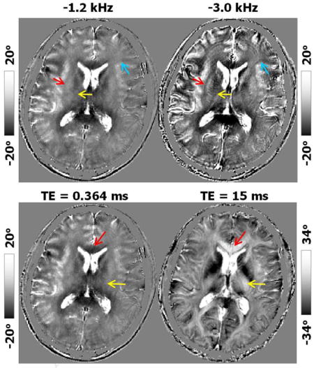
This reversed contrast between saturated signal at UTE and standard GRE at long TE can be further visualized by comparing the saturated signal acquired at gradually increasing echo times (Fig. 5). As the TE increased from 0.364 ms (Fig. 5a) to 15.0 ms (Fig. 5c) while using the same 3D radial trajectory, the phase of the saturated CSF components remained consistently large and positive, while overall gray matter gradually changed from positive to negative and white matter changed from negative to positive. Quantitatively, the mean frequency shift of the gray matter increased from −0.013 ppm at TE = 0.364 ms to 0.001 ppm at TE = 15 ms (Table 2 & Fig. 7). On the other hand, the mean frequency shift of the white matter decreased from 0.011 ppm to −0.001 ppm (Table 2). This trend is consistent in several specific white matter and gray matter anatomical regions (Table 2). Such a reversal of gray and white matter contrast can be clearly visualized in Fig. 5&7, as indicated e.g. in the GCC (red arrow in Fig. 5) and internal capsule (IC) (yellow arrow in Fig. 5). Similar TE-dependent phase contrast was also observed from the data acquired with a different spatial resolution (2×2×2 mm³) as shown in the Supplemental Fig. 1. The white gray matter contrast was completely reversed at TE = 15 ms compared to that at TE= 0.364 ms.

Figure 5.

Dependence of the saturated signal on TE (saturation frequency −1.2 kHz). A representative axial slice of normalized magnitude and phase images acquired at TE equals to (a) 0.364 ms, (b) 5 ms and (c) 15 ms. As TE increases, there is a gradual decrease in magnitude contrast. The intensity of CSF in the saturated magnitude images are non-zeros. On the other hand, phase contrast between gray and white matter reverses as the TE increases. At TE = 0.364 ms, white matter generally shows a negative phase shift (arrows); at TE = 15 ms, white matter shows a positive phase shift while CSF remains highly positive. Note that the magnitude and phase images at TE = 15 ms (c) are without saturation. Spatial resolution = 1×1×3 mm³.

Table 2.

Frequency shift of saturated signal as a function of TE and saturation frequency. For TE = 0.364 ms, the effective TE was assumed to be 1.14 ms to calculate the frequency shifts (θ = −2π f middot; TE_eff); for TE of 5.0 and 15.0 ms, the effect of finite readout duration was considered negligible. All frequency shifts were referenced to the mean phase of the whole brain (carrier frequency).

Frequency shift (ppm)		CSF	GM	WM	GCC	SCC	IC	EC	PU	CD
Sat Freq (kHz) (TE = 0.364 ms)	−1.2	−0.406	−0.013	0.011	0.046	0.057	0.038	0.002	−0.020	0.035
		(± 0.135)	(± 0.01)	(± 0.003)	(± 0.025)	(± 0.03)	(± 0.023)	(± 0.001)	(± 0.016)	(± 0.020)
	−1.8	−0.425	−0.013	0.025	0.059	0.072	0.052	0.015	−0.027	0.026
		(± 0.17)	(± 0.008)	(± 0.005)	(± 0.028)	(± 0.016)	(± 0.035)	(± 0.010)	(± 0.012)	(± 0.008)
	−2.4	−0.392	−0.019	0.028	0.067	0.088	0.050	0.016	−0.033	0.016
		(± 0.16)	(± 0.009)	(± 0.010)	(± 0.023)	(± 0.047)	(± 0.036)	(± 0.008)	(± 0.014)	(± 0.006)
	−3.0	−0.353	−0.020	0.031	0.073	0.102	0.052	0.016	−0.036	0.009
		(± 0.16)	(± 0.008)	(± 0.012)	(± 0.034)	(± 0.050)	(± 0.023)	(± 0.005)	(± 0.026)	(± 0.043)
TE (ms) (Sat Freq = −1.2 kHz)	0.364	−0.406	−0.013	0.011	0.046	0.057	0.038	0.002	−0.020	0.035
		(± 0.135)	(± 0.01)	(± 0.003)	(± 0.025)	(± 0.030)	(± 0.023)	(± 0.001)	(± 0.016)	(± 0.020)
	5.0	−0.372	−0.004	0.001	0.006	0.012	0.004	−0.004	−0.001	0.015
		(± 0.037)	(± 0.002)	(± 0.001)	(± 0.009)	(± 0.009)	(± 0.012)	(± 0.005)	(± 0.007)	(± 0.010)
	15.0	−0.328	0.001	−0.001	−0.013	−0.006	−0.004	−0.002	0.005	0.009
		(± 0.01)	(± 0.001)	(± 0.001)	(± 0.006)	(± 0.006)	(± 0.008)	(± 0.005)	(± 0.007)	(± 0.009)
TE (ms) (GRE w/o Sat)	15.0	−0.312	0.001	−0.003	−0.011	−0.010	−0.002	−0.002	0.009	0.010
		(± 0.006)	(± 0.006)	(± 0.006)	(± 0.005)	(± 0.007)	(± 0.012)	(± 0.007)	(± 0.007)	(±± 0.005)
Difference at TE=15ms	15.0	−0.016	0	0.002	−0.002	0.004	−0.002	0	−0.004	−0.001

Note: CSF – cerebral spinal fluid; GM – gray matter; WM – white matter; GCC – genu corpus callosum; SCC – splenium corpus callosum; IC – internal capsule; EC – external capsule; PU – putamen; CD – caudate nucleus.

Figure 7.

Frequency shift of saturated signal as a function of saturation frequency (a) and TE (b). (a) At TE = 0.364 ms, increasing saturation frequency (in amplitude) resulted in a more positive shift in white mater and a more negative shift in gray matter, thus improving gray-white matter contrast. (b) On the other hand, increasing TE resulted in reduced contrast in the saturated signal. The contrast also reversed at TE = 15 ms compared to TE = 0.364 ms. GM – gray matter; WM – white matter; GCC – genu corpus callosum; SCC – splenium corpus callosum; IC – internal capsule; EC – external capsule; PU – putamen; CD – caudate nucleus.

The effect of MT and direct saturation are evaluated at longer TE when the short and ultra-short-T2 species have decayed away. As shown in the Supplemental Fig. 2, at TE = 15 ms, gradient echo phase images demonstrated similar contrast with or without saturation which was different from those at UTE (Fig. 4b). A subtraction of the phase images with or without saturation showed small difference except at the tissue boundary. Overall, the phase difference was −0.08° for white matter, 0.08° for gray matter and 0.14° for CSF. These differences were nearly two-orders of magnitude smaller than those at UTE. This suggests that the UTE phase contrast is dominated by the short and ultra-short-T2 species.

Dependence on saturation frequency

When the saturation frequency was increased (in absolute value) from −1.2 kHz to −3.0 kHz, the signal intensity in the MT ratio reduced gradually (Fig. 6a). However, phase contrast clearly increased as the saturation frequency increased (Fig. 6b). While the underlying mean frequency shift of all white matter regions increased from 0.011 ppm to 0.031 ppm, the mean frequency shift of gray matter decreased from −0.013 ppm to −0.020 ppm, thus improving gray-white matter contrast (Fig. 7a) CSF frequency shift also increased from −0.406 ppm to −0.353 ppm and demonstrated consistently to be the largest shift in absolute value. As the saturation frequency increases, white matter fiber bundles became more easily identifiable in the phase images as indicated, e.g., by the red arrow for the external capsule (EC) and the yellow arrow for IC (Fig. 6b). The boundaries between gray and white matter also became sharper (blue arrow in Fig. 6b). When the sign of the saturation frequency was flipped, the basic characteristics of the phase in the saturated components did not change (Supplemental Fig. 3). Specifically, CSF exhibited the highest phase shift followed by gray matter; white matter generally exhibited negative phase shift (Supplemental Fig. 3). A subtraction of the phase between negative and positive saturation frequency seemed to indicate that negative saturation frequency resulted in slightly more negative phase in the saturated signals. However, when evaluated quantitatively, the mean difference was only −0.03° in the white matter and 0.7° in the gray matter (Supplemental Fig. 3c).

Figure 6.

Image contrast of the saturated signal as a function of saturation frequency (TE = 0.364 ms, spatial resolution = 1×1×3 mm³). (a) MT ratio images with four different saturation frequencies. Contrasts are similar across the frequencies although the SNR decreases as the saturation frequency increases. (b) The corresponding phase images show increasing tissue contrast as the saturation frequency increases, for example, in the external capsule (red arrow), internal capsule (yellow arrow) and the boundaries between gray and white matter in the frontal cortex (blue arrow). White matter shows increasingly more negative phase shift as the saturation frequency increases.

As shown in Fig. 8, the MT ratio calculated from magnitude signal decreases significantly as the saturation frequency increases from −1.0 kHz to −15 kHz. However, phase contrast shows a different trend compared to the MT ratio images. The anatomical details with saturation pulse at −15 kHz are difficult to visualize.

Figure 8.

Image contrast of the saturated signal as a function of saturation frequency (TE = 0.2 ms). (a) MT ratio images with five different saturation frequencies. SNR of the MT ratio images decreases as the saturation frequency increases. (b) Phase contrast shows a different trend compared to the MT ratio images. At −15 kHz, Both MT effect and phase contrast are invisible Spatial resolution = 1×1×3 mm³.

UTE phase contrast in MS

The magnitude, MT ratio and phase images of saturated components using UTE sequence in an MS patient are shown in Fig. 9a–c. The MS lesion was identified based on its hypointensity in the T1 and hyperintensity in the FLAIR images as shown in Fig. 9e&f. Similar reversed contrast between the saturated signal at UTE and longer TE was observed. We expect that when demyelination occurs in the MS lesions, the frequency shift of the saturated signals in these lesions will become more negative, appearing similar to that of CSF. In this case there was such a shift, resulting in a more positive phase shift as shown by the red arrows in Fig. 9c. The UTE phase image provides excellent visualization of the MS lesion, which allows for the differentiation of lesions from the surrounding normal white matter tissues, while the contrast is greatly reduced in magnitude and MT ratio images at a longer TE of 7.66 ms. Similar strong phase contrast at UTE in another MS patient was observed as shown in the Supplemental Fig. 5.

Figure 9.

Dependence of the saturated signal on TE in an MS patient. (a) Magnitude images at different TEs. (b) MT ratio maps at different TEs. (c) Phase images at different TEs. (d) R2* map. (e) T1 image. (f) FLAIR image. At TE = 0.226 ms, MS lesion shows a strong contrast with surroundings. As TE increases, phase contrast between the lesion and surrounding white matter decreases gradually as pointed out by the red arrow in c. The phase contrast between gray and white matter also decreases as TE increases (blue arrows in c). The MS lesion was identified based on its hypointensity in the T1 and hyperintensity in the FLAIR images (e&f).

Discussion

We showed that, with off-resonance saturation pulses, brain tissues exhibited visible phase contrast even at a TE as short as 106 μs at 7 T. The phase properties of the saturated signals were evaluated by subtracting signals with saturation from signals without saturation. We expect the off-resonance pulses to create direct saturation of ultra-short-T2 components and indirect saturation of longer-T2 components via MT. This evaluation led to several unique findings: 1) phase contrast of saturated components between gray and white matter is reversed compared to that of long-T2 signals; 2) off-resonance saturation has minimal effects on phase at long echo times; 3) phase contrast of the saturated signal increases as the saturation frequency increases (up to −3 kHz in this study); 4) phase contrast is completely invisible at −15 kHz; 5) phase contrast at UTE in MS patients allowed better differentiation of lesions from the surrounding normal white matter tissues than that at long TE (e.g. 7.66 ms). Compared with MT ratio images, we speculate that the majority of the phase contrast in the saturated signals was a combination result of magnetic susceptibility and indirect MT saturation via the short and ultra-short-T2 components, as described below.

Sources of phase contrast at UTE

Gradient-echo phase images are commonly acquired at long echo times as phase reaches optimal SNR at TE = T2*. A typical TE used for phase imaging is in the range of 10–15 ms at 7 T and about 40 ms at 3 T. However, at such long TE, phase contrast is mainly dominated by long-T2 species that consist of mainly mobile water protons. A major benefit of UTE imaging is the ability to acquire tissue signals of extremely short T2 relaxation times. In the white matter, these ultra-short-T2 signals may originate from water confined in myelin sheaths, bounded water and immobile protons in lipids and proteins (Horch et al., 2011; Wilhelm et al., 2012b). UTE will also capture short-T2 signals originating from bounded water that have decayed at conventional phase imaging TEs.

The phase of a voxel measured in MRI is the phase of the complex signal from that voxel ∠ Σ_nμ_nexp(−i2πf_nTE +ϕ_n), where ∠ denotes the phase of a complex number, Σ_n is summation over all spin isochromats in the voxel, μ_n denotes the strength of the magnetization, TE denotes echo time, f_n is the Larmor frequency experienced by a particular spin isochromat. When off-resonance pulses were applied to selectively saturate macromolecular protons, a portion of the complex signal was removed from the total signal in the voxel. As a result, the saturated spins will introduce a phase shift in the sampled signal. In addition, bounded water may undergo both dipole-dipole cross relaxation as well as chemical exchange with macromolecular ¹H nuclei. Bounded water also interfaces with free water on its outer surface. This chemical exchange between protons and water has been reported to cause a phase shift of the signal (Luo et al., 2010).

To obtain the phase images of the saturated components, subtraction is performed between the images acquired with and without saturation. Two methods of performing this subtraction can be used: direct phase subtraction and complex subtraction. The direct phase-difference method subtracts the phase signal obtained from two acquisitions. The complex-difference method is performed by calculating the phase of the complex difference signal. Based on the multi-component signal model shown in the previous paragraph, the complex-difference method is the correct method for computing the phase of the saturated component. More details can be found in the Supplemental Fig. 6.

There are several factors that may affect the observed phase contrast: MT or chemical exchange, and magnetic susceptibility. Susceptibility of biomolecules is on the order of −0.1 ppm (Li et al., 2012). For example, membrane lipids have susceptibility at around −0.223 ppm (Lounila et al., 1994) which is on the order of the observed frequency shift in the saturated signals but is of opposite sign (Table 2). Although the anisotropy of the diamagnetic susceptibility of myelin lipids may introduce a positive frequency shift inside the axons, axonal water is generally considered to have long T2 relaxation times. Proton exchange between protein and water has been reported to cause a positive frequency shift in the white matter (Shmueli et al., 2011). However, this shift is on the order of 0.01 ppm and cannot fully account for the observed shift (~0.4 ppm when referenced to CSF).

The off-resonance saturation RF pulses will directly saturate ultra-short-T2 components and indirectly saturate nearby components via MT. At a saturation of frequency of −1.2 kHz with the saturation pulse bandwidth of 1.0 kHz, we expect that components of the broad peak with linewidths greater than 1.4 kHz (i.e. 2×(1.2 – 0.5) kHz), which corresponds to T2 ≈ 230 μs, will experience substantial direct saturation, while only components with very broad linewidths greater than 5 kHz (T2 ≤ 65 μs) will experience substantial direct saturation using −3.0 kHz saturation frequency. Components with ultra-short T2 ≤ 100 μs are difficult to visualize, even with UTE, given our shortest TE of 106 μs and a readout window of 1.024 ms. However, our data showed that UTE phase contrast increased up to the −3.0 kHz saturation frequency, suggesting that indirect saturation by MT may also contribute significantly to phase contrast of the saturated signals. Further, at even larger off-resonance frequencies (i.e., −10 kHz), the direct saturation should contribute little to the phase contrast but we still observed clear phase contrast between gray and white matter that suggests indirect saturation is the primary mechanism creating phase contrast (Fig. 8). The experiments with two frequencies of opposite signs (−1.2 kHz and 1.2 kHz) showed that the general characteristics of the phase contrast in the saturated signal remain the same instead of with opposite signs (Supplemental Fig. 3), further supporting that indirect saturation via MT is the strongest contributor to the phase contrast. The experiments with varying saturation pulse bandwidths showed that the phase contrast increased with a narrower saturation pulse bandwidth (Supplemental Fig. 4), also suggesting that indirect saturation via MT is the strongest contributor to the phase contrast.

In the white matter, these immobile protons are expected to reside in the myelin. Myelin is rich in lipids (~70% dry weight) and proteins (~30% dry weight) (Baumann and Pham-Dinh, 2001). On average, lipids may occupy 10–20% of the volume in the white matter (Baumann and Pham-Dinh, 2001; Woodard and White, 1986). A recent study by Horch et al (Horch et al., 2011) showed that T2s in myelinated white matter can be as short as 10 μs, with several ultra-short T2 < 1 ms components. They further suggested that this ultra-short T2 signal originates from methylene 1H in myelin membranes (Horch et al., 2011). Protons exist in different chemical bounds such as the amide (NH) group, methylene (CH2) group, hydroxyl (OH) group and carboxyl (CO2H) group. Each group exhibits a different range of chemical shifts. For example, the amide protons have a chemical shift around 8 ppm (Zhou et al., 2003a; Zhou et al., 2003b) while the other groups have smaller shifts in the range of 1–5 ppm. In comparison, water at 37°C has a shift of 4.7 ppm referenced to Tetramethylsilane. Although we cannot identify the specific group or groups of protons that are responsible due to the lack of absolute frequency reference, the observed positive frequency shift in the white matter can be potentially attributed to the various protons in those lipids and proteins.

As shown in Supplemental Fig. 7, with saturation, the magnitude signal intensity of the white matter decreased significantly relative to gray matter. The MT ratio in (b) was calculated as (Mag(off) – Mag(on))/Mag(off). Surprisingly, the intensity of CSF on the MT ratio images is non-zero although it is relatively small compared to white matter. Choroid plexus exhibits brighter MT ratio while the fluid shows a relatively lower intensity as shown in Supplemental Fig. 7b. By segmenting the CSF regions, Supplemental Fig. 7c clearly shows the saturated CSF in the MT ratio image by the off-resonance pulses. Clear anatomical contrast was observed within the ventricle as pointed by arrows. Supplemental Fig. 7d shows phase images without and with saturation and the direct phase difference between the two were shown in Supplemental Fig. 7e. The direct phase difference is relatively small. Combining with MT ratio as shown in Supplemental Fig. 7c, we concluded that the complex signals without and with saturation pulses have the similar phase angle and only with minor magnitude differences. Thus, the phase of the complex subtraction is equal to the initial phase without saturation. Supplemental Fig. 7f shows the phase image computed by the complex difference method and fluid is similar to the initial phase as shown in Supplemental Fig. 7d. In addition, the anatomical contrast of ventricle revealed on phase image in (f) is highly consistent with that on the magnitude image (Supplemental Fig. 7c). Note that CSF is not purely with fluid since CSF also contains ~0.3% of plasma proteins (BOCK, 1973), which could contribute to the non-zero values of the MT ratio within the ventricle.

Pool selective phase contrast

One implication of our findings is the possibility to generate more pool-specific phase contrast. By comparing phase contrast measured with and without saturation and at different echo times, it is possible to examine phase signals of each pool signals that have shown to exhibit different T2 relaxation rates. This pool specific phase contrast may especially be useful for detecting demyelination diseases such as multiple sclerosis. While previous studies based on phase and susceptibility maps measured at long TE have shown that the diamagnetic susceptibility and susceptibility anisotropy of white matter originates from myelin lipids, the availability of UTE phase may further improve the sensitivity and specificity. Sensitivity may be improved due to the significantly increased frequency shift while specificity can be improved because the signal originates directly from the short and ultra-short T2 protons in the myelin.

While the magnitude image of the saturated signals also provides high gray and white matter contrast in general, the magnitude contrast is similar to T1 weighted images. White matter generally appears homogeneously hyperintense. Phase contrast, on the other hand, provides very different and additional unique information. For example, there were significant heterogeneities in the phase of white matter. The GCC and SCC tend to show much larger phase shifts than other white matter regions. The boundaries between gray and white matter also exhibit much higher frequency shifts, especially in the cortex (pointed by blue arrows in Fig. 7&9). In addition, phase contrast also exhibits stronger dependence on saturation frequency while magnitude only shows reduced SNR, but maintains generally the same contrast.

There are multiple ways to achieve such a pool-selective phase contrast. While we have used the application of off-resonance pulses for selective saturation of the broad ultra-short-T2 spectrum, saturation may also be realized by long-T2 suppression methods. Long-T2 suppression can be achieved by subtracting two echoes with slightly different echo times or by using specially designed long-T2 suppression RF pulses (Larson et al., 2006). Long-T2 signal may also be suppressed with a conventional inversion pulse applied before imaging (Du et al., 2014; Oh et al., 2013). Contrast agents are another way to suppress certain signal pools. For example, Gadolinium based T1-shortening agents have been used to enhance phase contrast between gray and white matter in perfusion-fixed mouse brains (Dibb et al., 2014).

Limitations

Phase in UTE images is more complex than conventional gradient-echo images due to additional phase accumulation during the radial readout. A theoretical framework was recently published, with meniscus imaging results (Carl and Chiang, 2012), but it requires an estimate of the object size for a given frequency shift. The point spread function analysis presented here assumes a point object, i.e. that the object size is smaller than or equal to the resolution size. The slight difference we found between these two models and the assumptions required for their generation indicate that the UTE phase versus frequency relationship is still an open question. Further correction of the TE will not fundamentally change our conclusions.

In the present study, the observed phase contrast at UTE is a combination of direct saturation and indirect MT effect and we speculate that the major contribution comes from indirect MT saturation. Further investigation of the origins of the phase contrast generated by the direct saturation and indirect MT is required in this area. For example, Deuterium water (D2O) was used to exchange tissue water and hence directly quantify the MR signal of myelin at UTE (Wilhelm et al., 2012a). D2O exchange studies of brain white matter samples need be conducted to explore the potential for direct quantification of phase contrast from myelin water by UTE under the assumption that the exchange between bounded water and free water contributes minimally to MT when D2O completely exchanges the free water in the white matter. Specifically, comparing the phase difference images of the saturated components without and with the specimen immersed in D2O may further our understanding on the relative contributions of direct saturation and indirect MT. Their contributions to the phase contrast at different echo times will also be investigated.

In this study, one limitation was the limited number of MS patients who underwent the clinical scans at 3 T. Our preliminary data demonstrate that the UTE phase image allows for better differentiation of MS lesions from the surrounding normal white matter compared to the phase images at longer TEs. The strong phase contrast at UTE suggests that the demyelination may occur at ultrashort T2 components within white matter. It indicates that UTE phase imaging may provide valuable new information to help characterize MS lesions. However, caution must be taken when interpreting lesion detections based on phase/frequency imaging since heterogeneity exists in the MS lesions (Li et al., 2016). As reported in the previous studies, using conventional phase imaging at a longer TE of 12 ms at 7 T, the isointense MS lesions with no edge/rim accounting for 42.2% of total lesions are invisible on the frequency images (Li et al., 2016). Little is known about the ability of UTE phase imaging for the detection of these invisible lesions. However, this can be considered in future work conducting UTE phase imaging in a larger cohort of patients with MS.

Conclusion

Until now, phase contrast of the brain has been largely generated at long TE. UTE imaging offers advantages in being able to directly image tissues with T2 values less than a few milliseconds. In the brain, ultra-short-T2 components are present in white matter – believed to be associated with myelin – as well as in connective tissues and calcifications, and these are known to be altered in neurodegenerative diseases and other neurological pathologies. We have shown that off-resonance saturation together with UTE offers a new way to generate phase contrast in the brain and may provide valuable new information helpful for probing tissue microstructure.

References

- Andrews T, Lancaster JL, Dodd SJ, Contreras-Sesvold C, Fox PT. Testing the three-pool white matter model adapted for use with T2 relaxometry. Magn Reson Med. 2005;54:449–454. doi: 10.1002/mrm.20599. [DOI] [PubMed] [Google Scholar]
- Andrews TJ, Osborne MT, Does MD. Diffusion of myelin water. Magn Reson Med. 2006;56:381–385. doi: 10.1002/mrm.20945. [DOI] [PubMed] [Google Scholar]
- Assaf Y, Freidlin RZ, Rohde GK, Basser PJ. New modeling and experimental framework to characterize hindered and restricted water diffusion in brain white matter. Magn Reson Med. 2004;52:965–978. doi: 10.1002/mrm.20274. [DOI] [PubMed] [Google Scholar]
- Avram AV, Guidon A, Song AW. Myelin water weighted diffusion tensor imaging. NeuroImage. 2010;53:132–138. doi: 10.1016/j.neuroimage.2010.06.019. [DOI] [PubMed] [Google Scholar]
- Baumann N, Pham-Dinh D. Biology of oligodendrocyte and myelin in the mammalian central nervous system. Physiol Rev. 2001;81:871–927. doi: 10.1152/physrev.2001.81.2.871. [DOI] [PubMed] [Google Scholar]
- Beatty PJ, Nishimura DG, Pauly JM. Rapid gridding reconstruction with a minimal oversampling ratio. IEEE Trans Med Imaging. 2005;24:799–808. doi: 10.1109/TMI.2005.848376. [DOI] [PubMed] [Google Scholar]
- Boucneau T, Cao P, Tang S, Han M, Xu D, Henry RG, Larson PE. In vivo characterization of brain ultrashort-T2 components. Magnetic resonance in medicine. 2017 doi: 10.1002/mrm.27037. [DOI] [PMC free article] [PubMed] [Google Scholar]
- Carl M, Chiang JT. Investigations of the origin of phase differences seen with ultrashort TE imaging of short T2 meniscal tissue. Magn Reson Med. 2012;67:991–1003. doi: 10.1002/mrm.23075. [DOI] [PubMed] [Google Scholar]
- Chen WC, Foxley S, Miller KL. Detecting microstructural properties of white matter based on compartmentalization of magnetic susceptibility. NeuroImage. 2013;70:1–9. doi: 10.1016/j.neuroimage.2012.12.032. [DOI] [PMC free article] [PubMed] [Google Scholar]
- Cronin MJ, Wang N, Decker KS, Wei H, Zhu WZ, Liu C. Exploring the origins of echo-time-dependent quantitative susceptibility mapping (QSM) measurements in healthy tissue and cerebral microbleeds. NeuroImage. 2017;149:98–113. doi: 10.1016/j.neuroimage.2017.01.053. [DOI] [PMC free article] [PubMed] [Google Scholar]
- Deoni SC, Dean DC, 3rd, O’Muircheartaigh J, Dirks H, Jerskey BA. Investigating white matter development in infancy and early childhood using myelin water faction and relaxation time mapping. NeuroImage. 2012;63:1038–1053. doi: 10.1016/j.neuroimage.2012.07.037. [DOI] [PMC free article] [PubMed] [Google Scholar]
- Deoni SC, Matthews L, Kolind SH. One component? Two components? Three? The effect of including a nonexchanging “free” water component in multicomponent driven equilibrium single pulse observation of T1 and T2. Magn Reson Med. 2013;70:147–154. doi: 10.1002/mrm.24429. [DOI] [PMC free article] [PubMed] [Google Scholar]
- Deoni SC, Rutt BK, Arun T, Pierpaoli C, Jones DK. Gleaning multicomponent T1 and T2 information from steady-state imaging data. Magn Reson Med. 2008a;60:1372–1387. doi: 10.1002/mrm.21704. [DOI] [PubMed] [Google Scholar]
- Deoni SC, Rutt BK, Jones DK. Investigating exchange and multicomponent relaxation in fully-balanced steady-state free precession imaging. J Magn Reson Imaging. 2008b;27:1421–1429. doi: 10.1002/jmri.21079. [DOI] [PubMed] [Google Scholar]
- Dibb R, Li W, Cofer W, Liu C. Microstructural origins of gadolinium-enhanced susceptibility contrast and anisotropy. Magn Reson Med Early View. 2014 doi: 10.1002/mrm.25082. [DOI] [PMC free article] [PubMed] [Google Scholar]
- Does MD, Beaulieu C, Allen PS, Snyder RE. Multi-component T1 relaxation and magnetisation transfer in peripheral nerve. Magn Reson Imaging. 1998;16:1033–1041. doi: 10.1016/s0730-725x(98)00139-8. [DOI] [PubMed] [Google Scholar]
- Does MD, Gore JC. Compartmental study of diffusion and relaxation measured in vivo in normal and ischemic rat brain and trigeminal nerve. Magn Reson Med. 2000;43:837–844. doi: 10.1002/1522-2594(200006)43:6<837::aid-mrm9>3.0.co;2-o. [DOI] [PubMed] [Google Scholar]
- Does MD, Gore JC. Compartmental study of T(1) and T(2) in rat brain and trigeminal nerve in vivo. Magn Reson Med. 2002;47:274–283. doi: 10.1002/mrm.10060. [DOI] [PubMed] [Google Scholar]
- Dortch RD, Harkins KD, Juttukonda MR, Gore JC, Does MD. Characterizing inter-compartmental water exchange in myelinated tissue using relaxation exchange spectroscopy. Magn Reson Med. 2012 doi: 10.1002/mrm.24571. [DOI] [PMC free article] [PubMed] [Google Scholar]
- Du J, Ma G, Li S, Carl M, Szeverenyi NM, Vandenberg S, Corey-Bloom J, Bydder GM. Ultrashort echo time (UTE) magnetic resonance imaging of the short T2 components in white matter of the brain using a clinical 3T scanner. NeuroImage. 2014;87:32–41. doi: 10.1016/j.neuroimage.2013.10.053. [DOI] [PMC free article] [PubMed] [Google Scholar]
- Du J, Takahashi AM, Bydder M, Chung CB, Bydder GM. Ultrashort TE imaging with off-resonance saturation contrast (UTE-OSC) Magn Reson Med. 2009;62:527–531. doi: 10.1002/mrm.22007. [DOI] [PubMed] [Google Scholar]
- Du YP, Chu R, Hwang D, Brown MS, Kleinschmidt-DeMasters BK, Singel D, Simon JH. Fast multislice mapping of the myelin water fraction using multicompartment analysis of T2* decay at 3T: a preliminary postmortem study. Magn Reson Med. 2007;58:865–870. doi: 10.1002/mrm.21409. [DOI] [PubMed] [Google Scholar]
- Dula AN, Gochberg DF, Valentine HL, Valentine WM, Does MD. Multiexponential T2, magnetization transfer, and quantitative histology in white matter tracts of rat spinal cord. Magn Reson Med. 2010;63:902–909. doi: 10.1002/mrm.22267. [DOI] [PMC free article] [PubMed] [Google Scholar]
- Duyn JH, van Gelderen P, Li TQ, de Zwart JA, Koretsky AP, Fukunaga M. High-field MRI of brain cortical substructure based on signal phase. Proc Natl Acad Sci U S A. 2007;104:11796–11801. doi: 10.1073/pnas.0610821104. [DOI] [PMC free article] [PubMed] [Google Scholar]
- Gatehouse PD, Bydder GM. Magnetic resonance imaging of short T2 components in tissue. Clin Radiol. 2003;58:1–19. doi: 10.1053/crad.2003.1157. [DOI] [PubMed] [Google Scholar]
- Glover GH, Pauly JM. Projection reconstruction techniques for reduction of motion effects in MRI. Magn Reson Med. 1992;28:275–289. doi: 10.1002/mrm.1910280209. [DOI] [PubMed] [Google Scholar]
- Gold GE, Thedens DR, Pauly JM, Fechner KP, Bergman G, Beaulieu CF, Macovski A. MR imaging of articular cartilage of the knee: new methods using ultrashort TEs. AJR Am J Roentgenol. 1998;170:1223–1226. doi: 10.2214/ajr.170.5.9574589. [DOI] [PubMed] [Google Scholar]
- Henkelman RM, Stanisz GJ, Graham SJ. Magnetization transfer in MRI: a review. NMR Biomed. 2001;14:57–64. doi: 10.1002/nbm.683. [DOI] [PubMed] [Google Scholar]
- Horch RA, Gore JC, Does MD. Origins of the ultrashort-T2 1H NMR signals in myelinated nerve: a direct measure of myelin content? Magn Reson Med. 2011;66:24–31. doi: 10.1002/mrm.22980. [DOI] [PMC free article] [PubMed] [Google Scholar]
- Hwang D, Kim DH, Du YP. In vivo multi-slice mapping of myelin water content using T2* decay. NeuroImage. 2010;52:198–204. doi: 10.1016/j.neuroimage.2010.04.023. [DOI] [PubMed] [Google Scholar]
- Kucharczyk W, Macdonald PM, Stanisz GJ, Henkelman RM. Relaxivity and magnetization transfer of white matter lipids at MR imaging: importance of cerebrosides and pH. Radiology. 1994;192:521–529. doi: 10.1148/radiology.192.2.8029426. [DOI] [PubMed] [Google Scholar]
- Lancaster JL, Andrews T, Hardies LJ, Dodd S, Fox PT. Three-pool model of white matter. J Magn Reson Imaging. 2003;17:1–10. doi: 10.1002/jmri.10230. [DOI] [PubMed] [Google Scholar]
- Larson PE, Gurney PT, Nayak K, Gold GE, Pauly JM, Nishimura DG. Designing long-T2 suppression pulses for ultrashort echo time imaging. Magn Reson Med. 2006;56:94–103. doi: 10.1002/mrm.20926. [DOI] [PMC free article] [PubMed] [Google Scholar]
- Larson PE, Han M, Krug R, Jakary A, Nelson SJ, Vigneron DB, Henry RG, McKinnon G, Kelley DA. Ultrashort echo time and zero echo time MRI at 7T. Magnetic Resonance Materials in Physics, Biology and Medicine. 2016;29:359–370. doi: 10.1007/s10334-015-0509-0. [DOI] [PMC free article] [PubMed] [Google Scholar]
- Larson PZ, Gurney PT, Nishimura DG. Anisotropic field-of-views in radial imaging. IEEE Trans Med Imaging. 2008;27:47–57. doi: 10.1109/TMI.2007.902799. [DOI] [PubMed] [Google Scholar]
- Lee J, Shmueli K, Kang BT, Yao B, Fukunaga M, van Gelderen P, Palumbo S, Bosetti F, Silva AC, Duyn JH. The contribution of myelin to magnetic susceptibility-weighted contrasts in high-field MRI of the brain. NeuroImage. 2012;59:3967–3975. doi: 10.1016/j.neuroimage.2011.10.076. [DOI] [PMC free article] [PubMed] [Google Scholar]
- Li W, Avram AV, Wu B, Xiao X, Liu C. Integrated Laplacian-based phase unwrapping and background phase removal for quantitative susceptibility mapping. NMR in Biomedicine. 2013 doi: 10.1002/nbm.3056. n/a-n/a. [DOI] [PMC free article] [PubMed] [Google Scholar]
- Li W, Wu B, Avram AV, Liu C. Magnetic susceptibility anisotropy of human brain in vivo and its molecular underpinnings. NeuroImage. 2012;59:2088–2097. doi: 10.1016/j.neuroimage.2011.10.038. [DOI] [PMC free article] [PubMed] [Google Scholar]
- Li W, Wu B, Liu C. Quantitative susceptibility mapping of human brain reflects spatial variation in tissue composition. NeuroImage. 2011;55:1645–1656. doi: 10.1016/j.neuroimage.2010.11.088. [DOI] [PMC free article] [PubMed] [Google Scholar]
- Li X, Harrison DM, Liu H, Jones CK, Oh J, Calabresi PA, van Zijl P. Magnetic susceptibility contrast variations in multiple sclerosis lesions. Journal of magnetic resonance imaging. 2016;43:463–473. doi: 10.1002/jmri.24976. [DOI] [PMC free article] [PubMed] [Google Scholar]
- Liu C. Susceptibility tensor imaging. Magn Reson Med. 2010;63:1471–1477. doi: 10.1002/mrm.22482. [DOI] [PMC free article] [PubMed] [Google Scholar]
- Liu C, Li W. Imaging neural architecture of the brain based on its multipole magnetic response. NeuroImage. 2013;67:193–202. doi: 10.1016/j.neuroimage.2012.10.050. [DOI] [PMC free article] [PubMed] [Google Scholar]
- Liu C, Li W, Johnson GA, Wu B. High-field (9.4 T) MRI of brain dysmyelination by quantitative mapping of magnetic susceptibility. NeuroImage. 2011;56:930–938. doi: 10.1016/j.neuroimage.2011.02.024. [DOI] [PMC free article] [PubMed] [Google Scholar]
- Liu C, Li W, Tong KA, Yeom KW, Kuzminski S. Susceptibility-weighted imaging and quantitative susceptibility mapping in the brain. Journal of magnetic resonance imaging. 2015a;42:23–41. doi: 10.1002/jmri.24768. [DOI] [PMC free article] [PubMed] [Google Scholar]
- Liu C, Wei H, Gong NJ, Cronin M, Dibb R, Decker K. Quantitative susceptibility mapping: contrast mechanisms and clinical applications. Tomography: a journal for imaging research. 2015b;1:3. doi: 10.18383/j.tom.2015.00136. [DOI] [PMC free article] [PubMed] [Google Scholar]
- Lounila J, Ala-Korpela M, Jokisaari J, Savolainen MJ, Kesaniemi YA. Effects of orientational order and particle size on the NMR line positions of lipoproteins. Phys Rev Lett. 1994;72:4049–4052. doi: 10.1103/PhysRevLett.72.4049. [DOI] [PubMed] [Google Scholar]
- Luo J, He X, Andre’d’Avignon D, Ackerman JJ, Yablonskiy DA. Protein-induced water 1 H MR frequency shifts: contributions from magnetic susceptibility and exchange effects. Journal of Magnetic Resonance. 2010;202:102–108. doi: 10.1016/j.jmr.2009.10.005. [DOI] [PMC free article] [PubMed] [Google Scholar]
- Oh SH, Bilello M, Schindler M, Markowitz CE, Detre JA, Lee J. Direct visualization of short transverse relaxation time component (ViSTa) NeuroImage. 2013;83C:485–492. doi: 10.1016/j.neuroimage.2013.06.047. [DOI] [PMC free article] [PubMed] [Google Scholar]
- Peled S, Cory DG, Raymond SA, Kirschner DA, Jolesz FA. Water diffusion, T(2), and compartmentation in frog sciatic nerve. Magn Reson Med. 1999;42:911–918. doi: 10.1002/(sici)1522-2594(199911)42:5<911::aid-mrm11>3.0.co;2-j. [DOI] [PMC free article] [PubMed] [Google Scholar]
- Rauscher A, Sedlacik J, Barth M, Mentzel HJ, Reichenbach JR. Magnetic susceptibility-weighted MR phase imaging of the human brain. AJNR Am J Neuroradiol. 2005;26:736–742. [PMC free article] [PubMed] [Google Scholar]
- Robinson SD, Bredies K, Khabipova D, Dymerska B, Marques JP, Schweser F. An illustrated comparison of processing methods for MR phase imaging and QSM: combining array coil signals and phase unwrapping. NMR in Biomedicine. 2017:30. doi: 10.1002/nbm.3601. [DOI] [PMC free article] [PubMed] [Google Scholar]
- Robson MD, Gatehouse PD, Bydder M, Bydder GM. Magnetic resonance: an introduction to ultrashort TE (UTE) imaging. J Comput Assist Tomogr. 2003;27:825–846. doi: 10.1097/00004728-200311000-00001. [DOI] [PubMed] [Google Scholar]
- Sati P, van Gelderen P, Silva AC, Reich DS, Merkle H, de Zwart JA, Duyn JH. Micro-compartment specific T2* relaxation in the brain. NeuroImage. 2013;77:268–278. doi: 10.1016/j.neuroimage.2013.03.005. [DOI] [PMC free article] [PubMed] [Google Scholar]
- Schweser F, Deistung A, Lehr BW, Reichenbach JR. Quantitative imaging of intrinsic magnetic tissue properties using MRI signal phase: an approach to in vivo brain iron metabolism? NeuroImage. 2011;54:2789–2807. doi: 10.1016/j.neuroimage.2010.10.070. [DOI] [PubMed] [Google Scholar]
- Shmueli K, Dodd S, Gelderen P, Duyn J. Investigating lipids as a source of chemical exchange-induced MRI frequency shifts. NMR in Biomedicine. 2016 doi: 10.1002/nbm.3525. [DOI] [PMC free article] [PubMed] [Google Scholar]
- Shmueli K, Dodd SJ, Li TQ, Duyn JH. The contribution of chemical exchange to MRI frequency shifts in brain tissue. Magn Reson Med. 2011;65:35–43. doi: 10.1002/mrm.22604. [DOI] [PMC free article] [PubMed] [Google Scholar]
- Smith SM, Jenkinson M, Woolrich MW, Beckmann CF, Behrens TE, Johansen-Berg H, Bannister PR, De Luca M, Drobnjak I, Flitney DE, Niazy RK, Saunders J, Vickers J, Zhang Y, De Stefano N, Brady JM, Matthews PM. Advances in functional and structural MR image analysis and implementation as FSL. NeuroImage. 2004;23(Suppl 1):S208–219. doi: 10.1016/j.neuroimage.2004.07.051. [DOI] [PubMed] [Google Scholar]
- Stanisz GJ, Kecojevic A, Bronskill MJ, Henkelman RM. Characterizing white matter with magnetization transfer and T(2) Magn Reson Med. 1999;42:1128–1136. doi: 10.1002/(sici)1522-2594(199912)42:6<1128::aid-mrm18>3.0.co;2-9. [DOI] [PubMed] [Google Scholar]
- Sukstanskii AL, Yablonskiy DA. On the role of neuronal magnetic susceptibility and structure symmetry on gradient echo MR signal formation. Magn Reson Med. 2013 doi: 10.1002/mrm.24629. [DOI] [PMC free article] [PubMed] [Google Scholar]
- Tyler DJ, Robson MD, Henkelman RM, Young IR, Bydder GM. Magnetic resonance imaging with ultrashort TE (UTE) PULSE sequences: technical considerations. J Magn Reson Imaging. 2007;25:279–289. doi: 10.1002/jmri.20851. [DOI] [PubMed] [Google Scholar]
- van Gelderen P, de Zwart JA, Lee J, Sati P, Reich DS, Duyn JH. Nonexponential T(2) decay in white matter. Magn Reson Med. 2012;67:110–117. doi: 10.1002/mrm.22990. [DOI] [PMC free article] [PubMed] [Google Scholar]
- Wei H, Dibb R, Zhou Y, Sun Y, Xu J, Wang N, Liu C. Streaking artifact reduction for quantitative susceptibility mapping of sources with large dynamic range. NMR in Biomedicine. 2015;28:1294–1303. doi: 10.1002/nbm.3383. [DOI] [PMC free article] [PubMed] [Google Scholar]
- Wei H, Xie L, Dibb R, Li W, Decker K, Zhang Y, Johnson GA, Liu C. Imaging whole-brain cytoarchitecture of mouse with MRI-based quantitative susceptibility mapping. NeuroImage. 2016;137:107–115. doi: 10.1016/j.neuroimage.2016.05.033. [DOI] [PMC free article] [PubMed] [Google Scholar]
- Wei H, Zhang Y, Gibbs E, Chen NK, Wang N, Liu C. Joint 2D and 3D phase processing for quantitative susceptibility mapping: application to 2D echo-planar imaging. NMR in Biomedicine. 2017:30. doi: 10.1002/nbm.3501. [DOI] [PubMed] [Google Scholar]
- Wharton S, Bowtell R. Fiber orientation-dependent white matter contrast in gradient echo MRI. Proc Natl Acad Sci U S A. 2012;109:18559–18564. doi: 10.1073/pnas.1211075109. [DOI] [PMC free article] [PubMed] [Google Scholar]
- Wilhelm MJ, Ong HH, Wehrli SL, Li C, Tsai PH, Hackney DB, Wehrli FW. Direct magnetic resonance detection of myelin and prospects for quantitative imaging of myelin density. Proceedings of the National Academy of Sciences. 2012a;109:9605–9610. doi: 10.1073/pnas.1115107109. [DOI] [PMC free article] [PubMed] [Google Scholar]
- Wilhelm MJ, Ong HH, Wehrli SL, Li C, Tsai PH, Hackney DB, Wehrli FW. Direct magnetic resonance detection of myelin and prospects for quantitative imaging of myelin density. Proc Natl Acad Sci U S A. 2012b;109:9605–9610. doi: 10.1073/pnas.1115107109. [DOI] [PMC free article] [PubMed] [Google Scholar]
- Woodard HQ, White DR. The composition of body tissues. Br J Radiol. 1986;59:1209–1218. doi: 10.1259/0007-1285-59-708-1209. [DOI] [PubMed] [Google Scholar]
- Wu B, Li W, Avram AV, Gho SM, Liu C. Fast and tissue-optimized mapping of magnetic susceptibility and T2* with multi-echo and multi-shot spirals. NeuroImage. 2012a;59:297–305. doi: 10.1016/j.neuroimage.2011.07.019. [DOI] [PMC free article] [PubMed] [Google Scholar]
- Wu B, Li W, Guidon A, Liu C. Whole brain susceptibility mapping using compressed sensing. Magn Reson Med. 2012b;67:137–147. doi: 10.1002/mrm.23000. [DOI] [PMC free article] [PubMed] [Google Scholar]
- Xie L, Layton AT, Wang N, Larson PE, Zhang JL, Lee VS, Liu C, Johnson GA. Dynamic contrast-enhanced quantitative susceptibility mapping with ultrashort echo time MRI for evaluating renal function. American Journal of Physiology-Renal Physiology. 2016;310:F174–F182. doi: 10.1152/ajprenal.00351.2015. [DOI] [PMC free article] [PubMed] [Google Scholar]
- Zhong K, Leupold J, von Elverfeldt D, Speck O. The molecular basis for gray and white matter contrast in phase imaging. NeuroImage. 2008;40:1561–1566. doi: 10.1016/j.neuroimage.2008.01.061. [DOI] [PubMed] [Google Scholar]
- Zhou J, Lal B, Wilson DA, Laterra J, van Zijl PC. Amide proton transfer (APT) contrast for imaging of brain tumors. Magn Reson Med. 2003a;50:1120–1126. doi: 10.1002/mrm.10651. [DOI] [PubMed] [Google Scholar]
- Zhou J, Payen JF, Wilson DA, Traystman RJ, van Zijl PC. Using the amide proton signals of intracellular proteins and peptides to detect pH effects in MRI. Nat Med. 2003b;9:1085–1090. doi: 10.1038/nm907. [DOI] [PubMed] [Google Scholar]
Associated Data
This section collects any data citations, data availability statements, or supplementary materials included in this article.