Topological Constraints and Their Conformational Entropic Penalties on RNA Folds

Abstract

Functional RNAs can fold into intricate structures using a number of different secondary and tertiary structural motifs. Many factors contribute to the overall free energy of the target fold. This study aims at quantifying the entropic costs coming from the loss of conformational freedom when the sugar-phosphate backbone is subjected to constraints imposed by secondary and tertiary contacts. Motivated by insights from topology theory, we design a diagrammatic scheme to represent different types of RNA structures so that constraints associated with a folded structure may be segregated into mutually independent subsets, enabling the total conformational entropy loss to be easily calculated as a sum of independent terms. We used high-throughput Monte Carlo simulations to simulate large ensembles of single-stranded RNA sequences in solution to validate the assumptions behind our diagrammatic scheme, examining the entropic costs for hairpin initiation and formation of many multiway junctions. Our diagrammatic scheme aids in the factorization of secondary/tertiary constraints into distinct topological classes and facilitates the discovery of interrelationships among multiple constraints on RNA folds. This perspective, which to our knowledge is novel, leads to useful insights into the inner workings of some functional RNA sequences, demonstrating how they might operate by transforming their structures among different topological classes.

Introduction

RNA sequences are predominantly found in a single-stranded state in the cell, but they can assemble into specific higher-order structures by utilizing secondary and tertiary structural building blocks. The free-energy change starting from an open unfolded chain going to the final folded conformation, $\mathit{\Delta }{G}_{\text{fold}}$, determines the stability of the fold. A number of molecular factors control this folding free energy, including chain conformational fluctuations, base stacking, base complementarity interactions, as well as other solvent-induced forces, such as counterion-mediated intrachain attractions (1, 2, 3, 4, 5, 6). For the fold to be thermodynamically stable, the overall $\mathit{\Delta }{G}_{\text{fold}}$ from these various factors must add to produce a downhill driving force, i.e., a net negative $\mathit{\Delta }{G}_{\text{fold}}$. Of all the factors that make up $\mathit{\Delta }{G}_{\text{fold}}$, there is only one term that is guaranteed to be positive, and this is $-T\mathit{\Delta }{S}_{\text{b}}$, where $\mathit{\Delta }{S}_{\text{b}}$ is the change in conformational entropy of the RNA backbone upon folding.

Formation of secondary and tertiary contacts on the RNA sequence introduces constraints into the conformation of the chains. The conformational contribution to the free energy $-T\mathit{\Delta }{S}_{\text{b}}$ must therefore be uphill. On the secondary structural level, basepairing requires two nucleobases from different positions on the RNA sequence to adopt a specific relative geometry, whereas base stacking constrains two adjacent bases to a different relative geometry, putting one base on top of the other. On the tertiary level, contacts such as kissing hairpins or loop-receptor type interactions place other kinds of constraints on the conformation of the chain. A thermodynamic ensemble of free chains has none of these constraints, and the variational statement of the second law of thermodynamics states that the introduction of internal constraints into the ensemble must raise the free energy or at minimum leave it unchanged (7, 8). Therefore, the conformational entropy of the RNA backbone is necessarily suppressed when constraints are imposed. Another way to view this is to consider a chain that has been compacted by internal constraints. Upon the removal of these constraints, it will unfurl if no force other than chain conformational entropy is present. Therefore, folding must suppress $\mathit{\Delta }{S}_{\text{b}}$, producing a thermodynamically uphill penalty against the folded conformation.

The fact that the chain conformational entropy $\mathit{\Delta }{S}_{\text{b}}$ upon folding is always less than zero has important consequences. First, if we denote all terms in $\mathit{\Delta }{G}_{\text{fold}}$ due to factors other than backbone entropy—base complementarity interactions, base stacking interactions, counterion-mediated electrostatic interactions, and excluded volume interactions—by $\mathit{\Delta }{G}^{\mathit{\text{'}}}$, the thermodynamic requirement that $\mathit{\Delta }{G}_{\text{fold}}=\mathit{\Delta }{G}^{\mathit{\text{'}}}-T\mathit{\Delta }{S}_{\text{b}}<0$ for a stably folded RNA demands that $\mathit{\Delta }{G}^{\mathit{\text{'}}}$ must be more negative than $T\mathit{\Delta }{S}_{\text{b}}$. The magnitude of $T\mathit{\Delta }{S}_{\text{b}}$ therefore places a rigorous lower bound on the strengths of all the other thermodynamic forces that make the fold overall stable. Second, the backbone conformational entropy can help answer the question of how different RNAs assemble their folds. If folding proceeds predominantly via the formation of local domains, the ${\left(T\mathit{\Delta }{S}_{\text{b}}\right)}_i$ penalty for each domain $i$ (a domain is defined here as any segment on the RNA sequence that forms a local higher-order structure) must be offset by the free-energy gain $\mathit{\Delta }{G}^{\mathit{\text{'}}}$ within the same local domain such that ${\left(\mathit{\Delta }{G}^{\mathit{\text{'}}}-T\mathit{\Delta }{S}_{\text{b}}\right)}_i<0$ for all domains $i$ before the global fold is assembled. If, on the other hand, folding is nonhierarchical and corporative, as seen in existing studies of RNA folding mechanisms (9, 10), then ${\left(\mathit{\Delta }{G}^{\mathit{\text{'}}}-T\mathit{\Delta }{S}_{\text{b}}\right)}_i$ for some domains might be negative, whereas for others it might be positive, but it is only through the sum of them that ${\sum }_i{\left(\mathit{\Delta }{G}^{\mathit{\text{'}}}-T\mathit{\Delta }{S}_{\text{b}}\right)}_i$ becomes net negative. Therefore, being able to compute the conformational entropy within different folding domains is also important.

In this article, our goal is to develop the theoretical basis for calculating $\mathit{\Delta }{S}_{\text{b}}$ as a function of the constraints on the RNA backbone imposed by known secondary or tertiary structures. The first question is a technical one. Is there an efficient computational methodology to accurately quantify backbone conformational entropy? The second question is a conceptual one. How do we define these constraints, and more importantly, how do we decide whether a set of constraints is independent or correlated? This article addresses these two questions by formulating a topological view of RNA folds.

Materials and Methods

Relationship between constraints and backbone conformational entropy

Examples of the kind of constraints that define the secondary and tertiary structures of an RNA may be basepairs, stacked bases, or other tertiary interactions. We denote each constraint symbolically by $c_j$, and in a folded RNA, there could be $N$ of these. In a thermal ensemble of free RNA chains in solution, the entropy cost $\mathit{\Delta }{S}_{\text{b}}$ of imposing these constraints $\{c_1,c_2,c_3,\dots c_N\}$ on the chains can be calculated from the probability of observing chains that meet these conditions (11, 12):

$$P\left(c_1,c_2,c_3,\dots c_N\right)=e^{\mathit{\Delta }{S}_{\text{b}}/R},$$ (1)

where $R$ is the gas constant. For even a short chain with any appreciable secondary or tertiary structure, the number of basepairs, stacked bases, and other tertiary contacts is usually quite large. The joint probability of all these constraints occurring on the same chain is consequently small, and $\mathit{\Delta }{S}_{\text{b}}$ is usually large and very negative. Although Eq. 1 is a possible way to compute $\mathit{\Delta }{S}_{\text{b}}$, the number of chain conformations that must be sampled is impractically and prohibitively large.

A reduction of the joint probability is possible if the constraints can be divided into subsets that are independent of each other. If this is the case, Eq. 1 can be simplified. For instance, if there are six constraints and they can be factored into three independent subsets $\{c_1,c_2\}$, $\left\{c_3\right\}$, and $\{c_4,c_5,c_6\}$, then $e^{\mathit{\Delta }{S}_{\text{b}}/R}=P\left(c_1,c_2,c_3,\dots c_6\right)=P\left(c_1,c_2\right)P\left(c_3\right)P\left(c_4,c_5,c_6\right)$, and the entropy becomes a sum of three independent terms, one for satisfying each of these three independent sets of constraints. If this is the case, the entropy can be more easily evaluated because each of the joint probabilities that has to be computed requires fewer conditions to be jointly satisfied. In the next section, we will devise a topological representation of these constraints to help us better understand how to factor them into independent subsets.

Topological representation of secondary and tertiary structural constraints

In this section, we describe a useful topological representation for some of the common secondary and tertiary constraints found in typical RNA folds. The use of graphs in the study of RNA structure is a well-documented practice that has allowed the tools and results of graph theory to be put to bear on problems such as secondary structure enumeration and comparison (13, 14, 15). Early uses of graph theory in RNA studies heavily relied on so-called tree graphs of RNA structure that represented junctions and loops in secondary structures as vertices (points) of a graph and helices as the edges connecting the vertices of the graph. Though useful in allowing graph theoretic results to be applied to analyzing RNA structure, tree graphs can only show structures that contain helices and loops. This issue was eventually addressed by the introduction of dual graphs by Schlick and co-workers (16, 17, 18, 19). In the dual graph representation, helices are represented by vertices of the graph, whereas the unpaired segments are represented by the edges connecting the vertices. This results in a graph that is not visually relatable to the two-dimensional (2D) secondary structure but allows for pseudoknot and structures such as quadruplex and triple helices to be shown explicitly.

Fig. 1 shows several examples of the secondary structural motifs seen in many RNA folds and their corresponding graph representations. Fig. 1 a depicts a three-way junction with two hairpins in the interior of the sequence and a helix between the 5′ and 3′ terminal residues, with three intervening single-stranded loop segments. In this case, the constraints associated with the secondary structure are the basepairing and stacking forces that hold the helices together. If these forces are removed, the chain will unfurl. The backbone conformational entropy is the logarithm of the joint probability of observing all these constraints being satisfied on one chain. In the middle row of Fig. 1 a, we group all the constraints that come from the same stem into one set. There are three stems in this structure and hence three subsets of constraints. The reason why we choose to view each stem as one subset is because the multiple constraints in each set (i.e., basepairs and base stacks) are clustered. Unless there are additional tertiary contacts between these stems, they should be largely unaware of the existence of the constraints in the other sets.

Figure 1.

Various secondary structures, the total enumeration of the constraints that define them, and their conversion into a diagrammatic topological representation, followed by factorization. (a) A three-way junction is defined by five single-stranded lengths and three helices. It is factored into three independent subsets that can be treated separately. (b) A pseudoknot is defined by three single-stranded lengths and two helices. Because of backbone connectivity, the diagram is not factorizable. (c) A triple helix is defined by two single-stranded loops and one triple helix structure. The factorization suggests that the two loops are approximately independent of each other. (d) A quadruplex is defined by several loops threaded through the quadruplex core. The factorization shown here suggests that the three loops after topological reduction should become approximately independent of each other.

Although the division of constraints into the three subsets depicted in the second row of Fig. 1 a seems reasonable, we have omitted the central fact that the three helices are connected by single-stranded segments that make up the rest of the three-way junction. The connectivity among the helices, although not explicitly given in our list of constraints, is implicit because of the backbone continuity of the RNA. In the topological representation, the segments labeled a through c in the second row of Fig. 1 a remind us that these strands as well as those in the hairpins d and e must be counted as implicit constraints for this construct.

The third row of Fig. 1 a shows our topological representation of all the constraints inherent in the structure 1(a), including both explicit and implicit ones. All the constraints due to a single stem (basepairing and base stacking forces) are represented by one solid circle. Following standard terminology in topology, each circle is a “vertex.” The loops labeled a through e are called “arcs,” or edges of the graph, and they make manifest the implicit constraints coming from the backbone connectedness. Notice that four arcs pass through every vertex. This corresponds to the physical observation that each helix can have at most two strands coming from either end of the helix. The half-circle at the lower right is actually two arcs, denoting the 5′ and 3′ free termini of the chain. The free ends on the 5′ and 3′ termini of a chain do not cost any entropy; hence, the $\mathit{\Delta }{S}_{\text{b}}$ for a structure with or without free ends would have been the same. This topological reduction of the secondary structure in Fig. 1 a delineates the key constraints that define the fold as well as the relationships among them. Notice that although all helices are represented by just dots, the intrinsic entropy of each stem depends on the size of each helix measured in nucleotide (nt) units, which must be specified for its entropy to be evaluated correctly.

Fig. 1 b shows the schematic structure of a pseudoknot, which helps illustrate the additional features of our topological representation. The second row of Fig. 1 b suggests that the constraints coming from each stem can be grouped together into one subset. The three single-stranded regions internal to the pseudoknot are labeled a through c. These segments constitute the implicit constraints originating from the connectedness of the backbone. The third row of Fig. 1 b shows the topological representation of all these constraints in reduced form. The arcs labeled a, b, and c correspond to the loops depicted in the second row. As in the three-way junction, four arcs go through every vertex. Though not explicitly shown in the topological representation, the number of nts between the entry point into the pseudoknot and the exit point, which is labeled d in the second row of Fig. 1 b, needs to be specified for the entropy to be evaluated properly. Again, the free 5′ and 3′ ends are indicated by open arcs, but as described above, they do not cost additional entropy.

Fig. 1 c shows a schematic drawing of a triple helix, and Fig. 1 d shows a quadruplex. The same topological reduction procedures described above lead to the diagrams on the third row of Fig. 1, c and d. For the triple helix in Fig. 1 c, its topological representation has only one vertex, but six arcs go through it. To differentiate this from the vertices in Fig. 1, a and b, the vertex in Fig. 1 c is shown as a solid triangle. The two relevant loops are labeled a and b. Again, the size of the triple helix in nt units must be specified for the entropy to be computed properly. The quadruplex structure in the first row of Fig. 1 d reduces to the diagram on the third row. There are three loops labeled a, b, and c. This vertex, which has eight arcs going through it, is shown as a solid square. The size of the quadruplex stack in nt units must be specified for the total entropy to be calculated properly.

Factoring diagrams into approximately independent pieces

Although the topological reductions introduced in the last section transform the constraints that define the secondary and/or tertiary structure of an RNA fold into diagrammatic elements, the fact that the vertices and arcs in the topological representation remain connected suggests that they are still correlated with each other. However, there exists an implicit assumption within the literature for RNA secondary structure modeling that loops can be factored into independent components. Examples of this assumption being used include the nearest-neighbor model of Turner and Mathews (20, 21, 22, 23), web servers that utilize the nearest-neighbor model to calculate the free energy of RNA structures such as MFold (20, 24, 25, 26, 27) or NUPack (28), and discrete chain models in which loops are formed as part of a random walk (29, 30). In the following discussion, we develop a rigorous factorization scheme to divide each diagram into approximately independent pieces in a way that is consistent with the existing literature.

A possible factorization scheme is illustrated in the last row of Fig. 1 a for the three-way junction. First, as discussed earlier, the free segments on the 5′ and 3′ ends of the chain do not incur any entropic costs. In the factored diagram, the two open arcs representing these two termini have been eliminated. Second, the loops labeled d and e have been factored out from the composite arc a-b-c. This factorization scheme is motivated by the fact that the hairpin loop on one end of each stem is largely isolated from the loops on the opposite end of the stem, except when they make direct contact with each other, such as in a pseudoknot. Otherwise, loops on opposite ends of a helix are largely agnostic of each other except for the fact that they are both on the same stem, so factoring the loops on the opposite ends of a stem into approximately independent parts seems to be justified as long as there are no explicit constraints between them. In this sense, every vertex “insulates” a pair of arcs on one side of the vertex from another pair of arcs on the other side, facilitating this factorization. We note that this postulated independence is not exact but only approximate. The validity of this conjecture will be demonstrated by the simulation studies presented below, and the data will show that this postulated independence is quite accurate.

Although the factorization shown in the last row of Fig. 1 a suggests that the two hairpin loops d and e are largely independent of the three loops a, b, and c forming the three-way junction, the composite a-b-c loop cannot be factorized further. The reason is that each vertex only insulates a pair of arcs from another pair, and the a-b-c loop must be treated as interdependent.

Before demonstrating how to factorize the other diagrams in Fig. 1, we turn to the theory of topology to try to show why vertices with four arcs going through them can be factorized, but those with only two cannot. For planar networks, such as the ones shown in the third row of Fig. 1, a basic definition in topology for Eulerian circuits guarantees that the entire network of arcs connected only by even vertices (i.e., those with an even number of arcs going through them) can be traversed by a continuous closed path that traces over each arc once and only once. Conversely, if a closed path can traverse a network over each arc once and only once, the vertices must all be even (31, 32). When expressed in the context of RNA, this theorem simply expresses the obvious fact that an RNA having a continuous backbone must be able to traverse all the constraints on its folded structure; therefore, all vertices representing such constraints are necessarily even. Furthermore, if we factor the diagram in the third row of Fig. 1 a into the diagram in the last row, the requirement of backbone continuity remains intact because every even vertex ensures that there is a closed path on both sides of the vertex after it has been factored. Conversely, if we factor a diagram and find that one or more of the elements in the resulting diagram can no longer be traversed by a closed path, then chain connectivity has been violated, and such factorization is illegitimate. Thus, the fewest number of edges that must be connected to a vertex to ensure that each subgraph maintains backbone continuity is two, and vertices with only two arcs cannot be factored further, as this is equivalent to splitting the helix along its length. By this, we see that further factoring the a-b-c loop in the last row of Fig. 1 a is impossible because that would necessarily break one or more implicit constraints imposed by the continuity requirement of the RNA backbone. With this, it is easy to see that any part of a diagram that begins and ends on the same vertex can be factored out if and only if there is a closed path that traverses all the arcs inside this part of the diagram once and only once. This is commonly referred to in graph theory as a circuit decomposition. Because of this, all self-contained peripheral loops, like those in the last row of Fig. 1 a, are factorizable from the rest of the diagram. Therefore, to facilitate the factorization of diagrams, it is convenient to introduce another topological feature called an “articulation point.” An articulation point is any vertex that, when removed, separates the diagram into two disjoint parts, each of which can be traversed by a closed path. The three vertices in Fig. 1 a all represent articulation points.

Now, going to the example of the pseudoknot in Fig. 1 b, we can first remove the two free ends producing the diagram in the last row of Fig. 1 b. Further factorization of this diagram is impossible because the two vertices are now both odd (i.e., having an odd number of arcs going through them). A theorem in topology states that a network that has exactly two odd vertices can be traversed by exactly one path that begins on one of the vertex and ends on the other. Further factorizing the diagram would violate the continuity requirement of the chain because neither of the two vertices is an articulation point. Finally, for the triple helix in Fig. 1 c and the quadruplex in Fig. 1 d, factorization leads to the diagrams on the last row. The results of these factorizations are analogous to the three-way junction in Fig. 1 a, producing multiple disjoint closed loops. Though the diagrammatic factorization would suggest that triple helices and quadruplexes have mostly independent loops, there are currently no data to support the factorization for Fig. 1, c or d. Thus, the factorizations suggested for Fig. 1, b–d are only conjectures. This work will focus on validating the factorization for multiway junctions that all share the same topology as that in Fig. 1 a. This will provide theoretical support to the longstanding assumption of factorizability for loops in secondary structure and serve as a lead into future studies that focus on the factorization of the more complex structures.

It should be noted that this separation of constraints into independent subsets and the subsequent factorization to be introduced are valid for the backbone conformational term, $\mathit{\Delta }{S}_{\text{b}}$. There are terms in $\mathit{\Delta }{G}^{\prime }$, particularly the electrostatics and the excluded volume interactions, that are not expected to factor because of the long-range nature of these forces. However, the intrinsic factorizability of the backbone conformational entropy term, $\mathit{\Delta }{S}_{\text{b}}$, is unaltered. In future work, we will show how these other terms in $\mathit{\Delta }{G}^{\mathit{\text{'}}}$ can be layered onto the backbone entropy term by interpolating between the graphical representation described in this article and a fully three-dimensional (3D) atomistic model.

Monte Carlo simulation studies

The factorization schemes introduced above for dividing constraints inherent from known secondary/tertiary structures of an RNA into approximately independent subsets were tested against large-scale Monte Carlo simulations. We simulated large ensembles of poly-U sequences with or without constraints to ascertain the interdependencies of different constraints corresponding to the ones that define hairpins with various loop lengths, as well as two-way, three-way, and four-way junctions of different sizes.

The Monte Carlo (MC) simulations were carried out using our in-house Nucleic MC program based on the computational method described previously (33). The Nucleic program enables high-throughput atomistic MC simulations to be carried out for RNA or DNA by using a mixed numerical/analytical method to treat the sugar-phosphate backbone. Given positions and orientations of the bases, Nucleic uses a chain-closure algorithm to sum over all possible backbone conformations arising from the torsional degrees of freedom of the sugar-phosphate backbone for all nt units on the chain (33, 34, 35, 36, 37). In the process, the summation takes into account steric interactions within all parts of the chain: between atoms in the sugar-phosphate backbone, between all bases in the side chains, and between the backbone and nucleobase side chain. Unlike molecular dynamics, Nucleic MC can sum over a massive number of backbone conformations with numerical efficiencies that are orders of magnitude faster, enabling a diverse ensemble of chain conformations to be generated rapidly. To further cut down on central processing unit requirements, Nucleic also uses high-level theoretical models (38, 39, 40, 41, 42, 43) to represent the solvent’s and the counterions’ influences on the nucleic acid implicitly without the need of explicitly including solvent molecules and/or counterions in the simulation. Using our in-house parallel-computing resources, a thermal ensemble consisting of several million uncorrelated chain conformations for RNA and DNA sequences of up to 100 nts could be simulated in several days. The accuracy of Nucleic MC in terms of the chain structures that it produces has been fully validated in several studies (33, 34, 35).

For this study, we simulated polyU chains of different lengths, with or without constraints. To focus our investigation exclusively on backbone entropic effects, we turned off all base stacking and base complementarity interactions except those explicitly dictated by the constraints during the simulations. The steric interactions, in keeping with our focus on entropic effects, are represented by the Weeks-Chandler-Andersen potential (38). The Weeks-Chandler-Andersen potential captures the repulsive branch of common two-body potentials, such as Lennard-Jones, and reflects the lack of stabilization associated with basepairing and base stacking. Counterion-mediated forces are necessary to accurately mimic physiological ionic conditions, and we calibrated these interactions in our simulations to match the ambient ionic strength of a ∼0.1 M NaCl solution (33, 39, 44).

Several series of simulations were carried out. These consisted of 1) polyU chains with no constraints to assess the entropic costs of hairpin loop initiations; 2) polyU chains with one internal constraint, corresponding to a preformed hairpin loop in the interior of the sequence, to assess the entropic costs of initiating a second basepair contact anywhere else along the chain, seeding the formation of either a two-way junction or a second hairpin loop; 3) polyU chains with two internal constraints, corresponding to two preformed hairpin loops separated by a variable-length loop between them, to assess the entropic costs of initiating different three-way junctions of various sizes; and 4) polyU chains with three internal constraints, corresponding to three preformed hairpin loops separated by two fixed-length loops, to assess the entropic costs of initiating a four-way junction. Entropic costs were evaluated by conducting a counting experiment on all MC frames produced by Nucleic MC. The number of times that a given pair of nts—labeled as $i$ and j —satisfied the basepairing constraints (vide infra) was collected and normalized by the total number of MC frames analyzed. This provided a probability of observing the nts i and j in a configuration that satisfied the basepairing constraint, $P\left(i,j\right)$, within the thermal ensemble. The associated entropy cost was then calculated as follows:

$$\mathit{\Delta }G=-k_{B}T\ln \left[P\left(i,j\right)\right].$$ (2)

All entropic costs in this work were calculated at 310 K. Although these simulations were designed to test the conjectures made above regarding the interdependencies of various constraints, the full thermodynamic data set presented below will also enable any researcher to easily calculate the backbone entropy costs of any known RNA fold. Care should be taken when using or referencing the reported values, as they pertain only to the backbone entropy cost. Thus, the values should not be compared directly to experimental entropy values that have contributions from all parts of the system (the solvent, for example). The reported entropy costs should ideally serve as a guide to determine trends in dependence and extrapolation into larger loop sizes, at which point the backbone entropy tends to be the dominant contributor to the free energy. Alternatively, these values can also serve as a validity check toward studies of enthalpy, as the sum of all nonentropy parts must offset, at minimum, the backbone entropy costs reported within this work. Fig. 2 shows sample snapshots of chain conformations from the MC simulation used in calculating the cost of internal junction formation.

Figure 2.

Sample conformations obtained from the same starting constraints (helix in the middle of the strand) for a 34 nt polyU chain. The newly formed basepair is highlighted. Conformations in (a) and (b) show no newly formed basepairs. Conformations in (c) and (d) show newly formed basepair initiating loops in the head and tail, respectively. Conformations in (e) and (f) show newly formed basepair-creating internal junctions. To see this figure in color, go online.

Results

Hairpin loops

Although U does not form canonical basepairs with itself, the entropic penalty necessary to put the sugar-phosphate backbone into a conformation ready to facilitate basepairing between them can be easily computed by counting the number of chain conformations that meet the conditions shown in the inset of Fig. 3 over the entire ensemble. This combination of N_b-N_b distance $\left(9.0\pm 0.5\text{Å}\right)$, virtual bond angles $\left(125\pm 20°\right)$, and virtual torsion angle $\left(0\pm 40°\right)$ between the two C1’-N_b glycosidic bonds of the two bases to be paired selects out base configurations that are in position to form an “ideal” complementary pair (http://ndbserver.rutgers.edu/) (45, 46). It should be noted that the choice of accepted values for the four basepairing criteria can be tightened or relaxed to match experimental geometries. As this determines the phase space volume that is associated with the constraints, the calculated entropy cost to form a structure will decrease as the range of accepted values for the criteria is increased and vice versa, so the entropy will have a constant offset depending on how the constraints are precisely defined. For example, see Fig. S1. Fig. 3 shows the free energy $\mathit{\Delta }G=-T\mathit{\Delta }{S}_{\text{b}}$ at $T$ = 310 K for the spontaneous initiation of a hairpin loop of different lengths $a$ anywhere along the sequence of a (U)₂₂ strand as open circles. The loop initiation free energy increases smoothly from ∼4.7 kcal/mol for a 3 nt hairpin loop to 6.6 kcal/mol for a 10 nt loop. The free energy for loop initiation starting at specific locations on the sequence is shown for several positions in Fig. 3, from red (toward the 5′ end) to violet (toward the 3′ end). Experimental values are included in green. Loop initiation free energies seem to be slightly lower on the chain ends, as they are expected to have more freedom, but only by a very small amount. Interior loops farther from the chain ends appear to be formed with roughly uniform probability along the entire sequence. Both the magnitude and loop-length dependence of these data compare well with the thermodynamic data reported by Turner and Mathew in green (https://rna.urmc.rochester.edu/NNDB/index.html) (20, 21, 22, 23, 47) based on RNA melting experiments; most of the deviations are within 0.6 kcal/mol (1 k_B at 310 K). The observed trends and deviations from experimental values collected in the work of Turner and Mathew match those obtained by prior simulation studies (29, 30, 48). As we are only investigating the parts of the free energy that come from the backbone, the differences are expected, resulting from the experimental values capturing contributions from other terms besides the backbone. They are also consistent with previous MC data from our group using slightly different backbone closure parameters (34, 35).

Figure 3.

Free-energy cost due to conformational entropy loss at 310 K for loop initiation in an unconstrained chain. The cost increases smoothly as a function of loop size (nt) with no significant position dependence along the sequence other than at the chain’s ends, at which the cost decreases slightly. Experimental data for hairpin initiation obtained from melting experiments and aggregated in the nearest-neighbor model’s database (21) have been included for comparison purposes. Error bars have been included for all points in the average value series. The inset shows the backbone geometric criteria used to define a basepair in the MC simulation. All parameters are chosen to put the C1’-N_b glycosidic bonds in the correct geometry to form a Watson-Crick pair. To see this figure in color, go online.

Once a loop has been initiated, the helix can propagate by stacking more paired bases onto the first one. MC data show that the free energy cost due to backbone conformational entropy required for propagating the stem is 5.22 ± 0.03 kcal/mol per rung, which is in agreement with previous results (33). This value is independent of the length of the existing helix.

Initiation of a second hairpin

The formation of a second hairpin on an RNA strand that already contains one provides the first test for assessing whether the constraints associated with two side-by-side hairpins are independent. Fig. 4 shows the initiation free energy for the second hairpin as a function of its loop length. The open circles are loop initiation free energies for the first hairpin taken from Fig. 3. The green markers are initiation free energies for a second hairpin formed on the strand in which the first loop has a minimal stem length of 1 and the spacer length $c$ is variable. The grayscale markers are initiation costs for a fix length of $c$ and variable length in the stem of loop $a$. Fig. 4 shows that, within statistical errors, the initiation of the second hairpin costs as much entropy as the first one of the same loop length $b$. This proves that the constraints associated with two side-by-side hairpins are indeed largely independent.

Figure 4.

Free-energy cost at 310 K to initiate a second loop of length $b$ in a chain already containing a loop. The solid circle, solid triangle, and filled square series show that the cost of the second loop $b$ is independent of the spacer length $c$ between it and the first loop $a$, which has a minimal stem length of 1. The diamond, light gray triangle, and open square series show the cost of loop $b$ is independent of the stem length of loop $a$ for a spacer length $c$ = 2 nt. Other data showing similar independence for different spacer lengths $c$ as well as the stem length on loop $a$ are not presented. Note that error bars were included even though some of them are too small to be observed. To see this figure in color, go online.

Two-way junctions

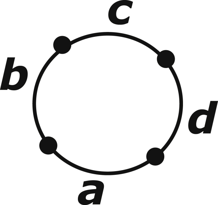
The free energies for forming two-way junctions are shown in Fig. 5. In the topological representation of a two-way junction depicted at the top left of Fig. 5, there are three relevant loop lengths: a is the length of the hairpin loop, b is the length of the junction on the 5′ side, and c is the other junction on the 3′ side. The dangling free ends of the chain are omitted as usual because they do not cost free energy. Fig. 5 shows the additional free energy needed to initiate a two-way junction after the hairpin loop a is in place, as a function of the two junction lengths $b$ and $c$ in nt. Fig. 5 illustrates that the free energy $\mathit{\Delta }G\left(b,c\right)$ is approximately the same when $b$ and $c$ are swapped, indicating that the initiation costs of a two-way junction are roughly symmetric with respect to the 5′ and 3′ junction lengths. The numerical values for $\mathit{\Delta }G\left(b,c\right)$ are tabulated in Table 1, with error estimates given in parentheses. Although a precise comparison between the numerical values obtained from experiments versus simulations is difficult because of the fact that the simulations only accounted for the backbone entropy, the trend observed in our data is nevertheless similar to that from the experiments used in constructing the nearest-neighbor model. The entropic cost in general increases as the size of the loop $(b+c)$ grows and exhibits asymptotic behavior for sufficiently large loop size (21, 22, 48).

Figure 5.

The free-energy costs of forming a two-way junction with 5′ and 3′ junction length $b$ and $c$, respectively, given that a loop $a$ is already in place. (a) The top view is shown. (b) A side view is shown. In general, the free-energy cost grows as the junction size increases and is roughly symmetric when the 5′ and 3′ lengths are swapped. To see this figure in color, go online.

Table 1.

Table of Free-Energy Cost of Forming a Two-Way Junction in kcal/mol as a Function of the 5′ and 3′ Junction Lengths in nt, $b$ and $c$, Respectively

5′ Loop Length (nt), b	3′ Loop Length (nt), c
		0	1	2	3	4	5	6	7
	0	5.22 (0.03)	5.62 (0.04)	6.07 (0.06)	6.16 (0.07)	6.45 (0.09)	6.57 (0.10)	6.53 (0.09)	6.65 (0.11)
	1	5.77 (0.05)	5.98 (0.06)	6.20 (0.07)	6.40 (0.09)	6.47 (0.09)	6.70 (0.11)	6.61 (0.10)	6.72 (0.11)
	2	5.86 (0.05)	6.12 (0.07)	6.27 (0.08)	6.55 (0.10)	6.58 (0.10)	6.75 (0.12)	6.79 (0.12)	6.85 (0.13)
	3	6.11 (0.07)	6.38 (0.08)	6.68 (0.11)	6.62 (0.10)	6.73 (0.11)	6.85 (0.13)	6.92 (0.13)	6.83 (0.12)
	4	6.36 (0.08)	6.48 (0.09)	6.55 (0.10)	7.08 (0.16)	7.18 (0.17)	7.02 (0.15)	7.08 (0.16)	6.85 (0.13)
	5	6.42 (0.09)	6.61 (0.10)	6.55 (0.10)	6.83 (0.12)	6.94 (0.14)	6.79 (0.12)	6.97 (0.14)	6.92 (0.13)
	6	6.47 (0.09)	6.58 (0.10)	6.79 (0.12)	6.87 (0.13)	7.26 (0.18)	6.89 (0.13)	7.05 (0.15)	7.02 (0.15)
	7	6.58 (0.10)	6.42 (0.09)	6.70 (0.11)	6.85 (0.13)	6.81 (0.12)	6.83 (0.12)	6.73 (0.11)	6.77 (0.12)

Error estimates from the simulation are given in parentheses.

Fig. 6 shows how the two-way junction free energy depends on the loop length of the hairpin on the other side of the helix and the length of the stem itself. The conjecture that motivates our topological reduction scheme argues that they should be largely independent. Fig. 6 plots the free energy of initiating a symmetric two-way junction (i.e., $b=c$) as a function of the junction size for a 4 nt hairpin loop with three different stem lengths (1, 4, and 6 nt) as well as a 6 nt hairpin loop with a 1 nt stem and a 7 nt loop with a 1 nt stem. Clearly, the entropic costs for junction formation are independent of the hairpin on the other side of the constraint as well as the helix length. Note that the variation in cost for larger loop sizes is a natural result of the counting experiment. A higher entropic cost corresponds to a smaller number of recorded occurrences, which is more heavily impacted by counting uncertainty. Although not shown explicitly here, the results for all two-way junctions, symmetric or asymmetric, demonstrate similar independence. Error bars are shown explicitly for a few data points to illustrate the size of the typical uncertainties.

Figure 6.

The free-energy cost of forming symmetric two-way junctions plotted for chains with different sizes of the first loop, $a$, and for different lengths of the stem separating $a$ from the two-way junction $(b,c)$. Over the set of three values used for $a$, the free-energy costs to close the junction are consistent with each other. This indicates that the two-way junction is dependent on only the two junction lengths $b$ and $c$, but not the loop on the opposite side $a$. Over the three different stem lengths, the cost to close the symmetric junction shows no discernible dependence on the length of the stem. Typical error bars for selected data points are included. The error for larger loop sizes can be attributed to errors in the counting experiment. The dashed line is a guide for the eye.

Three-way junctions

Three-way junctions are characterized by three different junction lengths, as shown in Fig. 7. As in the case of two-way junctions, the free-energy cost of initiating a three-way junction is largely independent of the hairpins on the opposite side of all three constraints. In Table 2, we tabulate the values of $\mathit{\Delta }G\left(a,b,c\right)$, where $a$ is the length of the 5′ junction, $c$ is the length of the 3′ junction, and $b$ is the length of the junction in the middle; Fig. 8 shows the corresponding free-energy surface. Only one value for $b$ is shown in Table 2; data tables for all other values of $b$ studied are included in the Supporting Materials and Methods. Not surprisingly, closing a three-way junction costs more free energy than two-way junctions, but this additional cost is only marginal. Comparison of our data against experimental results shows some deviations; this is expected, as the introduction of larger loops and more branching helices yields larger contribution to the experimental results from sources that are not included in our simulations, such as sequence-dependent stabilization and coaxial stacking of helices. In terms of comparing against existing simulation results, we observed the same dependence on loop size and number of branching helices as Aalberts and Nandagopal (48). As the loop size increases, the free-energy cost increases. Additionally, as the number of branching helices increases, there is an overall destabilizing effect that increases the cost for all loop sizes (48). This can be seen in the decreased range spanned by the entropy cost as we move from the two-way junction to three- and four-way junctions. The trends are also similar to results obtained in other studies (29, 30), though our predicted entropic costs are somewhat higher. This difference most likely originates from the way in which each simulation handles the torsional motion of the backbone with the other studies using highly discretized models—diamond lattice for Cao and Chen (29) and discrete states configuration space for Zhang et al (30).

figure 7.

Reduced topological representation of the set of constraints defining a three-way junction. For Table 2 and each subtable of Tables S1–S3, the value for b is fixed, whereas a and c change to give rise to the different sizes of the three-way junctions.

Table 2.

Table of Free-Energy Cost of Forming a Three-Way Junction in kcal/mol as a Function of the 5′ and 3′ Junction Length in Nucleotide ($a$ and $c$, Respectively) with the Center Junction Length ($b$) Kept at 1 nt as a Parameter

Center Loop Length b = 1 nt
5′Loop Length (nt), a	3′ Loop Length (nt), c
		0	1	2	3	4	5	6	7
	0	6.54 (0.10)	6.97 (0.15)	7.21 (0.18)	6.84 (0.13)	7.03 (0.16)	7.09 (0.17)	7.34 (0.21)	7.00 (0.15)
	1	6.94 (0.14)	7.06 (0.16)	7.25 (0.19)	7.06 (0.16)	7.25 (0.19)	7.59 (0.27)	7.09 (0.17)	7.30 (0.20)
	2	6.87 (0.13)	6.82 (0.13)	7.03 (0.16)	7.30 (0.20)	7.46 (0.23)	7.30 (0.20)	7.17 (0.18)	7.40 (0.22)
	3	7.25 (0.19)	7.21 (0.18)	7.25 (0.19)	7.34 (0.21)	7.25 (0.19)	7.46 (0.23)	7.40 (0.22)	7.13 (0.17)
	4	7.30 (0.20)	7.30 (0.20)	6.97 (0.15)	7.88 (0.37)	7.46 (0.23)	7.46 (0.23)	7.46 (0.23)	7.59 (0.27)
	5	7.09 (0.17)	7.30 (0.20)	7.59 (0.27)	7.52 (0.25)	7.46 (0.23)	7.34 (0.21)	7.25 (0.19)	7.00 (0.15)
	6	7.34 (0.21)	7.40 (0.22)	7.25 (0.19)	7.40 (0.22)	7.34 (0.21)	7.34 (0.21)	7.30 (0.20)	7.21 (0.18)
	7	6.97 (0.15)	7.09 (0.17)	6.94 (0.14)	7.17 (0.18)	7.06 (0.16)	7.25 (0.19)	7.46 (0.23)	7.13 (0.17)

For $b=0$ and $b\ge 2$, see Tables S1–S3. Error estimates from the simulation are given in parentheses. Entries that have “inf” errors were too infrequently observed during the simulation for errors to be accurately calculated.

Figure 8.

The free-energy costs of forming a three-way junction with 5′ and 3′ junction length $a$ and $c$, respectively, given that junction length $b$ is fixed at 1 nt; this surface corresponds to the data given in Table 2 above. (a) The top view is shown. (b) A side view is shown. To see this figure in color, go online.

Initiation of a third hairpin

Fig. 9 shows the free energy for initiating a third hairpin c after two others (a and b) have been formed, as a function of loop length $c$ in nt. The open circles are the initiation free energy for the first hairpin taken from Fig. 3. The red circles show hairpin initiation on the 5′ side of loop a. The violet squares show hairpin initiation on the 3′ side of loop b, and the green diamonds show hairpin initiation on the strand between a and b. Analogous to the results for the initiation of a second hairpin shown in Fig. 3, the third hairpin is largely independent of the first two. The segment length between any two hairpins in this set of data varies from 0 to 4 nt.

Figure 9.

The free-energy cost of initiating a third hairpin of length $c$ in the presence of two existing loops $(a$ and $b)$. When compared against the cost of initiating a hairpin loop on the free chain, the cost of the third loop is comparable and shows no dependence on the location of the new loop relative to the existing loops. This suggests that the independence of hairpin loops can be extended to any number of loops within a chain. Note that error bars were included for the average cost of the first hairpin, like in Fig. 3; some of them are not visible because of their size. To see this figure in color, go online.

Four-way junctions

Fig. 10 shows the reduced topological representation of a four-way junction, with the loop on the other side of every hairpin having been factored out. The free energy of formation of a four-way junction is a function of the four junction lengths $a$, $b$, $c$, and $d$. Initiation free energies, as an example of a four-way junction, are tabulated in Table 3 for one particular combination of junction lengths $b$ = $c$ = 4 nt. The data shown are the additional free energy costs for the fourth constraint to be met after the first three constraints are in place. To obtain this data set, an ensemble of 2 million MC simulated conformations of (U)₄₂ chains was used. The free energies in Table 3 show that closing a four-way junction generally costs more entropy than a three-way junction (see Table 2), which in turn costs more entropy than two-way junctions. Again, error estimates are given in parentheses. The error bars are a little larger than for the two- and three-way junctions because the probability of observing a four-way junction is quite low. In Table 3, cells that are blank indicate combinations that failed to show up in the 2-million-member MC-simulated ensemble.

Figure 10.

Reduced topological representation of the set of constraints defining a four-way junction. For the purposes of this study, two of the lengths were constrained to be equal and fixed in value $(b=c=4$nt), whereas the other lengths $(a$ and $d)$ were allowed to vary.

Table 3.

Table of Free-Energy Cost of Forming a Four-Way Junction in kcal/mol as a Function of the 5′ and 3′ Junction Length in Nucleotide ($a$ and $d$, Respectively) with the Middle Junction Lengths Fixed ($b=c=4$nt)

Four-Way Junctions with Center Loops with Lengths b = c = 4 nt
5′ Loop Length (nt), a	3′ Loop Length (nt), d
		0	1	2	3	4	5	6	7
	0	7.85 (0.43)	7.85 (0.43)	7.60 (0.32)	8.03 (0.53)	8.27 (0.76)	8.03 (0.53)	–	7.42 (0.27)
	1	7.71 (0.37)	8.03 (0.53)	8.27 (0.76)	8.03 (0.53)	8.27 (0.76)	8.03 (0.53)	–	7.85 (0.43)
	2	8.03 (0.53)	8.03 (0.53)	7.85 (0.43)	8.27 (0.76)	7.71 (0.37)	8.27 (0.76)	7.71 (0.37)	7.60 (0.32)
	3	8.03 (0.53)	7.85 (0.43)	7.85 (0.43)	7.85 (0.43)	–	8.03 (0.53)	7.71 (0.37)	7.85 (0.43)
	4	7.85 (0.43)	7.71 (0.37)	7.85 (0.43)	8.27 (0.76)	7.85 (0.43)	8.27 (0.76)	8.03 (0.53)	7.85 (0.43)
	5	7.71 (0.37)	8.03 (0.53)	7.85 (0.43)	–	7.71 (0.37)	8.03 (0.53)	7.71 (0.37)	7.42 (0.27)
	6	7.71 (0.37)	7.71 (0.37)	8.27 (0.76)	–	7.71 (0.37)	7.60 (0.32)	7.50 (0.29)	7.60 (0.32)
	7	7.50 (0.29)	7.85 (0.43)	7.60 (0.32)	7.42 (0.27)	7.71 (0.37)	8.03 (0.53)	7.85 (0.43)	7.85 (0.43)

Error estimates from the simulation are given in parentheses. Blank entries correspond to events that were not observed during the simulation despite the large size of the ensemble generated.

Discussion

The topological representation we have developed above has been used to aid in the factorization of the joint constraints imposed by typical RNA secondary structure motifs into approximately independent subsets. Here, we discuss the broader application of this scheme.

First, using the topological reduction scheme and the data presented above, calculating the total free-energy cost arising from backbone conformational constraints associated with any structure is simple. Using the three-way junction from Fig. 1 a as an example, we will illustrate this procedure for junction lengths $a$ = 6, $b$ = 4, $c$ = 5, $d$ = 3, and $e$ = 6 nt, with one of the two stems having $f$ basepair steps and the other having $g$. From Fig. 3, the free energy for seeding hairpin loops $d$ = 3 nt and $e$ = 6 nt are 4.8 and 6.6 kcal/mol, respectively. The cost for propagating a seeded hairpin is 5.2 kcal/mol/basepair steps, so the free energy associated with the two stems combined is 5.2 $\times \left(f+g\right)$ kcal/mol. From Table S1 (d), the free energy for a 6-4-5 three-way junction is 7.4 kcal/mol. The total is therefore 18.8 + 5.2$\left(f+g\right)$ kcal/mol.

Topological reduction can also be used to analyze the interdependence of more complex constraints coming from tertiary contacts. An example is shown in Fig. 11. Many riboswitches, such as the guanine-responsive riboswitch from the xpt-pbuX operon of Bacillus subtilis (49) and the thiamine-pyrophosphate-specific riboswitch of Arabidopsis thaliana (50), make use of a three-way junction architecture to form their aptamer domain. When the aptamer binds its target ligand, additional constraints arising from the reconfiguration of the binding pocket either destabilize existing tertiary interactions or stabilize additional tertiary contacts, leading to a rearrangement of the folded structure and causing an upstream or downstream switching sequence to rehybridize and produce a global shape transformation in the riboswitch RNA (51, 52, 53). Fig. 11 shows how some of these interactions renormalize the topology of a three-way junction.

Figure 11.

Diagrammatic representation of the topology of a three-way junction and how it can be altered by the introduction of new tertiary interactions. (a) An unmodified three-way junction, like the one shown in Fig. 1a, is shown. (b) A representation of kissing loops is shown. The new constraint represented by the thick dashed line in the top row of (b) results in a change in connectivity that no longer allows the two loops $\mathit{b}$ and $\mathit{d}$ to be factored. (c) A representation of ligand-mediated base-base contact in the three-way junction is shown. The new constraint closes a portion of the three-way junction into a loop, giving rise to a diagram that is factorizable into four independent subsets corresponding to two hairpins, one two-way junction, and one three-way junction. (d) The kissing loop and ligand-mediated base-base interaction are combined. The effect changes the connectivity to yield a factorizable diagram consisting of a two-way junction and the structure previously seen in (b). (e) The kissing loop interaction is now combined with a triple base interaction. This yields a new structure that is factorizable into a two-way junction and a new multiply-connected loop structure.

The top row of Fig. 11 a shows the same three-way junction architecture from Fig. 1 a without tertiary contacts. The second row in Fig. 11 a shows its topological representation, and the third row shows the final factorized diagram from Fig. 1 a. As described above, without tertiary contacts the two hairpin loops and the junctions are largely independent, and from this, we derive three disjoint sets of constraints. Now consider the addition of a kissing-loop interaction, denoted in Fig. 11 b by a thick dashed line, between hairpins b and d. The topological representation of this structure is shown in the second row of Fig. 11 b, where the constraint imposed by the kissing-loop interaction is represented by a white circle. Because of this extra constraint, this structure is no longer factorizable because it contains no articulation points. Therefore, the kissing-loop interaction modifies the topological structure of the diagram fundamentally. In the language of topology, this diagram now belongs to a different “class” from that of the diagram in Fig. 11 a. This new nonfactorizable topological class is shown on the bottom row of Fig. 11 b.

In Fig. 11 c, a different tertiary interaction is introduced into the three-way junction. The dashed line in the top row of Fig. 11 c denotes a new base-base contact between two of the junctions mediated by a ligand upon binding. The topological representation of this structure is shown in the second row of Fig. 11 c, and complete factorization leads to the diagram on the bottom row of Fig. 11 c. In this case, the two loops b and d corresponding to the hairpins remain factorizable, but the new interaction between loops a and e renormalizes the diagram into a different topological class. The final factorized representation, shown on the bottom row of Fig. 11 c, is topologically equivalent to two hairpin loops, one two-way junction, and one three-way junction.

The structure in Fig. 11 d combines a kissing-loop tertiary contact between b and d with a base-base tertiary interaction between a and e. The final factorized diagram is shown on the bottom row of Fig. 11 d, consisting of one two-way junction plus three multiply-connected loops, which happen to belong to the same topological class as the structure in Fig. 11 b.

Finally, Fig. 11 e introduces a new type of tertiary interaction. The thick three-way dashed line in Fig. 11 e denotes a triple base interaction, such as the one observed in the crystallographic structure of the G-box riboswitch when a guanine is bound into the aptamer domain. The ligand forms contacts simultaneously with three bases, leading to a triplet interaction. Fig. 11 e considers the topological renormalization that is produced by mixing a kissing-loop interaction between hairpins b and d with a base-triple interaction among junctions a, c, and e. The final factorized diagram is shown in the bottom row of Fig. 11 e. This diagram suggests that the structure in Fig. 11 e is topologically equivalent to one two-way junction plus four mutually connected loops. This result also explains how riboswitches based on a three-way junction motif might utilize tertiary interactions coming from ligand binding to induce loop-loop interactions in distal regions of its RNA sequence.

We conclude by mentioning one useful property of factorizable diagrams. After complete factorization, each disjoint piece consists of a self-contained substructure that traces out a close circuit beginning with an initial vertex and ending on the same vertex, traversing every arc inside the substructure once and only once. For each of these substructures, a basic theorem in topology states that the choice of the initial vertex is arbitrary and that the choice of the first arc to follow to start the circuit is also arbitrary. This means that when calculating the entropy of a substructure, the answer does not depend on which constraint (i.e., vertex) is used to start or end. On the other hand, for substructures that do not begin and end on the same vertex, such as the one in Fig. 1 b, they must have exactly two odd vertices. There is only one way to traverse the entire path through such structures, which is to start on one of the odd vertices and end on the other.

The examples here and in the last sections show how our proposed topological perspective of RNA structures could lead to new insights into the interplay among multiple constraints inherent to the secondary and tertiary structures of folded RNAs. Work is currently in progress to generate data for the entropic penalties of a library of tertiary contacts as well as for pseudoknots.

By extending our study to more complex secondary structures, such as those in Fig. 1, c and d, we should be able to examine the validity of the factorization hypothesis in more complex elements and evaluate their entropic costs from simulation. This can then be used to study more complex tertiary folds by mapping the 3D structure to the corresponding 2D graphs, which we can separate into the independent subsets to calculate their entropic costs. Using our atomistic simulations, we can also reconstitute 3D structures from 2D graphs with defined constraints. This would open new ways to study RNA structures within the space of all possible 2D graphs, providing a rigorous strategy to interpolate between 2D and 3D structures and forming the foundation for a large-scale MC simulation algorithm for RNA tertiary structures.

Conclusion

In this article, we take a fresh look at how to interpret the various types of secondary and tertiary structural motifs encountered in typical RNA folds from the point of view of graph theory. We have proposed a diagrammatic scheme to quantify the entropic penalty imposed on the sugar-phosphate backbone of a folded RNA coming from constraints imposed by the secondary and/or tertiary contacts needed to stabilize the fold. Among the various terms in the folding free energy, the free energy coming from entropy depression due to the loss of backbone conformational freedom is the only term that is guaranteed to be always uphill, and as such, it provides a rigorous lower bound on the magnitudes of all the other free-energy contributors that must act to stabilize the fold. Whether folding occurs locally via domains or cooperatively can also be resolved by examining the free-energy balance within each domain against backbone entropic costs.

A simple diagrammatic device is designed to help factor the many secondary and tertiary constraints typically seen in folded RNAs into approximately independent sets to separate the backbone entropy into additive parts. This approach, which to our knowledge is new, generates an interesting and intuitive topological view of RNA structures. We further show how topological reduction can be carried out for typical secondary and tertiary structure motifs, and by comparing the results of the reduction against large-scale MC simulations of equilibrium ensembles of different RNA constructs in solution, we demonstrate the accuracy and usefulness of the topological perspective. Extensive data sets and simple recipes are provided in the article to enable any RNA scientist to easily estimate the magnitude of backbone entropy depression due to common RNA secondary motifs, such as hairpin loops and multiway junctions. Studies quantifying the conformational entropic penalties arising from pseudoknots as well as longer-range tertiary interactions are underway.

Author Contributions

C.H.M. designed the study. C.H.M. and E.N.H.P. carried out the work. C.H.M. wrote the manuscript.

Editor: Tamar Schlick.

References

- 1.Draper D.E., Grilley D., Soto A.M. Ions and RNA folding. Annu. Rev. Biophys. Biomol. Struct. 2005;34:221–243. doi: 10.1146/annurev.biophys.34.040204.144511. [DOI] [PubMed] [Google Scholar]
- 2.Wong G.C., Pollack L. Electrostatics of strongly charged biological polymers: ion-mediated interactions and self-organization in nucleic acids and proteins. Annu. Rev. Phys. Chem. 2010;61:171–189. doi: 10.1146/annurev.physchem.58.032806.104436. [DOI] [PubMed] [Google Scholar]
- 3.Chen S.J. RNA folding: conformational statistics, folding kinetics, and ion electrostatics. Annu. Rev. Biophys. 2008;37:197–214. doi: 10.1146/annurev.biophys.37.032807.125957. [DOI] [PMC free article] [PubMed] [Google Scholar]
- 4.Liu L., Chen S.J. Computing the conformational entropy for RNA folds. J. Chem. Phys. 2010;132:235104. doi: 10.1063/1.3447385. [DOI] [PMC free article] [PubMed] [Google Scholar]
- 5.Woodson S.A. Compact intermediates in RNA folding. Annu. Rev. Biophys. 2010;39:61–77. doi: 10.1146/annurev.biophys.093008.131334. [DOI] [PMC free article] [PubMed] [Google Scholar]
- 6.Turner D.H. Thermodynamics of base pairing. Curr. Opin. Struct. Biol. 1996;6:299–304. doi: 10.1016/s0959-440x(96)80047-9. [DOI] [PubMed] [Google Scholar]
- 7.Chandler D. Oxford University Press; New York: 1987. Introduction to Modern Statistical Mechanics. [Google Scholar]
- 8.Hill T.L. McGraw-Hill; New York: 2013. Statistical Mechanics: Principles and Selected Applications. [Google Scholar]
- 9.Ding F., Sharma S., Dokholyan N.V. Ab initio RNA folding by discrete molecular dynamics: from structure prediction to folding mechanisms. RNA. 2008;14:1164–1173. doi: 10.1261/rna.894608. [DOI] [PMC free article] [PubMed] [Google Scholar]
- 10.Ding F., Lavender C.A., Dokholyan N.V. Three-dimensional RNA structure refinement by hydroxyl radical probing. Nat. Methods. 2012;9:603–608. doi: 10.1038/nmeth.1976. [DOI] [PMC free article] [PubMed] [Google Scholar]
- 11.De Gennes P.-G. Cornell University Press; Ithaca, NY: 1979. Scaling Concepts in Polymer Physics. [Google Scholar]
- 12.Flory P., Volkenstein M. Interscience Publishers; New York: 1969. Statistical Mechanics of Chain Molecules. [Google Scholar]
- 13.Le S.Y., Nussinov R., Maizel J.V. Tree graphs of RNA secondary structures and their comparisons. Comput. Biomed. Res. 1989;22:461–473. doi: 10.1016/0010-4809(89)90039-6. [DOI] [PubMed] [Google Scholar]
- 14.Schmitt W.R., Waterman M.S. Linear trees and RNA secondary structure. Discrete Appl. Math. 1994;51:317–323. [Google Scholar]
- 15.Shapiro B.A., Zhang K.Z. Comparing multiple RNA secondary structures using tree comparisons. Comput. Appl. Biosci. 1990;6:309–318. doi: 10.1093/bioinformatics/6.4.309. [DOI] [PubMed] [Google Scholar]
- 16.Laing C., Schlick T. Computational approaches to RNA structure prediction, analysis, and design. Curr. Opin. Struct. Biol. 2011;21:306–318. doi: 10.1016/j.sbi.2011.03.015. [DOI] [PMC free article] [PubMed] [Google Scholar]
- 17.Kim N., Laing C., Schlick T. Graph-based sampling for approximating global helical topologies of RNA. Proc. Natl. Acad. Sci. USA. 2014;111:4079–4084. doi: 10.1073/pnas.1318893111. [DOI] [PMC free article] [PubMed] [Google Scholar]
- 18.Gan H.H., Fera D., Schlick T. RAG: RNA-As-Graphs database--concepts, analysis, and features. Bioinformatics. 2004;20:1285–1291. doi: 10.1093/bioinformatics/bth084. [DOI] [PubMed] [Google Scholar]
- 19.Fera D., Kim N., Schlick T. RAG: RNA-As-Graphs web resource. BMC Bioinformatics. 2004;5:88. doi: 10.1186/1471-2105-5-88. [DOI] [PMC free article] [PubMed] [Google Scholar]
- 20.Mathews D.H., Sabina J., Turner D.H. Expanded sequence dependence of thermodynamic parameters improves prediction of RNA secondary structure. J. Mol. Biol. 1999;288:911–940. doi: 10.1006/jmbi.1999.2700. [DOI] [PubMed] [Google Scholar]
- 21.Turner D.H., Mathews D.H. NNDB: the nearest neighbor parameter database for predicting stability of nucleic acid secondary structure. Nucleic Acids Res. 2010;38:D280–D282. doi: 10.1093/nar/gkp892. [DOI] [PMC free article] [PubMed] [Google Scholar]
- 22.Mathews D.H., Turner D.H. Prediction of RNA secondary structure by free energy minimization. Curr. Opin. Struct. Biol. 2006;16:270–278. doi: 10.1016/j.sbi.2006.05.010. [DOI] [PubMed] [Google Scholar]
- 23.Diamond J.M., Turner D.H., Mathews D.H. Thermodynamics of three-way multibranch loops in RNA. Biochemistry. 2001;40:6971–6981. doi: 10.1021/bi0029548. [DOI] [PubMed] [Google Scholar]
- 24.Zuker M. Computer prediction of RNA structure. Methods Enzymol. 1989;180:262–288. doi: 10.1016/0076-6879(89)80106-5. [DOI] [PubMed] [Google Scholar]
- 25.Zuker M., Mathews D.H., Turner D.H. Algorithms and thermodynamics for RNA secondary structure prediction: a practical guide. In: Barciszewski J., Clark B.F.C., editors. RNA Biochemistry and Biotechnology. Springer; 1999. pp. 11–43. [Google Scholar]
- 26.Zuker M. Mfold web server for nucleic acid folding and hybridization prediction. Nucleic Acids Res. 2003;31:3406–3415. doi: 10.1093/nar/gkg595. [DOI] [PMC free article] [PubMed] [Google Scholar]
- 27.Zuker M. On finding all suboptimal foldings of an RNA molecule. Science. 1989;244:48–52. doi: 10.1126/science.2468181. [DOI] [PubMed] [Google Scholar]
- 28.Zadeh J.N., Steenberg C.D., Pierce N.A. NUPACK: analysis and design of nucleic acid systems. J. Comput. Chem. 2011;32:170–173. doi: 10.1002/jcc.21596. [DOI] [PubMed] [Google Scholar]
- 29.Cao S., Chen S.J. Predicting RNA folding thermodynamics with a reduced chain representation model. RNA. 2005;11:1884–1897. doi: 10.1261/rna.2109105. [DOI] [PMC free article] [PubMed] [Google Scholar]
- 30.Zhang J., Lin M., Liang J. Discrete state model and accurate estimation of loop entropy of RNA secondary structures. J. Chem. Phys. 2008;128:125107. doi: 10.1063/1.2895050. [DOI] [PMC free article] [PubMed] [Google Scholar]
- 31.Arnold B.H. Dover Publications; Mineola, NY: 2011. Intuitive Concepts in Elementary Topology. [Google Scholar]
- 32.Balakrishnan R., Ranganathan K. Springer Science & Business Media; New York: 2012. A Textbook of Graph Theory. [Google Scholar]
- 33.Mak C.H. Atomistic free energy model for nucleic acids: simulations of single-stranded DNA and the entropy landscape of RNA stem-loop structures. J. Phys. Chem. B. 2015;119:14840–14856. doi: 10.1021/acs.jpcb.5b08077. [DOI] [PubMed] [Google Scholar]
- 34.Mak C.H., Sani L.L., Villa A.N. Residual conformational entropies on the sugar-phosphate backbone of nucleic acids: an analysis of the nucleosome core DNA and the ribosome. J. Phys. Chem. B. 2015;119:10434–10447. doi: 10.1021/acs.jpcb.5b04839. [DOI] [PubMed] [Google Scholar]
- 35.Mak C.H., Matossian T., Chung W.Y. Conformational entropy of the RNA phosphate backbone and its contribution to the folding free energy. Biophys. J. 2014;106:1497–1507. doi: 10.1016/j.bpj.2014.02.015. [DOI] [PMC free article] [PubMed] [Google Scholar]
- 36.Mak C.H., Chung W.Y., Markovskiy N.D. RNA conformational sampling: II. Arbitrary length multinucleotide loop closure. J. Chem. Theory Comput. 2011;7:1198–1207. doi: 10.1021/ct100681j. [DOI] [PubMed] [Google Scholar]
- 37.Mak C.H. RNA conformational sampling. I. Single-nucleotide loop closure. J. Comput. Chem. 2008;29:926–933. doi: 10.1002/jcc.20851. [DOI] [PubMed] [Google Scholar]
- 38.Weeks J.D., Chandler D., Andersen H.C. Role of repulsive forces in determining the equilibrium structure of simple liquids. J. Chem. Phys. 1971;54:5237–5247. [Google Scholar]
- 39.Henke P.S., Mak C.H. Free energy of RNA-counterion interactions in a tight-binding model computed by a discrete space mapping. J. Chem. Phys. 2014;141:064116. doi: 10.1063/1.4892059. [DOI] [PubMed] [Google Scholar]
- 40.Mak C.H., Henke P.S. Ions and RNAs: free energies of counterion-mediated RNA fold stabilities. J. Chem. Theory Comput. 2013;9:621–639. doi: 10.1021/ct300760y. [DOI] [PubMed] [Google Scholar]
- 41.Mak C.H. Unraveling base stacking driving forces in DNA. J. Phys. Chem. B. 2016;120:6010–6020. doi: 10.1021/acs.jpcb.6b01934. [DOI] [PubMed] [Google Scholar]
- 42.Rury A.S., Ferry C., Mak C.H. Solvent thermodynamic driving force controls stacking interactions between polyaromatics. J. Phys. Chem. C. 2016;120:23858–23869. [Google Scholar]
- 43.Hummer G., Garde S., Pratt L.R. An information theory model of hydrophobic interactions. Proc. Natl. Acad. Sci. USA. 1996;93:8951–8955. doi: 10.1073/pnas.93.17.8951. [DOI] [PMC free article] [PubMed] [Google Scholar]
- 44.Henke P.S., Mak C.H. An implicit divalent counterion force field for RNA molecular dynamics. J. Chem. Phys. 2016;144:105104. doi: 10.1063/1.4943387. [DOI] [PubMed] [Google Scholar]
- 45.Coimbatore Narayanan B., Westbrook J., Berman H.M. The nucleic acid database: new features and capabilities. Nucleic Acids Res. 2014;42:D114–D122. doi: 10.1093/nar/gkt980. [DOI] [PMC free article] [PubMed] [Google Scholar]
- 46.Berman H.M., Olson W.K., Schneider B. The nucleic acid database. A comprehensive relational database of three-dimensional structures of nucleic acids. Biophys. J. 1992;63:751–759. doi: 10.1016/S0006-3495(92)81649-1. [DOI] [PMC free article] [PubMed] [Google Scholar]
- 47.Serra M.J., Turner D.H. Predicting thermodynamic properties of RNA. Methods Enzymol. 1995;259:242–261. doi: 10.1016/0076-6879(95)59047-1. [DOI] [PubMed] [Google Scholar]
- 48.Aalberts D.P., Nandagopal N. A two-length-scale polymer theory for RNA loop free energies and helix stacking. RNA. 2010;16:1350–1355. doi: 10.1261/rna.1831710. [DOI] [PMC free article] [PubMed] [Google Scholar]
- 49.Batey R.T., Gilbert S.D., Montange R.K. Structure of a natural guanine-responsive riboswitch complexed with the metabolite hypoxanthine. Nature. 2004;432:411–415. doi: 10.1038/nature03037. [DOI] [PubMed] [Google Scholar]
- 50.Thore S., Leibundgut M., Ban N. Structure of the eukaryotic thiamine pyrophosphate riboswitch with its regulatory ligand. Science. 2006;312:1208–1211. doi: 10.1126/science.1128451. [DOI] [PubMed] [Google Scholar]
- 51.Manzourolajdad A., Arnold J. Secondary structural entropy in RNA switch (Riboswitch) identification. BMC Bioinformatics. 2015;16:133. doi: 10.1186/s12859-015-0523-2. [DOI] [PMC free article] [PubMed] [Google Scholar]
- 52.Roth A., Breaker R.R. The structural and functional diversity of metabolite-binding riboswitches. Annu. Rev. Biochem. 2009;78:305–334. doi: 10.1146/annurev.biochem.78.070507.135656. [DOI] [PMC free article] [PubMed] [Google Scholar]
- 53.Montange R.K., Batey R.T. Riboswitches: emerging themes in RNA structure and function. Annu. Rev. Biophys. 2008;37:117–133. doi: 10.1146/annurev.biophys.37.032807.130000. [DOI] [PubMed] [Google Scholar]
Associated Data
This section collects any data citations, data availability statements, or supplementary materials included in this article.