A theoretical and non-destructive experimental approach for direct inclusion of measured collagen orientation and recruitment into mechanical models of the artery wall

Abstract

Gradual collagen recruitment has been hypothesized as the underlying mechanism for the mechanical stiffening with increasing stress in arteries. In this work, we investigated this hypothesis in eight rabbit carotid arteries by directly measuring the distribution of collagen recruitment stretch under increasing circumferential loading using a custom uniaxial (UA) extension device combined with a multi-photon microscope (MPM). This approach allowed simultaneous mechanical testing and imaging of collagen fibers without traditional destructive fixation methods. Fiber recruitment was quantified from 3D rendered MPM images, and fiber orientation was measured in projected stacks of images. Collagen recruitment was observed to initiate at a finite strain, corresponding to a sharp increase in the measured mechanical stiffness, confirming the previous hypothesis and motivating the development of a new constitutive model to capture this response.

Previous constitutive equations for the arterial wall have modeled the collagen contribution with either abrupt recruitment at zero strain, abrupt recruitment at finite strain or as gradual recruitment beginning at infinitesimal strain. Based our experimental data, a new combined constitutive model was presented in which fiber recruitment begins at a finite strain with activation strain represented by a probability distribution function. By directly including this recruitment data, the collagen contribution could be modeled using a simple Neo-Hookean equation. As a result, only two phenomenological material constants needed to be fit from the stress stretch data. Three other models for the arterial wall were then compared with these results. The approach taken here was successful in combining stress-strain analysis with simultaneous microstructural imaging of collagen recruitment and orientation, providing a new approach by which underlying fiber architecture may be quantified and included in constitutive equations.

1. Introduction

The healthy artery wall is a layered composite material and often assumed to consist of an isotropic mechanism arising from components of extracellular matrix (ECM) and and one or more anisotropic mechanisms due to “fabric-like” embedded collagen fibers. At low loads the passive mechanical response is assumed to be dominated by the isotropic ECM contribution. The crimped circumferentially-oriented medial collagen fibers are hypothesized to gradually unfurl and begin load bearing under increasing pressure (Burton, 1954; Roach and Burton, 1957; Scott et al., 1972).

While it is commonly stated that collagen begins load bearing at finite strain, only a few constitutive equations include this behavior. Abrupt fiber recruitment beginning at finite strain is considered in a previous model of the artery wall (Wulandana and Robertson, 1999, 2005; Watton et al., 2009), which has been extended to include anisotropic, structurally motivated models for collagen (Li and Robertson, 2009a) as well as subfailure damage of elastin and collagen Li and Robertson (2009b); Robertson et al. (2011). This behavior can play an important role in cases where the isotropic contribution of the ECM is damaged, for example in balloon angioplasty or fatigue damage, (e.g. Robertson et al. (2011)). However, challenges in observing collagen unfurling in a single specimen have limited the direct measurement of this process In conventional histological approaches, the arterial wall is fixed and collagen is stained at various stretch levels prior to analysis. Numerous samples are needed to obtain collagen data at different levels of stretch (e.g. Roy et al. (2010)). However, due to issues of interspecimen variability it is difficult, if not impossible, to directly evaluate the recruitment initiation process using compiled data of this kind.

Multi-photon microscopy provides an opportunity to exploit second harmonic generation (SHG) to evaluate collagen structure without staining or fixation. SHG takes place when the electric field from exciting light deforms a non-symmetrical molecule, creating an oscillating field at twice the frequency, the second harmonic (Taatjes and Mossman, 2006). Arterial collagen can be imaged due to its non-symmetrical triple helix arrangement. Biomechanical devices may be used in conjunction with multi-photon microscopy (MPM) to visualize elastin and collagen structure in segments of arterial wall under various loading conditions without staining (Megens et al., 2007; Zoumi et al., 2004; Arkill et al., 2010; Hill and Robertson, 2010). Arterial collagen may also be imaged using SHG in a confocal system (Wan et al., 2010).

We recently developed a system for combined uniaxial testing (UA) and multi-photon microscopy measurement of the mechanical response with nondestructive imaging of collagen and elastin and used this system to assess damage to the internal elastic lamainae in human cerebral arteries (Hill and Robertson, 2010; Robertson et al., 2011).

In the current work, the UA-MPM system was used to evaluate the mechanical and microstructural recruitment of medial collagen fibers in the common carotid artery of New Zealand white rabbits. Collagen recruitment and fiber orientation were directly assessed from UA-MPM studies of circumferentially loaded tissue samples. Distribution of fiber tortuosity was evaluated from three dimensional reconstructed segments. Fibers were defined as recruited when the tortuosity decreased below a critical level. Collagen fiber orientation was measured using derivative information calculated with the standard Sobel-kernel filter (Elbischger, 2005; Chaudhuri et al., 1993; Karlon et al., 1998) that has previously been used to determine the distribution of fiber angle in tissue-engineered scaffolds (Courtney et al., 2006).

Based on experimental results obtained with this device, a new structurally motivated strain energy function for the artery wall was developed. The model presented here was strongly motivated by the early work of Lanir (1979, 1983) as well as more recent work by Sacks (2000). Lanir originally formulated a three-dimensional structural model of the artery wall that directly includes the distribution of both collagen fiber orientation and recruitment Lanir (1979, 1983). The measured biaxial mechanical response and distribution of fiber orientation from small angle light scattering of heart valve tissue (Sacks et al., 1997; Sacks, 2000) has been directly incorporated into Lanir’s structural model (Sacks, 2003), with the parameters of the gradual recruitment probability distribution function (PDF) obtained from a least-squares fit. Recently, collagen fiber recruitment has been quantified in rabbit carotid arteries using staining and fixation with confocal microscopy (Roy et al., 2010). Collagen fiber recruitment was assumed to initiate at an infinitesimal strain, with subsequent fiber engagement represented by a PDF.

In this current work, a model is presented in which fiber recruitment begins at finite strain with gradual recruitment stretches modeled using a PDF. The measured structural and mechanical data taken with the UA-MPM system are directly incorporated into this constitutive model. For comparison, the data are also used to assess three other constitutive models with different levels of structural content. Elasticity constants are obtained from a non-linear regression analysis of the mechanical loading data. The utility of each model is discussed.

2. Constitutive Model for the Arterial Wall

The total mechanical response of the arterial wall is modeled as incompressible, arising from an additive combination of isotropic and anisotropic hyperelastic components, with total strain energy per unit volume in reference configuration κ₀,

$$W=W_{\mathit{iso}}+W_{\mathit{aniso}}.$$ (1)

2.1. Isotropic Mechanism

The strain energy potential of the isotropic mechanism is given as a function of the deformation gradient relative to κ₀ (Fig. 1), denoted as F. After imposing invariance requirements, the incompressibility condition, and material isotropy, this strain energy potential can be expressed without loss in generality in terms of the first and second principal invariants of C = F^TF (equivalent to those of b = FF^T):

$$W_{\mathit{iso}}=W_{\mathit{iso}}(I,II)$$ (2)

where I = tr(C), II = (1/2)[tr(C²) − (trC)²].

Figure 1.

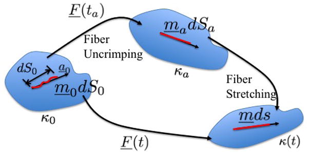
Schematic of reference configurations and notation used for fiber recruitment kinematics.

2.2. Anisotropic Mechanism

The anisotropic mechanism is modeled as arising from the fibrous architecture of the artery wall. In formulating the constitutive response, a single fiber is considered in a representative volume element (RVE) at an arbitrary material point in the body. In a given RVE, collagen fibers display a distribution of fiber waviness and are therefore recruited to load bearing over a range of stretch values. In general, a range of collagen fiber orientations will also be found in each RVE. In the following subsections, the kinematics employed for fiber recruitment and the functional representations for the distributions of fiber orientation and recruitment are described.

2.2.1. Kinematics of fiber recruitment

The configuration in which a fiber is recruited to load bearing (activated) is denoted as κ_a and a unit vector m_a denotes its direction in κ_a at some time t_a, Fig. 1. Under an affine transformation, an infinitesimal material element m_a dS can be mapped back to a material element dm₀ S₀ in κ₀, where m₀ is also a unit vector. These material elements can be related through,

$${\mathbf{m}}_a{dS}_a=\mathbf{F}(t_a){\mathbf{m}}_0{dS}_0.$$ (3)

The activation stretch is defined as λ_a = dS_a/dS₀. If the same fiber segment undergoes further stretch and rotation, so that at arbitrary current time t, it has orientation m and length ds, it can similarly be mapped back to κ₀ through,

$$\mathbf{m}ds=\mathbf{F}(t){\mathbf{m}}_0{dS}_0.$$ (4)

Defining λ_f = ds/dS₀ and the “true” fiber stretch, or stretch after uncrimping, as λ_t = ds/dS_a, it then follows that

$${\lambda }_t={\lambda }_f/{\lambda }_a.$$ (5)

The stretch λ_f can be obtained using Eq. 4,

$${\lambda }_f^2=\mathbf{C}(t):({\mathbf{m}}_0\otimes {\mathbf{m}}_0).$$ (6)

The distribution of λ_a for an arbitrary RVE will be treated as a material property of the fiber reinforced material and measured directly from the MPM images. As discussed below, the mechanical response of the collagen fibers depends only on the deformation of collagen relative to the reference configuration κ_a, not on κ₀. Therefore, the geometric configuration of the buckled fiber in κ₀ is not important in the model. Instead, as detailed below, the distribution of critical stretches required for recruitment is directly measured.

2.2.2. Distribution of fiber orientation

In general, a distribution of fiber orientations will exist in the RVE. For convenience, we define the distribution after it is mapped back to κ₀ using an orientation density function ρ = ρ(m_o), (e.g. Gasser et al. (2006); Lanir (1994)).

Using local rectilinear coordinates with unit base vectors (e₁, e₂, e₃) (Fig. 2a), the vector m₀ can be written with respect to spherical coordinates θ and φ, through

Figure 2.

Schematic displaying the geometric variables used in modelling the distribution of collagen fiber orientation for (a) general 3D distribution and (b) planar or “fan splay” distribution.

$${\mathbf{m}}_0(\theta ,\phi )=cos\theta {\mathbf{e}}_1+sin\theta cos\phi {\mathbf{e}}_2+sin\theta sin\phi {\mathbf{e}}_3.$$ (7)

Hence, the orientation density function can be written as a function of θ ∈ [−π/2, π/2] and φ ∈ [0, π], (Fig. 2a). Note that each fiber is only counted once, since for an arbitrary m₀, the fiber −m₀ is not included.

The distribution function is non-negative and defined such that ρ(θ, φ) cos θ dθ dφ represents the proportion of fibers with angles in the range [θ, θ + dθ] and [φ, φ + dφ] where ρ(θ, φ) is taken to be normalized on a unit semi-sphere,

$$1=\frac{1}{2\pi }{\int }_0^{\pi }{\int }_{-\pi /2}^{\pi /2}\rho (\theta ,\phi )cos\theta d\theta d\phi .$$ (8)

A special case of this 3D distribution is planar splay, for which the distribution of fibers in an RVE lies within a single plane, (e.g. Freed (2008); Freed et al. (2005)). In this case, a local rectilinear basis may be chosen such that all fibers lie within the e₁ ⊗ e₂ plane (Fig. 2b). A 2D orientation distribution function ρ_2D(θ) can then be defined on θ ∈ [−π/2, π/2] with normalization condition,

$$1=\frac{1}{\pi }{\int }_{-\pi /2}^{\pi /2}{\rho }_{2D}(\theta )d\theta .$$ (9)

Following the approach of Lanir (1994), the strain energy function for the material is then the result of the integrated response of fibers over all angles,

$$W_{\mathit{aniso}}=\frac{1}{\pi }{\int }_{-\pi /2}^{\pi /2}{w}_f({\lambda }_f^2){\rho }_{2D}(\theta )d\theta .$$ (10)

As described in the next section, measurements of fiber orientation distribution will be made in configurations where the fibers are largely recruited to avoid experimental artifacts arising from fiber crimp. This distribution of orientation can then be mapped or “pulled” back to reference configuration κ₀ using Eq. 4, to obtain ρ_2D(θ).

2.2.3. Distribution of fiber recruitment

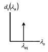
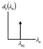
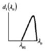
As in Lanir (1979), it is assumed that collagen fibers are unable to bear load until they are “straightened”. The strain energy function of a fiber is therefore modeled as a function of the stretch (λ_t) beyond the critical straightening or “activation” stretch, λ_a. From Eq. 5, λ_t = λ_f/λ_a and λ_f can be determined from Eq. 6. In general, the collagen fibers in an RVE will require a distribution of fiber activation stretches, a material property of the material. Lanir (1994) modeled this distribution using a recruitment probability distribution function (PDF), which is represented here as d₁(λ_a). For the range of stretch [λ_a, λ_a + dλ_a], the fraction of fibers of a given orientation in RVE that became straight are represented by d₁(λ_a)dλ_a. The contribution to the strain energy from this fiber ensemble is $d_1({\lambda }_a)w_f^{\ast }({\lambda }_t)d{\lambda }_a$. Therefore, the strain energy potential of the whole fiber ensemble in the RVE for the esemble is

$$w_f({\lambda }_f^2)={\int }_1^{{\lambda }_f}{d}_1({\lambda }_a)w_f^{\ast }\left(\frac{{\lambda }_f^2}{{\lambda }_a^2}\right)d{\lambda }_a.$$ (11)

The collagen fibers in an RVE are assumed to bear no load when the local tissue stretch is less than the minimum recruitment stretch, λ_a1. Here, this condition is directly imposed by defining d₁(λ_a) to be zero for λ_a ≤ λ_a1. It can also be imposed using a Heaviside function (Robertson et al., 2011).

2.3. Choice of material functions

Four anisotropic models with a range of simplifying assumptions for collagen recruitment are considered and compared (Table 1), with Model D being the most general. The recruitment process is depicted graphically in Table 1 using the disconnecting hook schematic of Wiederhielm (1965); Barra et al. (1993).

Table 1.

Four forms of the anisotropic strain energy function considered

Model	Model A	Model B	Model C	Model D
	Fiber strain energy
$W_f^{\ast }({\lambda }_t^2)$	$=\frac{\eta }{\gamma }[e^{\gamma ({\lambda }_t^2-1)}-1]$	$=\frac{\eta }{\gamma }[e^{\gamma ({\lambda }_t^2-1)}-1]$	$=\frac{\eta }{2}({\lambda }_t^2-1)$	$=\frac{\eta }{2}({\lambda }_t^2-1)$
	Fiber recruitment
	Abrupt commences at λ > 1	Abrupt commences at λ > 1	Gradual commences at λ = 1	Gradual commences at λ ≥ 1
d1(λa)	= δ[λ–λa1]	= δ[λ–λa1]	$=\{\begin{array}{ll}{\mathrm{\Gamma }}_{\mathit{PDF}}\hfill & {\lambda }_a\ge 1\hfill \\ 0\hfill & {\lambda }_a<1\hfill \end{array}$	$=\{\begin{array}{ll}{\mathrm{\Gamma }}_{\mathit{PDF}}\hfill & {\lambda }_a\ge {\lambda }_{a1}\hfill \\ 0\hfill & {\lambda }_a<{\lambda }_{a1}\hfill \end{array}$
	Fiber orientation
ρ2D(θ)	= πδ[θ]	General	General	General

In all four models, the isotropic mechanism is represented as a single spring that engages immediately upon loading. For simplicity, and motivated by earlier work, a neo-Hookean model is used for the isotropic response for all models, (Watton et al., 2009; Valentin et al., 2009; Humphrey and Rajagopal, 2003; Humphrey, 1999; Dorrington and McCrum, 1977),

$$W_{\mathit{iso}}=\frac{{\eta }_0}{2}(I-3),{\mathit{\sigma }}_{\mathit{iso}}={\eta }_0\mathbf{b}.$$ (12)

Collagen fibers are represented by a collection of springs that engage at various levels of tissue extension. All fibers are engaged once a critical stretch value is reached, modeled by defining as d₁(λ_α) as a generalized function known as the Dirac delta function.

In gradual recruitment (Models C and D), fibers in the RVE require a range of recruitment stretches to be activated. A probability density function for the gamma distribution (Γ_PDF ) was used to model recruitment in these models,

$$d_1({\lambda }_a)=\{\begin{array}{ll}0\hfill & \text{for}{\lambda }_a<{\lambda }_{a1}\hfill \\ {\mathrm{\Gamma }}_{\mathit{PDF}}({\lambda }_a-{\lambda }_{a1})\hfill & \text{for}{\lambda }_a\ge {\lambda }_{a1}\hfill \end{array}$$ (13)

where

$${\mathrm{\Gamma }}_{\mathit{PDF}(x;\alpha ,\beta )}=x^{\alpha -1}{e}^{-x/\beta }\frac{1}{{\beta }^{\alpha }\mathrm{\Gamma }(\alpha )}x\ge 0,\alpha ,\beta >0$$ (14)

and α is the shape parameter, β is the scale parameter and Γ(·) the Gamma function. Eq. 14 is similar to that used by Sacks (2003), though it is generalized to include a non-zero location parameter λ_a1 so that collagen recruitment can be modeled as initiating at finite strain. Zulliger et al. (2004) introduced a log logistic distribution for collagen recruitment and the model was further developed by Roy et al. (2010). These authors also considered recruitment to begin at zero strain. To demonstrate this approach, recruitment in Model C is modeled as commencing immediately (λ_a1 = 1). This approach is generalized in Model D to include commencement of recruitment at finite strain (λ_a1 ≥ 1), displayed schematically in Table 1, by the delayed involvement of the first collagen spring in Models A, B and D.

Motivated by results obtained by Li and Robertson (2009a,b), an exponential strain energy function was used in the abrupt recruitment models,

$$w_f^{\ast }=\frac{\eta }{\gamma }\left[e^{\gamma ({\lambda }_t^2-1)}-1\right],$$ (15)

while for both Models C and D, the following simple dependence on λ_t was used,

$$w_f^{\ast }=\frac{\eta }{2}({\lambda }_t^2-1).$$ (16)

As further justified in the results section, the collagen distribution in all models was idealized as planar with orientation distribution function ρ_2D(θ) measured directly from MPM images. The only exception was Model A, in which collagen fiber alignment was assumed to lie completely in the circumferential direction. The total strain energy for the fibers can be obtained from Eqs. 10 and 11 and used to calculate the total anisotropic contribution to the Cauchy stress tensor (e.g. Robertson et al. (2011)),

$${\mathit{\sigma }}_{\mathit{aniso}}=\mathbf{F}\left[\frac{2}{\pi }{\int }_{-\pi /2}^{\pi /2}{\rho }_{2D}(\theta )\frac{{dw}_f({\lambda }_f^2)}{d{\lambda }_f^2}{\mathbf{m}}_0\otimes {\mathbf{m}}_{0}d\theta \right]{\mathbf{F}}^T$$ (17)

where it follows from Eq. 11 that

$$\frac{{dw}_f({\lambda }_f^2)}{d{\lambda }_f^2}={\int }_1^{{\lambda }_f}{d}_1({\lambda }_a)\frac{1}{{\lambda }_a^2}\frac{{dw}_f^{\ast }({\lambda }_t^2)}{d{\lambda }_t^2}d{\lambda }_a,$$ (18)

and therefore the total Cauchy stress σ can be calculated from

$$\mathit{\sigma }={\mathit{\sigma }}_{\mathit{iso}}+{\mathit{\sigma }}_{\mathit{aniso}}$$ (19)

using Eqs. 12 and 17.

3. Methods

A uniaxial (UA) mechanical testing device was constructed to operate in conjunction with a multi-photon microscope for coincident stress-strain analysis and laser scanning imaging of collagen, (Robertson et al., 2011). This horizontal UA device mounted directly underneath the MPM objective lens, so the lens could be lowered for vessel imaging during mechanical experimentation. Mechanical testing and imaging were performed with this UA-MPM system.

3.1. Tissue Samples

Samples (n=8) of left and right rabbit carotid arteries were obtained from New Zealand white rabbits, average weight 4.7 ± 0.008 kg, sacrificed for other studies that did not interfere with the carotid arteries or the circulation. A sample of artery tissue was removed from its source, opened longitudinally, manually cut into a “dogbone” shape, so the long axis of the strip was oriented along the circumference of the vessel. Thickness (H) and width (w) were measured five times with calipers and averaged.

3.2. Mechanical Testing

The mechanical data were obtained with the UA-MPM system, with the illustrated method presented in the first column of Fig. 3. The tissue strips were loaded in the device within a bath of 0.9%w/v saline, (Fig. 3, top row, left). The intimal side of the tissue was loaded facing the MPM lens and oriented for extension in the circumferential direction. The loading direction x₁ (Fig. 2b), corresponded to the circumferential direction of the vessel, the direction x₂ with the axial (blood flow) direction, and x₃ with the radial direction through the thickness of the vessel wall.

Figure 3.

Illustration of the methodology used to determine model parameters. Top row, left to right: specimen of carotid artery between the clamps of the UA-MPM device, illustration of collagen recruitment analysis, depiction of collagen orientation analysis. Middle row, left to right: raw stress-stretch results from testing, tortuosity data and the Gamma cumulative distribution function plotted against stretch, orientation distribution histogram. Bottom: final results from UA-MPM testing of a rabbit carotid artery. Raw stress-stretch data (blue dots) and structural model fit (blue line) from uniaxial tension tests in the circumferential direction with overlaid recruitment probability distribution function (green line).

The tissue was subjected to uniaxial extension with a triangular displacement curve, at 19μm per second. Force and displacement were recorded from the last cycle, post pre-conditioning of at least 5 cycles. The tissue was exposed to increasing displacements until about 1N of maximum force was recorded after preconditioning. Displacement of the clamps was used for strain measurement. First Piola (engineering) stress was computed by dividing force by the original cross sectional area, with area calculated as specimen width multiplied by wall thickness. First Piola Stress was converted to Cauchy stress (per unit area of the deformed configuration) assuming an isochoric deformation and used to obtain curves of stress versus tissue stretch, σ₁₁(λ₁), (Fig. 3, middle row, left). Following uniaxial testing, the tissue was extended and held at 6 levels of (increasing) stretch for MPM imaging.

3.3. Collagen Fiber Imaging

Specimens were extended and MPM imaged at 6 different stretches using an Olympus FV1000 MPE (Tokyo, Japan) equipped with a Spectra-Physics DeepSee Mai Tai Ti-Sapphire laser (Newport, Mountain View, CA). The SHG signals were collected using backscattered epi-detectors. These detectors were non-descanned. An excitation wavelength of 870nm and 1.12NA 25x MPE water immersion objective were used for all samples. The SHG signal was collected using a 400nm emission filter with a ± 50 spectral bin. All filters were provided by Chroma (Brattleboro, VT). The dwell time was 10 microseconds/pixel at a scan pixel count of 1024 X 1024.

Resolution of 0.12μm was achieved with this system. Planar images of the media were initially taken near the adventitia, and subsequent image stacks were taken in 0.5μm intervals moving in the e₃ direction, upward toward the intima. During the approximately 30 minutes of image acquisition for each stretch level, the tissue extension was held fixed. The entire thickness of the vessel wall was captured with this technique, as illustrated by a through-thickness cross section of the 3D reconstructed wall, Fig. 4.

Figure 4.

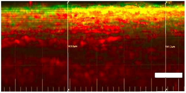
Planar slice from 3D reconstructed unloaded artery. Circumferential direction is left to right and radial direction is up and down with lumen side at top. Moving down from lumen side, the media with layered crimped collagen fibers (red) and elastin fibers can be seen. Below this is the loose, wavy adventitial collagen. Bar = 50μm

3.3.1. Fiber Recruitment Analysis: d₁(λ_a)

Collagen fiber recruitment was measured and incorporated into the constitutive response, with the illustrated method presented in the second column of Fig. 3. Collagen uncrimping was quantified through fiber tortuosity, a measure of the waviness of the collagen fiber, defined as the ratio of fiber arc length to cord length, τ = s/l. Fiber arc length (s) was measured in 3D reconstructed images using a fast marching algorithm for fiber tracing that is a generalization of the 2D method described in Meijering et al. (2004). This algorithm was implemented using the automated Filament function in Imaris (Bitplane, Switzerland). Starting and ending points were specified by the operator. Cord length (l) was defined as the length of a best fit line to the same segment. For illustration, fiber tracings for a representative 3D reconstructed subregion are shown in white in Fig. 3 (top row, middle) in a projected 2D snapshot. A collagen fiber was defined as recruited when its tortuosity decreased below 1.02. Tortuosity was determined for 20 fibers per image and the percentage of recruited fibers at each stretch was computed. To reduce user bias, the operator was blinded to the measured stretch for the images.

The critical stretch at which recruitment initiated (λ_a1) was defined as the lowest stretch at which at least one fiber was recruited. Recruitment parameters α and β were obtained by fitting the Gamma cumulative distribution function (CDF) for the gamma probability distribution function (PDF), given in Eq. 13 by Eq. 14, to the data using the Levenberg-Marquardt nonlinear least squares method.

We evaluated the sensitivity of average tortuosity to fiber number by comparing results for 15, 17 and 20 fiber studies. The values for average tortuosity using 17 and 15 fibers were within 0.4% and 1.0% of the value for 20 fibers, respectively.

3.3.2. Fiber Orientation Analysis: ρ(θ)

Collagen fiber orientation distribution was measured and incorporated into the constitutive response, with the illustrated method presented in the third column of Fig. 3. Fiber orientation was measured on 2D images formed from superimposed projections of the 3D MPM stacks on the e₁ ⊗ e₂ plane. As detailed below, direction vectors for collagen fibers in a subregion were determined using an edge detection algorithm. For illustration, direction vectors are shown for a representative small subregion, in Fig. 3 (top row, right). The fiber angles obtained from the 3D stacks were used to calculate a histogram of weighted fiber angles, shown in blue in Fig. 3 (middle row, right). Angle θ = 0° corresponds to fibers aligned with e₁ (circumferentially aligned) and θ = 90° and −90° correspond to those aligned with e₂ and −e₂, respectively. Ordinate values indicate normalized probability and abscissa values indicate orientation in radians.

The collagen fiber orientation was measured using a previously developed method (Chaudhuri et al., 1993) that has been applied to biological tissues (Karlon et al., 1998; Courtney et al., 2006). Superimposed grayscale MPM images of collagen fibers were imported into a custom MATLAB program. Three points were selected and averaged to determine background intensity. Grayscale values falling below this level were disregarded. Briefly, fiber edge detection was performed by convolving two masks of a selected size (7 × 7 pixels), one horizontal and the other vertical, with the image at each pixel, to give gradient measures Gx and Gy, respectively. The vector containing the sum of the squares of the convolved horizontal and vertical gradient measures was used as a weighting function (G = Gx² +Gy²), while the direction at each pixel was computed as the inverse tangent of the gradient measures (tan⁻¹Gx/Gy). The histogram for direction vector calculation was constructed by defining a subregion with a given size (4 × 4 pixels) and computing the direction associated with the highest weighted value in the subregion. A weighted accumulator function (see Chaudhuri et al. (1993); Courtney et al. (2006) for specific details) was implemented over this subregion, and the summed gradient-weighted contribution of each pixel was determined for each angle on the domain [−90°, 90°] at 1° increments. The dominant orientation was identified as the maximum accumulator bin value within a sub-region, and values representing each bin were accumulated in a histogram to define the collagen fiber dispersion.

For all specimens, the collagen orientation probability distribution data were evaluated at maximum stretch to avoid artifacts from crimped fibers. Values of ρ_2D(θ) and ρ_2D(−θ) were averaged and used to obtain a distribution function that is an even function of θ. The corresponding bin data for ρ_2D(θ) were then determined using a “pull-back” operation to κ_a, (Eq. 4) (Fig. 3 (middle row, right), red). The data were normalized to total area of the histogram. The fiber distribution data were normalized to satisfy Eq. 9 using the trapezoid rule.

3.3.3. Stiffness constants

Once λ_a1, d₁(λ_a) and ρ(θ) were determined from the imaging data, the remaining material constants η₀ and η for Models C and D were obtained from a nonlinear least-squares regression analysis of the stress-stretch data and a numerical solution for uniaxial stretch for the material models defined in Eqs. 12– 19. Material constants (η₀, η, γ₀) for Models A and B were similarly obtained using measured values λ_a1 for Model A and λ_a1 and ρ(θ) for Model B.

4. Results

4.1. Fiber Recruitment

A representative stress stretch curve (Sample 01) is shown in Fig. 5 with corresponding 2D projections of the complete stack of MPM images for six levels of stretch, (Fig. 6a–f). A clear toe region can be seen in the stress-strain response, with stiffening commencing at a stretch of approximately 1.7, (Fig. 5).

Figure 5.

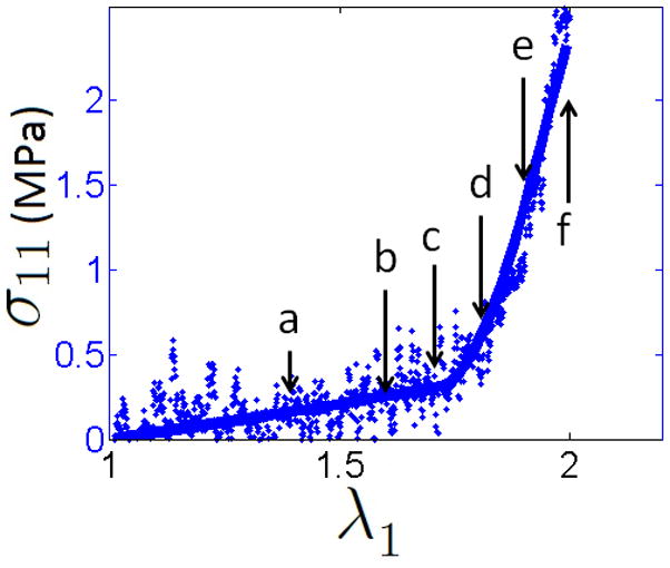
Raw (blue dots) and fitted (blue line) data from uniaxial extension of a rabbit carotid artery, plotted alongside the recruitment function (green line) (associated MPM images given in Fig. 6).

Figure 6.

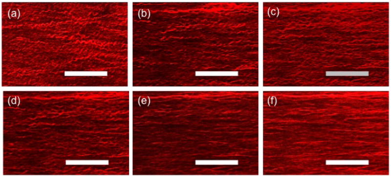
Multi-photon images (MetaMorph) of collagen at stretches of (a) 1.40, (b) 1.60, (c) 1.70, (d) 1.80, (e) 1.90, and (f) 2.00, corresponding to Fig. 6. Bars = 50μm

At the two lowest stretch values, the collagen fibers appear visually to all be crimped while a combination of crimped and uncrimped fibers can be seen at intermediate stretch values, (Fig. 6). The most dramatic recruitment appears in Fig. 6d–e. corresponding to stretches of 1.8 and 1.9. By a stretch of 2.0, the fibers appear to be nearly uniformly uncrimped. These observations were confirmed by the quantitative assessment of tortuosity (Fig. 3 second row, middle column), with recruitment commencing at λ_a1 = 1.7 and tortuosity monotonically decreasing with increasing tissue stretch. This close relationship between initiation of fiber recruitment (λ₁ = 1.7) and departure from the toe region can be seen in Fig. 3 (third row, middle column and Table 2).

Table 2.

Geometric measurements, distribution function parameters, and material constants (± 95% confidence interval) determined by the least-squares fit to the stress-stretch data from uniaxial testing of rabbit carotidarteries, with averages of parameters.

Sample	01	02	03	04	05	06	07	08	AVG
Geometry
C (mm)	4.3	4.2	4.0	4.2	4.0	4.3	4.5	4.2	4.2
L0 (mm)	2.0	2.0	2.0	2.0	2.0	2.0	2.0	2.0	2.0
w (mm)	4.4	3.6	5.0	3.9	3.8	4.3	4.3	3.7	4.1
H (μm)	112	134	124	116	96	154	102	102	118
Model A
λa1	1.70	1.45	1.40	1.50	1.60	1.50	1.80	1.80	1.59
η0(kPa)	120 ±31	96 ± 38	150 ± 27	220 ± 32	220 ± 69	130 ± 26	87 ± 33	110 ± 63	140
η(GPa)	5.5 ± 13	0.13 ± 0.081	0.49 ± 0.26	2.0 ± 1.6	3.1 ± 8.7	5.4 ± 8.6	6.5 ± 9.8	6.2 ± 18	9.8
γ	19 ± 6.7	15 ± 2.9	23 ± 2.9	21 ± 3.2	18 ± 8.6	24 ± 5.8	20 ± 4.3	18 ± 7.6	20
R2	0.9974	0.9990	0.9994	0.9993	0.9965	0.9989	0.9972	0.9940
Model B
λa1	1.70	1.45	1.40	1.50	1.60	1.50	1.80	1.80	1.59
η0(kPa)	140 ± 28	100 ± 35	160 ± 25	230 ± 27	230 ± 66	140 ± 26	140 ± 17	160 ± 52	160
η(MPa)	3.4 ± 1.6	2.6 ± 0.8	1.3 ± 0.4	4.5 ± 1.1	11 ± 5.8	3.1 ± 1.4	0.36 ± 0.16	3.4 ± 2.3	3.7
γ	6.0 ± 2.2	3.8 ± 1.1	6.8 ± 1.0	4.8 ± 1.1	2.7 ± 3.2	6.3 ± 2.4	8.7 ± 0.97	6.4 ± 2.4	5.7
R2	0.9977	0.9990	0.9994	0.995	0.9966	0.9988	0.9990	0.9950
Model C
λa1	1.00	1.00	1.00	1.00	1.00	1.00	1.00	1.00	1.00
α	32 ± 39	16 ± 3.3	130 ± 74	8.3 ± 5.3	62 ± 40	14 ± 36	40 ± 46	24 ± 41	41
β ( × 10−3)	34 ± 45	65 ± 14	6.0 ± 3.4	180 ± 150	14 ± 9.0	110 ± 360	22 ± 26	41 ± 74	59
R2	0.9287	0.9977	0.9944	0.9755	0.9886	0.8718	0.9403	0.8585
η0(kPa)	130 ± 24	83 ± 28	140 ± 40	110 ± 52	230 ± 55	120 ± 24	77 ± 38	75 ± 62	120
η(MPa)	22 ± 2.1	15 ± 1.0	4.2 ± 0.45	54 ± 5.2	12 ± 1.3	120 ± 11	6.3 ± 0.79	17 ± 2.5	31
R2	0.9977	0.9991	0.9978	0.9982	0.9969	0.9988	0.9947	0.9930
Model D
λa1	1.70	1.45	1.40	1.50	1.60	1.50	1.80	1.80	1.59
α	2.5 ± 3.0	2.4 ± 0.22	9.4 ± 5.3	1.1 ± 0.018	3.3 ± 1.3	2.0 ± 3.8	3.5 ± 3.5	1.5 ± 2.3	3.2
β ( × 10−2)	67 ± 120	54 ± 6.5	5.4 ± 3.1	530 ± 23	22 ± 9.2	250 ± 1000	22 ± 24	74 ± 160	130
R2	0.9198	0.9996	0.9942	1.0000	0.9957	0.9012	0.9568	0.8809
η0(kPa)	140 ± 240	110 ± 28	140 ± 47	180 ± 44	260 ± 53	140 ± 23	90 ± 40	110 ± 60	150
η(MPa)	84 ± 8.0	37 ± 2.6	11 ± 1.4	150 ± 14	47 ± 5.5	390 ± 36	20 ± 2.8	46 ± 7.0	98
R2	0.9976	0.9990	0.9972	0.9984	0.9969	0.9987	0.9939	0.9927

C = vessel circumference, L₀ = specimen initial length, w = specimen width, H = thickness.

The initiation of collagen recruitment at finite strain (λ_a1 > 1.0) was seen in all eight samples, (Fig. 7). Further, initiation of recruitment as demonstrated by non-zero values of d_a(λ₁) was always found at stretches close to the end of the toe region. Inter-specimen variability is visible in the magnitudes of d₁ arising from the variation in percentage of fibers recruited. For example, even at the largest values of stretch, less than 6% of the fibers are recruited for Sample 06, whereas Samples 05 and 07 reach nearly 80%.

Figure 7.

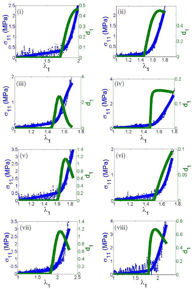
Raw mechanical data from the uniaxial device (blue dots), with fitted response (blue line) and fiber recruitment distribution function d₁ of model D. Specimens 01–08 are labeled with Roman numerals.

4.2. Fiber Orientation

Fiber tracings were made on 3D stacks, making it possible to assess the planarity of the fibers. The 2D superimposed stacks revealed the dispersion of fibers in the e₁ ⊗ e₂ plane (Fig. 8, upper left). This image was rotated by 90° about the e₂ axis to reveal the fiber dispersion along the blood flow direction, in the e₂ ⊗ e₃ plane (Fig. 8, right), and it was rotated by 90° about the e₁ axis to reveal the fiber dispersion in the e₁ ⊗ e₃ plane (Fig. 8, bottom). The angle between the fiber and e₁ was evaluated for a projection of the fiber on the e₁ ⊗ e₂ and e₁ ⊗ e₃ planes. The results for all fiber traces at the activation stretch can be seen in Fig. 9. The average angles for the these two projections were found to be 9.25° ± 2.4° and 1.6° ± 0.74°, respectively, suggesting the fibers can be modeled as planar in distribution.

Figure 8.

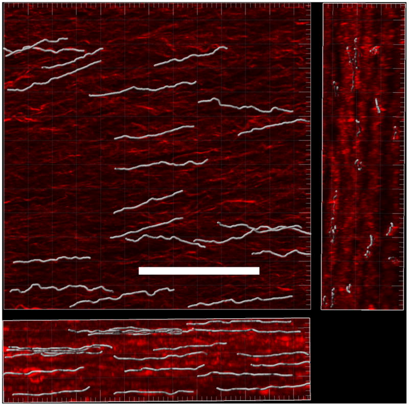
3D reconstruction of multipho-ton image stacks with superposed fiber tracings shown in white. Three orientations are shown with largest image for the e₁ ⊗ e₂, the right image for the e₂ ⊗ e₃ plane, and the bottom image of the e₁ ⊗ e₃ plane, Bar = 50μm.

Figure 9.

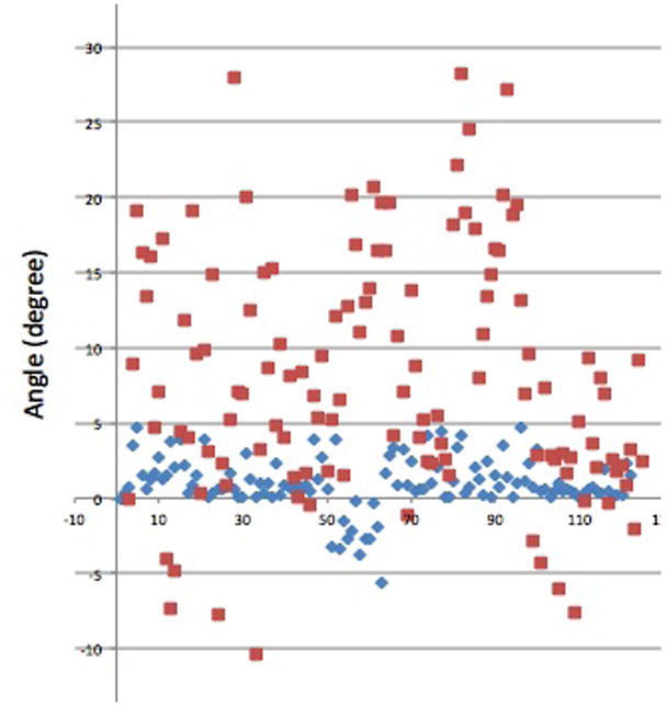
Distribution of magnitude of angle between fiber and e₁ axis for (a) projection on e₁ ⊗ e₂ plane (red) and (b) projection on e₁ ⊗ e₃ plane (blue).

4.3. Constitutive Modeling

Data from each specimen was well fit by all models (Table 2), with R² values close to unity. The directly measured recruitment function enabled a very good fit of the material response, including the transition region, using a simple Neo-Hookean model (Models C and D, Fig. 7). When gradual recruitment was idealized as abrupt (Models A, B), a more complex exponential model for the anisotropic collagen mechanism was used to fit the data. In these cases, even these simple abrupt models worked well.

5. Discussion

Gradual collagen fiber recruitment has been hypothesized to be the underlying mechanism for the highly nonlinear mechanical stiffening seen with increasing stress in arteries (Roach and Burton, 1957). However, the recruitment process has never been directly measured. In this work, we used a custom uniaxial tension device combined with multi-photon microscopy to directly evaluate this process. This approach enabled 3D collagen fiber architecture to be imaged at multiple stretch values for the same sample. Thus, a single specimen could provide multiple data points and comparisons could be made between the level of crimp throughout the loading process. In contrast, when traditional techniques of staining and fixation are used, a single tissue sample can only provide structural information at a single level of stretch. Fiber tortuosity was measured from 3D fiber traces obtained in 3D rendered MPM images. Fiber orientation was measured in projected stacks of images. Collagen recruitment was observed to initiate at a finite strain, corresponding to a sharp steepening of the measured mechanical stiffness, confirming the previous hypothesis. Based on this data, we introduced a new combined constitutive model in which fiber recruitment begins at a finite stretch with activation stretch represented by a probability distribution function. By directly including this recruitment data, the collagen contribution could be modeled using a simple Neo-Hookean model. As a result, only a single phenomenological material constant was needed for the collagen mechanism.

For comparison, three other models for the arterial wall were considered with less structural information. Model A included the least structural data. The fiber orientation was idealized as entirely circumferential, and the nonlinear stiffening behavior after the toe region was modeled with an exponential function beginning at a critical stretch. The only structural parameter was the activation stretch, λ_a1. The abrupt recruitment Model B was similar to Model A, except the measured distribution of collagen orientation data (structural data ρ(θ)) was included rather than idealizing the fibers as purely circumferential. For both models, three parameters were determined from a least squares fit to the stress/stretch data (phenomenological) (η₀, η, and γ). Models A and B can also be used as purely phenomenological models when structural data for λ_a1 by including this constant in the least squares fit. For both Models C and D the orientation distribution and the fiber recruitment distribution were directly measured. The recruitment distribution was fit with a probability distribution function and the distribution of orientation data was used directly. Model D goes beyond Model C by also including the initiation of recruitment at finite strain. Namely, it employs a distribution of collagen recruitment stretches d₁(λ_a) beginning at the directly measured activation stretch, λ_a1.

Despite differences in levels of idealization, the R² value for all models was close to unity in all eight samples (Table 2). The good fit of the data by Models A and B and the ability of this model to capture the initiation of recruitment at finite strain, support the use of Model B in cases when structural information is not available. However, to gain further insights into the mechanism behind the mechanical response of the vessel wall, more structurally-motivated models are necessary. For example, Models A, B and D include a material parameter for the onset of collagen recruitment at finite strain. They are therefore able to model the increase in unloaded radius when elastin is chemically or mechanically eliminated as a load bearing mechanism (e.g. Wulandana and Robertson (2005); Li and Robertson (2009a,b)).

While Model C is capable of fitting the mechanical loading data, it is clear that it does not capture the underlying structural response properly, since collagen recruitment is idealized as initiating at zero strain. The physiological regime for vessels is believed to occur at or above the level where the load curve steepens (see, e.g. Holzapfel et al. (2000)). If so, in the 8 arteries considered here, physiological stretch would be greater than 1.4. Hence, constitutive models with λ_a1 = 1, such as Model C, would require some collagen fibers (those recruited close to the unloaded state) to be laid down during collagen turnover at a stretch greater than 1.4. Burton reported the maximum collagen fiber stretch reached before the yield point to be 1.5 (Burton, 1954). It does not seem plausible that vascular cells would be capable of laying down collagen fibers at this stretch, nor that it would be desirable for collagen fibers to be deposited at stretches near their failure point.

It should be emphasized, that for Models A and B, an exponential function was needed to capture the transition from toe region to the stiff, collagen dominated response. In contrast, Models C and D successfully predicted this transition with a Neo-Hookean model by using a directly measured recruitment function. Consequently, only two fitted material parameters (η₀ and η) were necessary for these more structurally motivated models.

3D measurements of orientation revealed that medial collagen fibers lie predominantly in a single plane, supporting the choice of fan splay for medial collagen orientation in these vessels rather than, for example, conical splay which is commonly used in the literature (e.g. Holzapfel and Ogden (2010); Li and Robertson (2009b)).

There are some limitations to this study. Biaxial inflation/extension is more clinically relevant than the uniaxial loading considering here, though more challenging for structural measurements. With the inclusion of directly measured structural information of collagen orientation this limitation is lessened. The average wall thickness to diameter of the vessels used here was 0.087 mm ± 0.014 mm. Hence, the strain induced during opening the vessel will be insignificant compared with the recruitment stretch. Dogbone shaped specimens were used to diminish some of the end effects from using grip displacement rather than local strain measurements. Further, the fiber recruitment stretch is reported in terms of the tissue stretch along the circumference rather than the angle-dependent fiber stretch. Medial collagen fibers are tightly clustered about the circumferential direction, so this method is deemed acceptable. Furthermore, coupling between the isotropic and anisotropic components, residual stresses, and time-dependent effects (e.g. Bischoff et al. (2004)) are not considered in this work.

In this work, we consider only the medial collagen contribution. In our preliminary studies, adventitial collagen does not appear to be recruited until the largest stretch levels. For example, Fig. 10 shows an image of adventitial collagen under a stretch of 2.0 from sample 07, exhibiting undulations. The process of recruitment of adventitial collagen is the subject of a current study.

Figure 10.

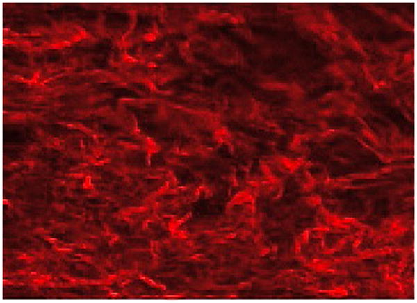
MPM image of adventitial collagen at λ = 2.0 for Sample 07.

While the qualitative response of the specimens is similar, inter-specimen variability in material constants was found, in particular for η. We conjecture the variability in percentage of recruited fibers over the deformation is the source of this variability. For example in samples 03 and 06, the maximum stress is approximately the same, but proportion of recruited fibers is much smaller in sample 06 (15% versus nearly 100%) leading to a much larger value of η for sample 06 (395 MPa compared with 11.34 MPa). Exploration of the cause for this variability is the subject of ongoing work. In the current study, we are not attempting to provide material constants that are generally applicable to all rabbit carotid arteries. Rather, the focus is the demonstration that for each of these arteries, fiber recruitment initiates at a finite strain and can be well modeled using a relatively simple structural model. This is a subject that warrants further study and is a common challenge in vascular mechanics (Sacks, 2000).

Though some technical aspects of the current approach can be refined, this work presents a new theoretical and non-destructive approach for direct inclusion of measured collagen fiber orientation and recruitment in a structurally motivated constitutive model of the artery wall. While other methods such as SALS may be used to non-destructively measure orientation distribution under loading (Sacks, 2003), the method presented here offers the ability to distinguish individual collagen fibers from other tissue structures during loading and provides data at slices throughout the thickness, enabling 3D reconstruction of the fiber structure and 3D fiber tracing.

Collagen recruitment was found to initiate at finite stretch in all samples. These results have important implications for vessels in which the low strain mechanism is damaged, such as during balloon angioplasty. Our work is also important because the methods introduced here provide a means of assessing collagen recruitment during different stages of growth and remodeling. In particular, it has the potential to be used to evaluate collagen deposition stretch.

References

- Arkill KP, Moger J, Winlove CP. The structure and mechanical properties of collecting lymphatic vessels: an investigation using multimodal nonlinear microscopy. J Anat. 2010;216:547–555. doi: 10.1111/j.1469-7580.2010.01215.x. [DOI] [PMC free article] [PubMed] [Google Scholar]
- Barra J, Armentano R, Levenson J, Fischer E, Pichel R, Simon A. Assessment of smooth muscle contribution to descending thoracic aorta elastic mechanics in conscious dogs. Circulation Research. 1993;73:1040–1050. doi: 10.1161/01.res.73.6.1040. [DOI] [PubMed] [Google Scholar]
- Bischoff JE, Arruda EM, Grosh K. A rheological network model for the continuum anisotropic and viscoelastic behavior of soft tissue. Biomechanics and Modeling in Mechanobiology. 2004;3:56–65. doi: 10.1007/s10237-004-0049-4. [DOI] [PubMed] [Google Scholar]
- Burton A. Relation of structure to function of the tissues of the wall of blood vessels. Physiol Rev. 1954;34:619–642. doi: 10.1152/physrev.1954.34.4.619. [DOI] [PubMed] [Google Scholar]
- Chaudhuri B, Kundu P, Sarkar N. Detection and gradation of oriented texture. Patt Recog Lett. 1993;14:147–153. [Google Scholar]
- Courtney T, Sacks M, Stankus J, Guan J, Wagner W. Design and analysis of tissue engineering scaffolds that mimic soft tissue mechanical anisotropy. Biomaterials. 2006;27(19):3631–3638. doi: 10.1016/j.biomaterials.2006.02.024. [DOI] [PubMed] [Google Scholar]
- Dorrington K, McCrum N. Elastin as a rubber. Biopolymers. 1977;16:1201–1222. doi: 10.1002/bip.1977.360160604. [DOI] [PubMed] [Google Scholar]
- Elbischger PJ. PhD Thesis. Graz University of Technology; Graz, Austria: 2005. Computer Vision Methods for the Automatic Analysis of Fibrous Structures in Biological Soft Tissues. [Google Scholar]
- Freed A. Anisotropy in hypoelastic soft-tissue mechanics. i theory. J Mech Mater Struct. 2008;3:911–928. [Google Scholar]
- Freed A, Einstein D, Vesely I. Invariant formulation for dispersed transverse isotropy in aortic heart valves: an efficient means for modeling fiber splay. Biomech Model Mechanobiol. 2005;4:100–117. doi: 10.1007/s10237-005-0069-8. [DOI] [PubMed] [Google Scholar]
- Gasser T, Ogden R, Holzapfel G. Hyperelastic modelling of arterial layers with distributed collagen fibre orientations. J R Soc Interface. 2006;3:15–35. doi: 10.1098/rsif.2005.0073. [DOI] [PMC free article] [PubMed] [Google Scholar]
- Hill MR, Robertson AM. Combined histological and mechanical evaluation of isotropic damage to elastin in cerebral arteries. Proceedings of the 6th World Congress on Biomechanics; Singapore. 2010. [Google Scholar]
- Holzapfel G, Gasser T, Ogden R. A new constitutive framework for arterial wall mechanics and a comparative study of material models. Journal of Elasticity. 2000;61(1–3):1–48. [Google Scholar]
- Holzapfel GA, Ogden RW. Constitutive modelling of arteries. Proceedings of the Royal Society A: Mathematical, Physical and Engineering Sciences. 2010;466(2118):1551–1597. [Google Scholar]
- Humphrey J. Remodeling of a collagenous tissue at fixed lengths. ASME J Biomech Eng. 1999;121:591–597. doi: 10.1115/1.2800858. [DOI] [PubMed] [Google Scholar]
- Humphrey J, Rajagopal K. A constrained mixture model for arterial adaptations to a sustained step change in blood flow. Biomech Model Mechanobiol. 2003;2:109–126. doi: 10.1007/s10237-003-0033-4. [DOI] [PubMed] [Google Scholar]
- Karlon W, Covell J, McCulloch A, Hunter J, Owens J. Automated measurement of myofiber disarray in transgenic mice with ventricular expression of ras. Anat Rec. 1998;252(4):612–625. doi: 10.1002/(SICI)1097-0185(199812)252:4<612::AID-AR12>3.0.CO;2-1. [DOI] [PubMed] [Google Scholar]
- Lanir Y. A structural theory for the homogeneous biaxial stress-strain relationships in flat collagenous tissues. J Biomech. 1979;12:423–436. doi: 10.1016/0021-9290(79)90027-7. [DOI] [PubMed] [Google Scholar]
- Lanir Y. Constitutive equations for fibrous connective tissues. J Biomech. 1983;16:1–12. doi: 10.1016/0021-9290(83)90041-6. [DOI] [PubMed] [Google Scholar]
- Lanir Y. Plausibility of structural constitutive equations for isotropic soft tissues in finite static deformations. J Appl Mech. 1994;61:695–702. [Google Scholar]
- Li D, Robertson A. A structural multi-mechanism constitutive equation for cerebral arterial tissue. Int J Solid Struct. 2009a;46:2920–2928. [Google Scholar]
- Li D, Robertson A. A structural multi-mechanism damage model for cerebral arterial tissue. ASME J Biomech Eng. 2009b;131(10):101013. doi: 10.1115/1.3202559. [DOI] [PubMed] [Google Scholar]
- Megens R, Reitsma S, Schiffers P, Hilgers R, Mey JD, Slaaf D, oude Egbrink M, van Zandvoort M. Two-photon microscopy of vital murine elastic and muscular arteries. J Vasc Res. 2007;44:87–98. doi: 10.1159/000098259. [DOI] [PubMed] [Google Scholar]
- Meijering E, Jacob M, Steiner JCSP, Hirling H, Unser M. Design and validation of a tool for neurite tracing and analysis in fluorescence microscopy images. Cytometry. 2004;58A:167–176. doi: 10.1002/cyto.a.20022. [DOI] [PubMed] [Google Scholar]
- Roach M, Burton A. The reason for the shape of the distensibility curves of arteries. Can J Biochem Physiol. 1957;35:681–690. [PubMed] [Google Scholar]
- Robertson A, Hill M, Li D. In: Structurally motivated damage models for arterial walls-theory and applicationModelling of Physiological Flows, volume 5 of Modeling, Simulation and Applications. Ambrosi D, Quarteroni A, Rozza G, editors. Springer-Verlag; 2011. [Google Scholar]
- Roy S, Boss C, Rezakhaniha R, Stergiopulos N. Experimental characterization of the distribution of collagen fiber recruitment. Journal of Biorheology. 2010;24(2):84–93. [Google Scholar]
- Sacks M. Biaxial mechanical evaluation of planar biological materials. J Elast. 2000;61:199–246. [Google Scholar]
- Sacks M. Incorporation of experimentally-derived fiber orientation into a structural constitutive model for planar collagenous tissues. ASME J Biomech Eng. 2003;125:280–287. doi: 10.1115/1.1544508. [DOI] [PubMed] [Google Scholar]
- Sacks M, Smith D, Hiester E. A small angle light scattering device for planar connective tissue microstructural analysis. Ann Biomed Eng. 1997;25:678–689. doi: 10.1007/BF02684845. [DOI] [PubMed] [Google Scholar]
- Scott S, Ferguson G, Roach M. Comparison of the elastic properties of human intracranial arteries and aneurysms. Can J Physiol Pharma. 1972;50:328–332. doi: 10.1139/y72-049. [DOI] [PubMed] [Google Scholar]
- Taatjes D, Mossman B, editors. Cell Imaging Techniques: Methods and Protocols. Chap 2. Humana Press Inc; Totowa, NJ: 2006. pp. 15–35. [Google Scholar]
- Valentin A, Cardamone L, Baek S, Humphrey J. Complementary vasoactivity and matrix remodelling in arterial adaptations to altered flow and pressure. J R Soc Interface. 2009;6:293–306. doi: 10.1098/rsif.2008.0254. [DOI] [PMC free article] [PubMed] [Google Scholar]
- Wan W, Yanagisawa H, Gleason R. Biomechanical and microstructural properties of common carotid arteries from fibulin-5 null mice. Annals of Biomedical Engineering. 2010;38:3605–3617. doi: 10.1007/s10439-010-0114-3. [DOI] [PMC free article] [PubMed] [Google Scholar]
- Watton P, Ventikos Y, Holzapfel G. Modelling the mechanical response of elastin for arterial tissue. J Biomech. 2009;42:1320–1325. doi: 10.1016/j.jbiomech.2009.03.012. [DOI] [PubMed] [Google Scholar]
- Wiederhielm C. Distensibility characteristics of small blood vessels. Fed Proc. 1965;24:1075–1084. [PubMed] [Google Scholar]
- Wulandana R, Robertson A. First joint BMES/EMBS Conference. Vol. 1. Atlanta, GA: 1999. Use of a multi-mechanism constitutive model for inflation of cerebral arteries; p. 235. [Google Scholar]
- Wulandana R, Robertson A. An inelastic multi-mechanism constitutive equation for cerebral arterial tissue. Biomech Model Mechanobiol. 2005;4(4):235–248. doi: 10.1007/s10237-005-0004-z. [DOI] [PubMed] [Google Scholar]
- Zoumi A, Lu X, Kassab G, Tromberg B. Imaging coronary artery microstructure using second-harmonic and two-photon fluorescence microscopy. Biophys J. 2004;87:2778–2786. doi: 10.1529/biophysj.104.042887. [DOI] [PMC free article] [PubMed] [Google Scholar]
- Zulliger M, Fridez P, Hayashi K, Stergiopulos N. A strain energy function for arteries accounting for wall composition and structure. J Biomech. 2004;37:989–1000. doi: 10.1016/j.jbiomech.2003.11.026. [DOI] [PubMed] [Google Scholar]