An anisotropic constitutive model for immersogeometric fluid–structure interaction analysis of bioprosthetic heart valves

Abstract

This paper considers an anisotropic hyperelastic soft tissue model, originally proposed for native valve tissue and referred to herein as the Lee–Sacks model, in an isogeometric thin shell analysis framework that can be readily combined with immersogeometric fluid–structure interaction (FSI) analysis for high-fidelity simulations of bioprosthetic heart valves (BHVs) interacting with blood flow. We find that the Lee–Sacks model is well-suited to reproduce the anisotropic stress–strain behavior of the cross-linked bovine pericardial tissues that are commonly used in BHVs. An automated procedure for parameter selection leads to an instance of the Lee–Sacks model that matches biaxial stress–strain data from the literature more closely, over a wider range of strains, than other soft tissue models. The relative simplicity of the Lee–Sacks model is attractive for computationally-demanding applications such as FSI analysis and we use the model to demonstrate how the presence and direction of material anisotropy affect the FSI dynamics of BHV leaflets.

1. Introduction

The American Heart Association estimates that valvular heart disease has a prevalence of 2.5% in the US population (Benjamin et al., 2017, Chap. 22). Valvular disease can be fatal, but its mortality has been greatly reduced by the introduction of valvular replacement surgery. The most popular class of replacement valves are bioprosthetic heart valves (BHVs), fabricated from chemically-treated biological tissues (Soares et al., 2016). BHVs provide better hemodynamics than mechanical prostheses, but their tissue leaflets are prone to fatigue, limiting the durability of a typical BHV to 10–15 years (Siddiqui et al., 2009). Soares et al. (2016) and Zakerzadeh et al. (2017) extensively reviewed the state of predictive modeling for these tissues. Such modeling may yield new insights that lengthen the lifespans of future BHVs.

The primary load-bearing component of tissue in BHV leaflets is a network of collagen fibers. These fibers are preferentially arranged, providing greater stiffness along a preferred direction. Further, fibers are embedded in the material at varying levels of tortuosity, causing an increasing fraction of them to be pulled taut at higher strains, producing a highly nonlinear stress–strain curve (Fan and Sacks, 2014). Current high-fidelity models (e.g. Sacks et al., 2015; Zhang and Sacks, 2017) for BHV tissues also account for interactions between fibers, inelastic changes to the material’s local stress-free configuration, and other phenomena. However, in the present work, we are primarily concerned with anisotropy and nonlinearity, and phenomenologically modeling these characteristics in a computationally-efficient way with a limited number of parameters.

A technology that has recently shown great promise for valve simulation is isogeometric analysis (IGA) (Hughes et al., 2005). IGA is a paradigm for computational mechanics that unifies design and analysis of engineered devices by approximating unknown fields (e.g. displacement) using the same spline spaces in which design geometries are specified. In addition to simplifying translation of designs into analysis models, IGA can improve the quality of solutions, due to the mathematical properties of the spline spaces used. Morganti et al. (2015) directly compared IGA and traditional finite element analysis (FEA) of heart valve closure, and found IGA to be overwhelmingly more accurate and efficient in that context, outperforming FEA by several orders of magnitude.

Isogeometric thin shell analysis began with the work of Kiendl et al. (2009), who employed geometrically nonlinear kinematics but assumed a linear strain–stress relation (i.e. St. Venant–Kirchhoff material). This work was later generalized in Kiendl et al. (2015) and Buganza Tepole et al. (2015) to include arbitrary hyperelastic constitutive models. These developments were immediately applied to BHV structural analysis in Kiendl et al. (2015), and, shortly thereafter, in BHV fluid–structure interaction (FSI) analysis (Hsu et al., 2015). Because the space through which blood flows around BHV leaflets is not explicitly part of the BHV’s design, IGA cannot be directly applied to the combined fluid–structure system. To address this, Hsu et al. (2015) immersed the design geometry into an independent discretization of the surrounding fluid space, which we refer to as immersogeometric analysis. Previous immersogeometric BHV simulations have assumed that the distribution of collagen fiber orientations in BHV leaflets is isotropic, but this limits model fidelity. The assumption of isotropy was not due to any fundamental shortcoming of previous frameworks for modeling hyperelastic thin shells; Buganza Tepole et al. (2015) included some simple examples of anisotropic materials. Instead, the absence of material anisotropy from previous isogeometric BHV models largely stemmed from challenges in specifying and calibrating an appropriate anisotropic model.

This work models BHV leaflets with a transversely isotropic constitutive relation originally introduced for mitral valve simulations by Lee et al. (2014). We call it the Lee–Sacks model, after the first and corresponding authors of the cited reference. The model’s strain-energy functional contains a neo-Hookean term and a convex combination of fully-isotropic and transversely-isotropic exponential terms. This permits tuning of the nonlinear stress–strain response by managing the ratio of neo-Hookean and exponential contributions to the strain-energy functional, and also allows for fine tuning of anisotropy within the exponential contributions. In the present work, we demonstrate how this model is formulated within the framework of Kiendl et al. (2015) and obtain the material parameters with an automatic data-fitting algorithm. We find that, with the right parameters, the Lee–Sacks model is able to closely approximate the biaxial stress–strain data collected by Sun and Sacks (2005) from exogenously cross-linked pericardium. This is not a trivial result, as other widely-used soft tissue models are not able to match the same data set as closely (e.g. Kim et al., 2006; Gilmanov et al., 2017).

This paper is organized as follows: Section 2 brifely reviews the hyperelastic Kirchhoff–Love thin shell formulation of Kiendl et al. (2015) and explains how to implement the Lee–Sacks constitutive model within this framework. We verify our implementation by reproducing analytical results and identify parameters for the Lee–Sacks model that best fit the stress–strain data of Sun and Sacks (2005) for BHV leaflets. Section 3 explores the effects of anisotropy on BHV leaflet strain patterns using immersogeometric FSI analysis. Section 4 summarizes our findings and outlines future steps.

2. Formulation and methods

2.1. Shell structural formulation

BHV leaflets are modeled as hyperelastic Kirchhoff–Love thin shells and discretized isogeometrically, as in Kiendl et al. (2015) and Hsu et al. (2015). Precise definitions of the shell geometry and kinematics are given in Appendix A. The weak form of the shell structural formulation is

$${\int }_{{\mathrm{\Gamma }}_0}\mathbf{w}·\rho h_{\text{th}}{\frac{{\partial }^2\mathbf{y}}{\partial t^2}|}_{\mathbf{X}}\mathrm{d}\mathrm{\Gamma }+{\int }_{{\mathrm{\Gamma }}_0}{\int }_{\frac{-h_{\text{th}}}{2}}^{\frac{h_{\text{th}}}{2}}\delta \mathbf{E}:\mathbf{S}\mathrm{d}{\xi }^3\mathrm{d}\mathrm{\Gamma }-{\int }_{{\mathrm{\Gamma }}_0}\mathbf{w}·\rho h_{\text{th}}\mathbf{f}\mathrm{d}\mathrm{\Gamma }-{\int }_{{\mathrm{\Gamma }}_t}\mathbf{w}·{\mathbf{h}}^{\text{net}}\mathrm{d}\mathrm{\Gamma }=0,$$ (1)

where y is the midsurface displacement, the derivative ∂(·)/∂t|_X holds material coordinates X fixed, ρ is the density, S is the second Piola–Kirchhoff stress, ∂E is the variation of the Green–Lagrange strain corresponding to displacement variation w, f is a prescribed body force, h^net is the total traction from the two sides of the shell, and Γ₀ and Γ_t are the shell midsurfaces in the reference and deformed configurations. The Green–Lagrange strain is $\mathbf{E}=\frac{1}{2}(\mathbf{C}-\mathbf{I})$, where C is the right Cauchy–Green deformation tensor and I is the identity tensor. The second Piola–Kirchhoff stress tensor is obtained from a hyperelastic strain-energy density functional ψ: S = ∂_Eψ. In this work, we assume the material to be incompressible; the elastic strain-energy functional ψ_el is augmented by a constraint term enforcing $J=\sqrt{\text{det }\mathbf{C}}=1$, via a Lagrange multiplier p: ψ = ψ_el − p(J − 1).

2.2. Lee–Sacks constitutive model

We model the constitutive behavior of BHV leaflets using a transversely isotropic model introduced in Lee et al. (2014), which we term the Lee–Sacks model. This model’s strain-energy functional uses a neo-Hookean term to model the extracellular matrix and a convex combination of fully-isotropic and transversely-isotropic exponential-type terms to model the network of collagen fibers. The model is given by

$${\psi }_{\mathit{\text{el}}}(I_1,I_4)=\frac{c_0}{2}(I_1-3)+\frac{c_1}{2}(\delta e^{c_2{(I_1-3)}^2}+(1-\delta )e^{c_3{(I_4-1)}^2}-1),$$ (2)

where c₀, c₁, c₂, c₃ are material parameters and δ ∈ [0, 1] is a parameter that determines the level of anisotropy. I₁ = tr C and I₄ = m · C m, where m is a unit vector defining the collagen fiber direction in the reference configuration. Based on the structure of the bovine pericardium used in BHVs, we assume that collagen fibers lie primarily in the plane of the tissue (i.e., m³ = 0 in the curvilinear coordinate system of Appendix A).

Note that the exponential anisotropic term asymptotically dominates the isotropic term with increasing strain; exponential functions grow faster than polynomials. Therefore, for any ε > 0, no matter how small, if δ = 1 − ε, there exists a strain level beyond which the anisotropic term dominates. In view of this, δ should be interpreted as a measure of when anisotropy dominates, rather than whether.

2.3. Implementation verification

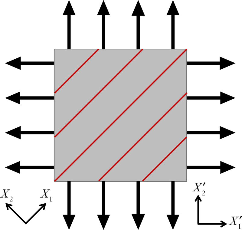
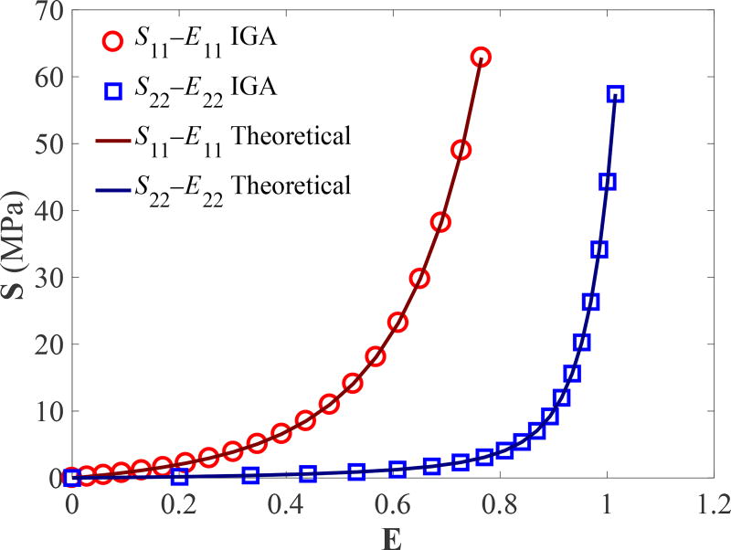
To verify the Lee–Sacks model implementation, we perform IGA simulations of biaxial tensile tests and compare the results with theoretical solutions. We adopt the static, stress-controlled equibiaxial testing setup of Sacks and Sun (2003), in which the magnitude of nominal stress imposed on each side of the specimen is identical (Figure 1). The Cartesian material coordinates X₁ and X₂ are oriented at a 45° angle relative to the Cartesian specimen coordinates $X_1^{\prime }$ and $X_2^{\prime }$. The fiber direction m is aligned with X₁. We simulate the equibiaxial tests using one cubic B-spline element. The material parameters from Lee et al. (2014) (with some changes in notation) are used: c₀ = 0.2 MPa, c₁ = 2.8351 MPa, c₂ = 0.4252, c₃ = 0.4316, and δ = 0.4231. The nominal stress imposed on each side of the specimen varies from 0 MPa to 100 MPa. Following Sun and Sacks (2005), computed strains from the IGA simulations are used (in Eq. (A.3)) to calculate the theoretical stresses. Figure 2 shows the components of E and S reported based on X₁ and X₂; the stress–strain relationships are in perfect agreement between IGA and theoretical solutions.

Figure 1.

Stress-controlled equibiaxial testing setup from Sun and Sacks (2005). Black arrows on edges represent nominal stresses, which are identical in magnitude on each side of the specimen. Red lines represent fiber orientation.

Figure 2.

Verification of the Lee–Sacks model implementation using the equibiaxial tests.

Remark 1

While the stress values considered here exceed those used in comparable experiments, the goal of this section is not to compare with experimental data, but to verify that the numerical method correctly approximates the Lee–Sacks constitutive model, which imposes no limits on stress levels. The stress range selected more clearly illustrates the exponential behavior of the stress–strain relation than smaller ranges.

2.4. Parameterization of the Lee–Sacks material model

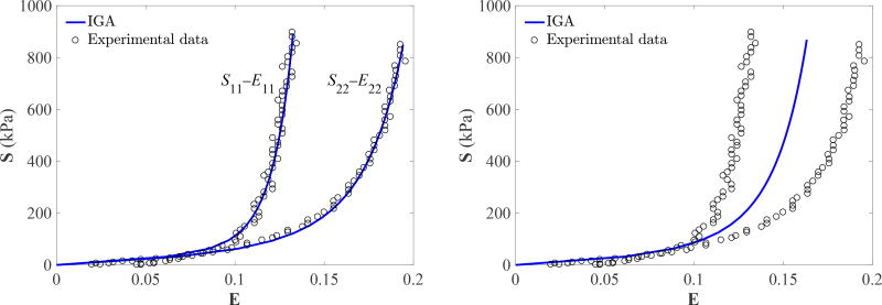
The material parameters of the Lee–Sacks model for BHV simulations are determined based on a set of biaxial mechanical experimental data reported by Sun and Sacks (2005), in which the stress–strain relationship of a 25 mm × 25 mm square glutaraldehyde-treated bovine pericardium (GLBP) specimen is probed by performing stress-controlled equibiaxial tests as shown in Figure 1. The stress–strain experimental data sets of S₁₁–E₁₁ and S₂₂–E₂₂, shown in Figure 3, are reported based on the material axes X₁ and X₂. The experimental data for 11 and 22 components of stress and strain are not collated into pairs of the form ((S₁₁, S₂₂), (E₁₁, E₂₂)), so tensor-valued experimental strains are not available to plug into the function S(E) given by the material model. We simulate the equibiaxial tests using IGA with one cubic B-spline element. The nominal stress imposed on each side of the specimen varies from 0 to 1 MPa, and 20 simulations are performed within this range. The stress–strain data points generated using IGA simulations are interpolated using cubic B-spline curves for comparison with experimental data points.

Figure 3.

Fitting results for experimental data reported in Sun and Sacks (2005) using the Lee–Sacks material model. Left: The anisotropic case. Right: The isotropic case.

The material parameters, c₀, c₁, c₂, c₃, and δ, in Eq. (2) are determined by fitting the predicted stress–strain curves to the corresponding experimental data set. For the fitting process, we used the function fminsearch in the Optimization Toolbox of MATLAB, with the Nelder–Mead simplex direct search algorithm (Nelder and Mead, 1965; Lagarias et al., 1998) and the default termination criterion, to maximize the coefficient of determination, R², defined by

$$R^2=1-\frac{{\sum }_{i=1}^N{(S_i^{\text{exp}}-S_i^{\text{IGA}})}^2}{{\sum }_{i=1}^N{(S_i^{\text{exp}}-{\overline{S}}^{\text{exp}})}^2},$$ (3)

where $S_i^{\text{exp}}$ and $S_i^{\text{IGA}}$ are the S_aa in the experimental data set and from the IGA simulations, respectively, S̄^exp is the mean of S_aa in the experimental data set, and N is the number of data points.

There are two stages in the fitting process: fitting based on the low strain data and fitting based on the complete data. The neo-Hookean component in Eq. (2) is mainly responsible for low strain response, so c₀, the shear modulus, is determined first by experimental data in low Green–Lagrange strain (E_aa < 0.08) region. The low-strain cutoff is selected by visually estimating the region of stress–strain data in which points from the 11 and 22 curves in Figure 3 are clustered around a single line passing through the origin. While determining c₀, c₁ is set to zero so only the neo-Hookean term is active. After c₀ is determined, the rest of material parameters, c₁, c₂, c₃, and δ, are determined using the complete experimental data, while holding c₀ fixed.

Because the simplex algorithm only finds a local minimum, we apply it several times using different initial conditions, to examine the sensitivity and select the best result. For the initial optimization of c₀ using low-strain data, ten independent optimization procedures are performed with initial values chosen uniformly from 1 kPa to 10³ kPa. For all initial values, the optimized value for c₀ is 67.6080 kPa. In the second optimization for the remaining parameters, ten starting points are generated via Latin hypercube sampling, performed within the hyper-rectangle 0 ≤ c₁ ≤ 10³ kPa, 0 ≤ c₂ ≤ 100, 0 ≤ c₃ ≤ 100, and 0 ≤ δ ≤ 1. Unlike the optimization for c₀, there is slight (< 1%) variability in the resulting parameters, and the case with the best R² value is selected. The material model in Eq. (2) can also represent isotropic materials; in that case, the second step of the optimization is modified by restricting to δ = 1, which eliminates c₃ entirely. The ranges of the initial values chosen above are based on the numerical experience of the material model used in Hsu et al. (2015).

The parameters resulting from this fitting procedure are listed in Table 1. The corresponding stress–strain curves are shown in Figure 3. For the anisotropic case, the value of R² is 0.9758. These curves match the experimental data more closely, over a wider range of strains, than other soft tissue models found in the literature, e.g., the Fung-type model of Kim et al. (2006, Figure 3) and the May-Newmann–Yin model of Gilmanov et al. (2017, Figure 5).

Table 1.

Parameters of the Lee–Sacks material model (Eq. (2)) for anisotropic and isotropic cases determined by fitting equibiaxial experimental data reported in Sun and Sacks (2005). Note that for the isotropic case, c₃ does not play a role since δ is determined to be 1.

	c0 (kPa)	c1 (kPa)	c2	c3	δ
Anisotropic	67.6080	8.8559	42.4229	72.9215	0.9983
Isotropic	67.6080	13.2848	38.1878	–	1.0000

Figure 5.

(a) The Bézier elements defining the T-spline surface used in the shell analysis. Circumferential and radial directions of the leaflets are represented by “cir” and “rad”, respectively. z is a unit vector that is perpendicular to both circumferential and radial directions. (b) Fiber orientation of 0°. a₃ is the surface normal vector and m is the normalized cross product of z and a₃. (c) Fiber orientation of 45°. (d) Fiber orientation of 90°.

3. Application to FSI analysis of BHVs

3.1. FSI modeling framework and methods

For the simulation of BHV with anisotropic leaflets, the immersogeometric FSI techniques developed in Kamensky et al. (2015b,a) and Hsu et al. (2014, 2015) are utilized. The computational setup used in this work is shown in Figure 4, while the details are given in Appendix B. The blood flow in the deforming artery is governed by the Navier–Stokes equations of incompressible flow posed on a moving domain. The domain motion is handled using the Arbitrary Lagrangian–Eulerian (ALE) formulation (Donea et al., 1982) and follows the motion of the deformable arterial wall, which is governed by equations of large-deformation elastodynamics written in the Lagrangian frame (Bazilevs et al., 2008). The ALE Navier–Stokes subproblem is discretized using the variational multiscale approach (Bazilevs et al., 2007).

Figure 4.

A view of the arterial wall and lumen into which the valve is immersed. The suture ring of the BHV intersects with the arterial wall. The left ventricular pressure waveform is obtained from Yap et al. (2011) and has a duration of 0.86 s.

BHV leaflets are modeled as rotation-free hyperelastic Kirchhoff–Love shells presented in Section 2. The BHV is immersed into the moving blood-flow domain; the immersed FSI problem is formulated using an augmented Lagrangian approach and solved using a semi-implicit time integration procedure (Kamensky et al., 2015b,a). Contact between leaflets is handled by a penalty-based approach and imposed at quadrature points of the shell structure (Kamensky et al., 2015b). A combination of the quasi-direct and block-iterative FSI coupling strategies (Tezduyar et al., 2006) is adopted for solving the coupled FSI problem (Hsu et al., 2014).

The arterial wall is modeled as a neo-Hookean material with dilatational penalty (Bazilevs et al., 2008), where the shear and bulk moduli of the model are selected to produce a Young’s modulus of 1.0 × 10⁷ dyn/cm² and Poisson’s ratio of 0.45 in the small-strain limit. The density of the arterial wall is set to 1.0 g/cm³. Mass-proportional damping is added to model the interaction of the artery with surrounding tissue and interstitial fluid, with the damping coefficient set to 1.0 × 10⁴ s⁻¹. The density and dynamic viscosity of blood flow are set to 1.0 g/cm³ and 3.0 × 10⁻² g/(cm s), respectively. The BHV leaflet density and thickness are set to 1.0 g/cm³ and 0.0386 cm, respectively. The choice of these values is based on the discussions in Hsu et al. (2015) and references therein.

To study the effect of anisotropy due to the fiber orientation, we perform FSI simulations of four cases: one case of isotropic leaflets and three cases of anisotropic leaflets with fiber orientations of 0°, 45°, and 90° as shown in Figure 5. Fiber orientation of 0° is defined by $\mathbf{m}=\frac{\mathbf{z}\times {\mathbf{a}}_3}{\Vert \mathbf{z}\times {\mathbf{a}}_3\Vert }$, where z is a unit vector that is perpendicular to both circumferential and radial directions of the leaflets, as shown in Figure 5a, and a₃ is the normal vector of shell midsurface defined in Appendix A. Vectors, m, z, and a₃, are illustrated in Figure 5b. With 0° defined, fiber orientations of 45° and 90° are obtained by rotating m about a₃. Fiber orientation of 0° approximates the fiber alignment along the circumferential direction of native aortic valve leaflets (Huang et al., 2007). Fiber orientation of 45° approximates the fiber alignment of typical pericardial BHVs (Sun et al., 2005). Simulations are performed using material parameters listed in Table 1 obtained for the Lee–Sacks constitutive model. The time step size for the FSI simulation is Δt = 1.0 × 10⁻⁴ s.

3.2. Simulation results

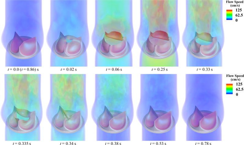
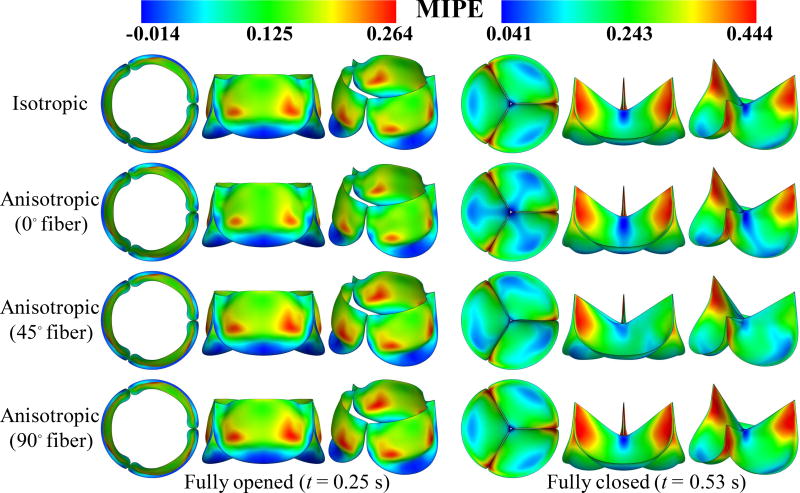
The simulated BHV opens and closes at roughly the same times with all four fiber architectures; we define the fully-opened stage at t = 0.25 s and the fully-closed stage at t = 0.53 s. Figure 6 depicts the flow fields in the artery lumen from a period of the FSI simulation for the case of 45° fiber orientation. The valve opens with the rising left ventricular pressure at the beginning stage of systole (0.0–0.06 s) and stays fully open near the peak systole (0.25 s), allowing sufficient blood flow to enter the ascending aorta. A very quick valve closure, which minimizes the reverse flow into the left ventricle, is observed at the beginning of diastole (0.34–0.38 s). Finally, the valve properly seals and the flow reaches a near-hydrostatic state (0.53–0.78 s).

Figure 6.

Volume rendering of the velocity field at several points during a cardiac cycle for the 45° fiber orientation case. The time t is synchronized with the pressure profile in Figure 4.

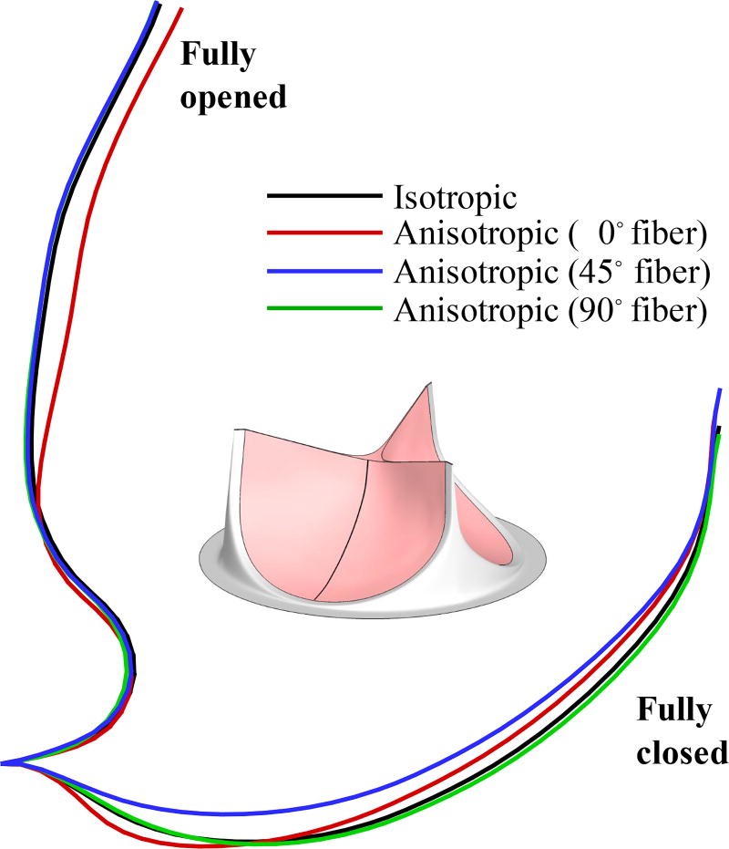
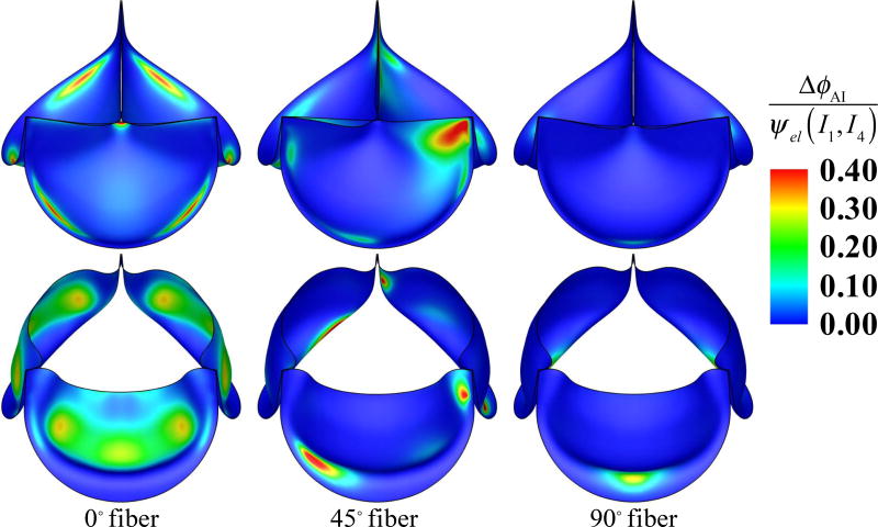
Figure 7 illustrates the deformations and strain distributions of the BHV and Figure 8 shows the displacement of cross-sections of the leaflet in the fully-closed and full-opened stages, for different fiber architectures. Figure 9 illustrates the ratio of I₄ contribution to the strain-energy density functional ψ_el for the anisotropic cases, viz.

$$\frac{\mathrm{\Delta }{\varphi }_{\text{AI}}}{{\psi }_{\mathit{\text{el}}}(I_1,I_4)},$$ (4)

where

$$\mathrm{\Delta }{\varphi }_{\text{AI}}=\frac{c_1}{2}(1-\delta )(e^{c_3{(I_4-1)}^2}-e^0).$$ (5)

Figure 7.

Deformations of the valve from the FSI simulations, colored by the maximum in-plane principal Green–Lagrange strain (MIPE) evaluated on the aortic side of the leaflet. Note the different color scales used for fully-opened and fully-closed results.

Figure 8.

Cross-sectional profiles of the fully-opened and fully-closed leaflets.

Figure 9.

The ratio of I₄ contribution to the strain-energy density functional for different fiber orientation cases at fully-closed (top) and fully-opened (bottom) stages.

3.3. Discussion

Figures 7 and 8 show that, at the fully-opened stage, the 0° case has strains slightly lower than other cases. However, its valve opening size (geometric orifice area) is noticeably smaller than all other cases. This effect is explained by Figure 9: the anisotropic contribution Δϕ_AI for the 0° case is pronounced on almost the entire leaflet at the fully-opened stage, whereas the contribution of Δϕ_AI is relatively small in both 45° and 90° cases.

Based on the results shown in Figures 7–9, the overall behavior of the 90° fiber orientation case is very close to that of the isotropic case. This is expected, given that leaflets are only tethered at one end along the radial direction, and thus fibers oriented radially are unable to support significant tension. Leaflets are constrained at both ends in the circumferential direction, and we see an accordingly greater proportion of strain energy stored by fibers oriented circumferentially, in the 0° and 45° cases, as illustrated in Figure 9. This is most noticeable in the 45° case, where fibers near one commissure point of each leaflet are nearly parallel to the direction of tension during diastole. This affects the kinematics of the leaflets during closure, by reducing strain at that commissure point, as seen in Figure 7, and minimizing the belly region’s distension during diastole, as seen in Figure 8.

The fact that this asymmetrical configuration utilizes the fibers’ load-bearing capabilities most effectively is perhaps surprising, as one might hypothesize that the symmetrical 0° orientation is more similar to the fiber architecture of a native valve, and therefore optimal. However, fibers in native valves converge toward the commissure points, which is a configuration that cannot be reproduced by cutting tissue samples out from sheets of bovine pericardium. Pericardial leaflets will typically have a global preferred fiber direction, as approximated by the parameterization of the present study, allowing reinforcement of at most one commissure point per leaflet. This is in agreement with the earlier experimental and computational work of Sun et al. (2005) on pericardial BHVs.

4. Conclusions, limitations, and future work

This work combines the isogeometric hyperelastic Kirchhoff–Love thin shell framework with the Lee–Sacks constitutive model and immersogeometric FSI methodology to perform high-fidelity BHV FSI simulations with studies of different fiber orientations and effects of anisotropy. An important finding is that the Lee–Sacks model, while originally proposed for simulating native mitral valve tissue, is also well-suited for reproducing the anisotropic stress–strain behavior of cross-linked bovine pericardium. With an appropriate parameter set, it matches the data of Sun and Sacks (2005) more closely, over a wider range of strains, than other soft tissue models found in the literature. The relative simplicity of the Lee–Sacks model makes it an attractive alternative to more complex high-fidelity structural models (e.g. Fan and Sacks, 2014; Sacks et al., 2015; Zhang and Sacks, 2017) in computationally-demanding applications such as FSI analysis. Our simulation results demonstrate how the presence and direction of anisotropy affect the FSI dynamics of BHV leaflets.

The parameterization of preferred collagen fiber orientation in Section 3.1 suggests a straightforward way to incorporate material anisotropy into parametric design frameworks for prosthetic heart valves (e.g. Xu et al., 2018). This will allow systematic exploration of the combined effects of anisotropy and other geometrical parameters on quantities of interest such as coaptation area and effective orifice area. If joined to a derivative-free optimization algorithm as in Wu et al. (2017), such a framework even opens the door for automatic determination of the best choice of fiber orientation in BHVs using FSI analysis.

While appealing from a computational perspective, the simplicity of the Lee–Sacks model leads to several limitations that we might address in future work. First, the assumption of hyper-elasticity rules out inelastic behavior, such as permanent set, which is critical to understanding long-term changes in BHV mechanics after implantation. Second, the assumption of a single fiber family, oriented along one direction, only approximates the angular distribution of collagen fibers in planar soft tissues. These limitations of the Lee–Sacks model could be addressed without sacrificing computational efficiency in FSI simulations by coupling the FSI analysis with offline solid mechanics computations using higher-fidelity models, such as those discussed by Sacks et al. (2015) and Zhang and Sacks (2017). Another limitation of the FSI computations from this work is that they do not account for variability in aortic geometry; this limitation could be addressed by a more comprehensive study considering material anisotropy within the patient-specific FSI analysis framework of Xu et al. (2018).

Appendix A

Kirchhoff–Love shell theory

The Kirchhoff–Love hypothesis of normal cross sections implies that a point x in the shell continuum can be described by a point r on the midsurface and a vector a₃ normal to the midsurface:

$$\mathbf{x}({\xi }^1,{\xi }^2,{\xi }^3)=\mathbf{r}({\xi }^1,{\xi }^2)+{\xi }^3{\mathbf{a}}_3({\xi }^1,{\xi }^2),$$ (A.1)

where ξ¹, ξ² are midsurface coordinates, ξ³ ∈ [−h_th/2, h_th/2] is the thickness coordinate, and h_th is the shell thickness.

Covariant basis vectors and metric coefficients are defined by g_i = x_,i and g_ij = g_i · g_j, respectively, where (·)_,i = ∂(·)/∂ξⁱ. We adopt the convention that Latin indices take on values {1, 2, 3} while Greek indices take on values {1, 2}. Contravariant basis vectors gⁱ are defined by ${\mathbf{g}}^i·{\mathbf{g}}_j={\delta }_j^i$. Contravariant metric coefficients are given by [g^ij] = [g_ij]⁻¹. The Kirchhoff–Love shell model assumes that

$$g_{\alpha \beta }=a_{\alpha \beta }-2{\xi }^3{b}_{\alpha \beta },$$ (A.2)

where a_αβ = a_α · a_β, b_αβ = a_α,β · a₃, a_α = r_,α, and ${\mathbf{a}}_3=\frac{{\mathbf{a}}_1\times {\mathbf{a}}_2}{\Vert {\mathbf{a}}_1\times {\mathbf{a}}_2\Vert }$. These definitions hold for both deformed and undeformed configurations. Variables of the latter are indicated by (·̊), e.g., x̊, g̊_,i, g̊_ij, etc. Note that the b_αβ term accounts for strains due to bending. The Jacobian determinant of the structure’s motion is $J=\sqrt{|g_{\mathit{\text{ij}}}|/|{\mathring{g}}_{\mathit{\text{ij}}}|}$ and the in-plane Jacobian determinant is $J_o=\sqrt{|g_{\alpha \beta }|/|{\mathring{g}}_{\alpha \beta }|}$.

For incompressible materials, one can use these relations to express E₃₃ in terms of E_αβ (Kiendl et al., 2015, Eq. (38)), formally eliminate the Lagrange multiplier p using the plane-stress condition, S³³ = 0 (Kiendl et al., 2015, Eq. (46)), and derive an in-plane material tangent tensor ℂ̂ such that dS^αβ = ℂ̂^αβγδ dE_γδ, where dS and dE are total differentials of S and E:

$$S^{\alpha \beta }=2\frac{\partial {\psi }_{\mathit{\text{el}}}}{\partial C_{\alpha \beta }}-2\frac{\partial {\psi }_{\mathit{\text{el}}}}{\partial C_{33}}{J}_o^{-2}{g}^{\alpha \beta },$$ (A.3)

$${\widehat{ℂ}}^{\alpha \beta \gamma \delta }=4\frac{{\partial }^2{\psi }_{\mathit{\text{el}}}}{\partial C_{\alpha \beta }\partial C_{\gamma \delta }}+4\frac{{\partial }^2{\psi }_{\mathit{\text{el}}}}{\partial C_{33}^2}{J}_o^{-4}{g}^{\alpha \beta }{g}^{\gamma \delta }-4\frac{{\partial }^2{\psi }_{\mathit{\text{el}}}}{\partial C_{33}\partial C_{\alpha \beta }}{J}_o^{-2}{g}^{\gamma \delta }-4\frac{{\partial }^2{\psi }_{\mathit{\text{el}}}}{\partial C_{33}\partial C_{\gamma \delta }}{J}_o^{-2}{g}^{\alpha \beta }+2\frac{\partial {\psi }_{\mathit{\text{el}}}}{\partial C_{33}}{J}_o^{-2}(2g^{\alpha \beta }{g}^{\gamma \delta }+g^{\alpha \gamma }{g}^{\beta \delta }+g^{\alpha \delta }{g}^{\beta \gamma }).$$ (A.4)

With Eqs. (A.3) and (A.4), arbitrary 3D constitutive models providing $\frac{\partial {\psi }_{\mathit{\text{el}}}}{\partial C_{\mathit{\text{ij}}}}$ and $\frac{{\partial }^2{\psi }_{\mathit{\text{el}}}}{\partial C_{\mathit{\text{ij}}}\partial C_{\mathit{\text{kl}}}}$ can be directly used for shell analysis.

For the Lee–Sacks model of Eq. (2), I₁ and I₄ are given by

$$I_1=\text{tr }\mathbf{C}=g_{\alpha \beta }{\stackrel{\circ }{g}}^{\alpha \beta }+C_{33},$$ (A.5)

$$I_4=\mathbf{m}·\mathbf{\text{ C m}}=m^i{m}^j{g}_{\mathit{\text{ij}}},$$ (A.6)

where m = mⁱ g̊_i is a unit vector defining the collagen fiber direction in the reference configuration at a material point x̊, written in local covariant basis g̊_i. For the choice of ϕ_el in the Lee–Sacks model, the strain energy derivatives required in Eqs. (A.3) and (A.4) are

$$\frac{\partial {\psi }_{\mathit{\text{el}}}}{\partial C_{\mathit{\text{ij}}}}=\frac{1}{2}(c_0+2\delta c_1{c}_2(I_1-3)e^{c_2{(I_1-3)}^2}){\stackrel{\circ }{g}}^{\mathit{\text{ij}}}+(1-\delta )c_1{c}_3(I_4-1)e^{c_3{(I_4-1)}^2}{m}^i{m}^j,$$ (A.7)

$$\frac{{\partial }^2{\psi }_{\mathit{\text{el}}}}{\partial C_{\mathit{\text{ij}}}\partial C_{\mathit{\text{kl}}}}=\delta (1+2c_2{(I_1-3)}^2)c_1{c}_2{e}^{c_2{(I_1-3)}^2}{\stackrel{\circ }{g}}^{\mathit{\text{ij}}}{\stackrel{\circ }{g}}^{\mathit{\text{kl}}}+(1-\delta )(1+2c_3{(I_4-1)}^2)c_1{c}_3{e}^{c_3{(I_4-1)}^2}{m}^i{m}^j{m}^k{m}^l,$$ (A.8)

where we have used

$$\frac{\partial {\psi }_{\mathit{\text{el}}}(I_1,I_4)}{\partial C_{\mathit{\text{ij}}}}=\frac{\partial {\psi }_{\mathit{\text{el}}}}{\partial I_1}\frac{\partial I_1}{\partial C_{\mathit{\text{ij}}}}+\frac{\partial {\psi }_{\mathit{\text{el}}}}{\partial I_4}\frac{\partial I_4}{\partial C_{\mathit{\text{ij}}}},$$ (A.9)

$$\frac{{\partial }^2{\psi }_{\mathit{\text{el}}}(I_1,I_4)}{\partial C_{\mathit{\text{ij}}}\partial C_{\mathit{\text{kl}}}}=\frac{{\partial }^2{\psi }_{\mathit{\text{el}}}}{\partial I_1\partial I_1}\frac{\partial I_1}{\partial C_{\mathit{\text{ij}}}}\frac{\partial I_1}{\partial C_{\mathit{\text{kl}}}}+\frac{{\partial }^2{\psi }_{\mathit{\text{el}}}}{\partial I_4\partial I_4}\frac{\partial I_4}{\partial C_{\mathit{\text{ij}}}}\frac{\partial I_4}{\partial C_{\mathit{\text{kl}}}}+\frac{{\partial }^2{\psi }_{\mathit{\text{el}}}}{\partial I_1\partial I_4}(\frac{\partial I_1}{\partial C_{\mathit{\text{ij}}}}\frac{\partial I_4}{\partial C_{\mathit{\text{kl}}}}+\frac{\partial I_4}{\partial C_{\mathit{\text{ij}}}}\frac{\partial I_1}{\partial C_{\mathit{\text{kl}}}}),$$ (A.10)

$$\frac{\partial {\psi }_{\mathit{\text{el}}}}{\partial I_1}=\frac{1}{2}(c_0+2\delta c_1{c}_2(I_1-3)e^{c_2{(I_1-3)}^2}),$$ (A.11)

$$\frac{\partial {\psi }_{\mathit{\text{el}}}}{\partial I_4}=(1-\delta )c_1{c}_3(I_4-1)e^{c_3{(I_4-1)}^2},$$ (A.12)

$$\frac{{\partial }^2{\psi }_{\mathit{\text{el}}}}{\partial I_1\partial I_1}=\delta (1+2c_2{(I_1-3)}^2)c_1{c}_2{e}^{c_2{(I_1-3)}^2},$$ (A.13)

$$\frac{{\partial }^2{\psi }_{\mathit{\text{el}}}}{\partial I_4\partial I_4}=(1-\delta )(1+2c_3{(I_4-1)}^2)c_1{c}_3{e}^{c_3{(I_4-1)}^2},$$ (A.14)

$$\frac{{\partial }^2{\psi }_{\mathit{\text{el}}}}{\partial I_1\partial I_4}=0,$$ (A.15)

$$\frac{\partial I_1}{\partial C_{\mathit{\text{ij}}}}={\stackrel{\circ }{g}}^{\mathit{\text{ij}}},$$ (A.16)

$$\frac{\partial I_4}{\partial C_{\mathit{\text{ij}}}}=m^i{m}^j.$$ (A.17)

The identities $\frac{{\partial }^2{I}_1}{\partial C_{\mathit{\text{ij}}}\partial C_{\mathit{\text{kl}}}}=\frac{{\partial }^2{I}_4}{\partial C_{\mathit{\text{ij}}}\partial C_{\mathit{\text{kl}}}}=0$ were used to simplify (A.10).

Appendix B

FSI computational setup

We consider an aortic configuration and model the artery as a 16 cm long elastic cylindrical tube with a three-lobed dilation near the BHV region modeling the aortic sinus (Figure 4). The cylindrical portion of the artery has an inside diameter of 2.6 cm and a wall thickness of 0.15 cm. The discretizations of the blood flow domain and the solid arterial wall make use of trivariate quadratic NURBS and are assumed to be conforming at the fluid–solid interface. The BHV leaflet geometry is modeled based on a 23-mm design in Sun et al. (2005) and parametrically generated using the method proposed in Hsu et al. (2015). The leaflets are discretized by T-splines using Bézier elements (Scott et al., 2011). The mesh resolutions are shown in Figures 4 and 5a and are identical to those reported in Hsu et al. (2015). The resolution is similar to that used in the computations of Xu et al. (2018). Appendix A of the cited study documents a systematic convergence testing, and shows the effects of spatial and temporal refinement on clinically-important quantities of interest relating to leaflet kinematics, namely coaptation area and effective orifice area. The results of this testing indicate that those quantities of interest are resolved to within a few percent at the resolution used.

The inflow and outflow boundaries are located at the ventricular and aortic ends of the channel shown in Figure 4. The designations of inflow and outflow are based on the prevailing flow direction during systole. We apply a physiologically-realistic left ventricular pressure waveform (Figure 4) as a traction boundary condition at the inflow. The applied pressure signal is periodic with a period of 0.86 s. The traction −(p₀ + RQ)n is applied at the outflow for the resistance boundary condition (Vignon-Clementel et al., 2006), where p₀ is a constant physiological pressure level, n is the outward-facing normal of the fluid domain, R > 0 is a resistance coefficient, and Q is the volumetric flow rate through the outflow. In the present computation, we set p₀ = 80 mmHg and R = 70 (dyn s)/cm⁵. These values ensure a realistic transvalvular pressure difference of 80 mmHg across a closed valve while permitting a reasonable flow rate during systole.

The inlet and outlet cross sections are free to slide in their tangential planes and deform radially, but constrained not to move in the orthogonal directions (Bazilevs et al., 2010). The outer wall of the artery has a zero-traction boundary condition. The metal frame and suture ring of the BHV are assumed to be rigid and fixed in space; homogeneous Dirichlet conditions are applied to any control point of the solid portion of the artery mesh whose corresponding basis function’s support intersects the stationary metal frame and suture ring. The edges of the BHV leaflets are clamped to the rigid frame.

References

- Bazilevs Y, Calo VM, Cottrel JA, Hughes TJR, Reali A, Scovazzi G. Variational multiscale residual-based turbulence modeling for large eddy simulation of incompressible flows. Computer Methods in Applied Mechanics and Engineering. 2007;197:173–201. [Google Scholar]
- Bazilevs Y, Calo VM, Hughes TJR, Zhang Y. Isogeometric fluid–structure interaction: theory, algorithms, and computations. Computational Mechanics. 2008;43:3–37. [Google Scholar]
- Bazilevs Y, Hsu MC, Zhang Y, Wang W, Kvamsdal T, Hentschel S, Isaksen J. Computational fluid–structure interaction: Methods and application to cerebral aneurysms. Biomechanics and Modeling in Mechanobiology. 2010;9:481–498. doi: 10.1007/s10237-010-0189-7. [DOI] [PubMed] [Google Scholar]
- Benjamin EJ, Blaha MJ, Chiuve SE, Cushman M, Das SR, Deo R, de Ferranti SD, Floyd J, Fornage M, Gillespie C, et al. Heart disease and stroke statistics–2017 update: a report from the American Heart Association. Circulation. 2017;135:e146–e603. doi: 10.1161/CIR.0000000000000485. [DOI] [PMC free article] [PubMed] [Google Scholar]
- Buganza Tepole A, Kabaria H, Bletzinger KU, Kuhl E. Isogeometric kirchhoff–love shell formulations for biological membranes. Computer Methods in Applied Mechanics and Engineering. 2015;293:328–347. doi: 10.1016/j.cma.2015.05.006. [DOI] [PMC free article] [PubMed] [Google Scholar]
- Donea J, Giuliani S, Halleux JP. An arbitrary Lagrangian-Eulerian finite element method for transient dynamics fluid–structure interactions. Computer Methods in Applied Mechanics and Engineering. 1982;33:689–723. [Google Scholar]
- Fan R, Sacks MS. Simulation of planar soft tissues using a structural constitutive model: Finite element implementation and validation. Journal of Biomechanics. 2014;47:2043–2054. doi: 10.1016/j.jbiomech.2014.03.014. [DOI] [PMC free article] [PubMed] [Google Scholar]
- Gilmanov A, Stolarski H, Sotiropoulos F. Non-linear rotation-free shell finite-element models for aortic heart valves. Journal of Biomechanics. 2017;50:56–62. doi: 10.1016/j.jbiomech.2016.11.031. [DOI] [PubMed] [Google Scholar]
- Hsu MC, Kamensky D, Bazilevs Y, Sacks MS, Hughes TJR. Fluid–structure interaction analysis of bioprosthetic heart valves: significance of arterial wall deformation. Computational Mechanics. 2014;54:1055–1071. doi: 10.1007/s00466-014-1059-4. [DOI] [PMC free article] [PubMed] [Google Scholar]
- Hsu MC, Kamensky D, Xu F, Kiendl J, Wang C, Wu MCH, Mineroff J, Reali A, Bazilevs Y, Sacks MS. Dynamic and fluid–structure interaction simulations of bioprosthetic heart valves using parametric design with T-splines and Fung-type material models. Computational Mechanics. 2015;55:1211–1225. doi: 10.1007/s00466-015-1166-x. [DOI] [PMC free article] [PubMed] [Google Scholar]
- Huang HYS, Liao J, Sacks MS. In-situ deformation of the aortic valve interstitial cell nucleus under diastolic loading. Journal of Biomechanical Engineering. 2007;129:880–889. doi: 10.1115/1.2801670. [DOI] [PubMed] [Google Scholar]
- Hughes TJR, Cottrell JA, Bazilevs Y. Isogeometric analysis: CAD, finite elements, NURBS, exact geometry, and mesh refinement. Computer Methods in Applied Mechanics and Engineering. 2005;194:4135–4195. [Google Scholar]
- Kamensky D, Evans JA, Hsu MC. Stability and conservation properties of collocated constraints in immersogeometric fluid-thin structure interaction analysis. Communications in Computational Physics. 2015a;18:1147–1180. [Google Scholar]
- Kamensky D, Hsu MC, Schillinger D, Evans JA, Aggarwal A, Bazilevs Y, Sacks MS, Hughes TJR. An immersogeometric variational framework for fluid–structure interaction: Application to bioprosthetic heart valves. Computer Methods in Applied Mechanics and Engineering. 2015b;284:1005–1053. doi: 10.1016/j.cma.2014.10.040. [DOI] [PMC free article] [PubMed] [Google Scholar]
- Kiendl J, Bletzinger KU, Linhard J, Wüchner R. Isogeometric shell analysis with Kirchhoff–Love elements. Computer Methods in Applied Mechanics and Engineering. 2009;198:3902–3914. [Google Scholar]
- Kiendl J, Hsu MC, Wu MCH, Reali A. Isogeometric Kirchhoff–Love shell formulations for general hyperelastic materials. Computer Methods in Applied Mechanics and Engineering. 2015;291:280–303. doi: 10.1016/j.cma.2015.05.006. [DOI] [PMC free article] [PubMed] [Google Scholar]
- Kim H, Lu J, Sacks MS, Chandran KB. Dynamic simulation pericardial bioprosthetic heart valve function. Journal of Biomechanical Engineering. 2006;128:717–724. doi: 10.1115/1.2244578. [DOI] [PubMed] [Google Scholar]
- Lagarias JC, Reeds JA, Wright MH, Wright PE. Convergence properties of the nelder–mead simplex method in low dimensions. SIAM Journal on Optimization. 1998;9:112–147. [Google Scholar]
- Lee CH, Amini R, Gorman RC, Gorman JH, III, Sacks MS. An inverse modeling approach for stress estimation in mitral valve anterior leaflet valvuloplasty for in-vivo valvular biomaterial assessment. Journal of Biomechanics. 2014;47:2055–2063. doi: 10.1016/j.jbiomech.2013.10.058. [DOI] [PMC free article] [PubMed] [Google Scholar]
- Morganti S, Auricchio F, Benson DJ, Gambarin FI, Hartmann S, Hughes TJR, Reali A. Patient-specific isogeometric structural analysis of aortic valve closure. Computer Methods in Applied Mechanics and Engineering. 2015;284:508–520. [Google Scholar]
- Nelder JA, Mead R. A simplex method for function minimization. The Computer Journal. 1965;7:308–313. [Google Scholar]
- Sacks MS, Sun W. Multiaxial mechanical behavior of biological materials. Annual Review of Biomedical Engineering. 2003;5:251–284. doi: 10.1146/annurev.bioeng.5.011303.120714. [DOI] [PubMed] [Google Scholar]
- Sacks MS, Zhang W, Wognum S. A novel fibre-ensemble level constitutive model for exogenous cross-linked collagenous tissues. Interface Focus. 2015;6:20150090. doi: 10.1098/rsfs.2015.0090. [DOI] [PMC free article] [PubMed] [Google Scholar]
- Scott MA, Borden MJ, Verhoosel CV, Sederberg TW, Hughes TJR. Isogeometric finite element data structures based on Bézier extraction of T-splines. International Journal for Numerical Methods in Engineering. 2011;88:126–156. [Google Scholar]
- Siddiqui RF, Abraham JR, Butany J. Bioprosthetic heart valves: modes of failure. Histopathology. 2009;55:135–144. doi: 10.1111/j.1365-2559.2008.03190.x. [DOI] [PubMed] [Google Scholar]
- Soares JS, Feaver KR, Zhang W, Kamensky D, Aggarwal A, Sacks MS. Biomechanical behavior of bioprosthetic heart valve heterograft tissues: Characterization, simulation, and performance. Cardiovascular Engineering and Technology. 2016;7:309–351. doi: 10.1007/s13239-016-0276-8. [DOI] [PMC free article] [PubMed] [Google Scholar]
- Sun W, Abad A, Sacks MS. Simulated bioprosthetic heart valve deformation under quasi-static loading. Journal of Biomechanical Engineering. 2005;127:905–914. doi: 10.1115/1.2049337. [DOI] [PubMed] [Google Scholar]
- Sun W, Sacks MS. Finite element implementation of a generalized Fung-elastic constitutive model for planar soft tissues. Biomechanics and Modeling in Mechanobiology. 2005;4:190–199. doi: 10.1007/s10237-005-0075-x. [DOI] [PubMed] [Google Scholar]
- Tezduyar TE, Sathe S, Stein K. Solution techniques for the fully-discretized equations in computation of fluid–structure interactions with the space–time formulations. Computer Methods in Applied Mechanics and Engineering. 2006;195:5743–5753. [Google Scholar]
- Vignon-Clementel IE, Figueroa CA, Jansen KE, Taylor CA. Outflow boundary conditions for three-dimensional finite element modeling of blood flow and pressure in arteries. Computer Methods in Applied Mechanics and Engineering. 2006;195:3776–3796. [Google Scholar]
- Wu MCH, Kamensky D, Wang C, Herrema AJ, Xu F, Pigazzini MS, Verma A, Marsden AL, Bazilevs Y, Hsu MC. Optimizing fluid–structure interaction systems with immersogeometric analysis and surrogate modeling: Application to a hydraulic arresting gear. Computer Methods in Applied Mechanics and Engineering. 2017;316:668–693. [Google Scholar]
- Xu F, Morganti S, Zakerzadeh R, Kamensky D, Auricchio F, Reali A, Hughes TJR, Sacks MS, Hsu MC. A framework for designing patient-specific bioprosthetic heart valves using immersogeometric fluid–structure interaction analysis. International Journal for Numerical Methods in Biomedical Engineering. 2018:e2938. doi: 10.1002/cnm.2938. https://doi.org/10.1002/cnm.2938. [DOI] [PMC free article] [PubMed]
- Yap CH, Saikrishnan N, Tamilselvan G, Yoganathan AP. Experimental technique of measuring dynamic fluid shear stress on the aortic surface of the aortic valve leaflet. Journal of Biomechanical Engineering. 2011;133:061007. doi: 10.1115/1.4004232. [DOI] [PubMed] [Google Scholar]
- Zakerzadeh R, Hsu MC, Sacks MS. Computational methods for the aortic heart valve and its replacements. Expert Review of Medical Devices. 2017;14:849–866. doi: 10.1080/17434440.2017.1389274. [DOI] [PMC free article] [PubMed] [Google Scholar]
- Zhang W, Sacks MS. Modeling the response of exogenously crosslinked tissue to cyclic loading: The effects of permanent set. Journal of the Mechanical Behavior of Biomedical Materials. 2017;75:336–350. doi: 10.1016/j.jmbbm.2017.07.013. [DOI] [PMC free article] [PubMed] [Google Scholar]