

Abstract
Because humans are invariably exposed to complex chemical mixtures, estimating the health effects of multi-pollutant exposures is of critical concern in environmental epidemiology, and to regulatory agencies such as the U.S. Environmental Protection Agency. However, most health effects studies focus on single agents or consider simple two-way interaction models, in part because we lack the statistical methodology to more realistically capture the complexity of mixed exposures. We introduce Bayesian kernel machine regression (BKMR) as a new approach to study mixtures, in which the health outcome is regressed on a flexible function of the mixture (e.g. air pollution or toxic waste) components that is specified using a kernel function. In high-dimensional settings, a novel hierarchical variable selection approach is incorporated to identify important mixture components and account for the correlated structure of the mixture. Simulation studies demonstrate the success of BKMR in estimating the exposure-response function and in identifying the individual components of the mixture responsible for health effects. We demonstrate the features of the method through epidemiology and toxicology applications.
Keywords: Air pollution, Bayesian variable selection, Environmental health, Gaussian process regression, Metal mixtures
1. Introduction
Recognizing that populations are exposed to a mix of chemicals and other pollutants, the desire to quantify the health effects of complex multi-pollutant mixtures has grown in recent years. Mixtures of concern include air pollution (Kioumourtzoglou and others, 2013), mixtures of toxic waste (a focus of the U.S. Superfund Research Program; Hu and others, 2007), mixtures of persistent organic chemicals (Gennings and others, 2010), and the interplay between environmental exposures and psychosocial factors (Carlin and others, 2013).
To estimate the health effects of these multi-pollutant mixtures, several challenges must be addressed. First, the mixture components may have complex non-linear and non-additive relationships with health. Secondly, allowing for a flexible exposure-response function of multiple components and their interactions quickly leads to a high-dimensional problem with a large number of parameters relative to the number of observations, yielding unstable estimates. Thirdly, statistical methods must account for the complex structure of the mixture, which often consists of multiple highly correlated exposures. Current approaches to studying mixtures (Billionnet and others, 2012), while addressing some of these complexities, also have distinct disadvantages. For example, clustering methods result in a loss of information due to categorizing the continuous exposure concentrations. Statistical learning algorithms like random forests (Breiman, 2001) can provide a measure of variable importance for the mixture components, but this measure does not succinctly summarize the magnitude or direction of the association. Variable selection techniques within the regression framework (e.g. lasso methods; Tibshirani, 1994) shrink individual regression coefficients toward zero, but these are typically based on a relatively simple parametric model of the mixture components. Hierarchical model formulations address highly correlated pollutants by shrinking individual effect estimates toward group means (Thomas and others, 2007), but this approach also typically assumes linear and additive associations between each component and health.
In this paper, we introduce Bayesian kernel machine regression (BKMR) as a new approach for estimating the health effects of mixtures. For this approach, we model the health outcome as a smooth function  , represented using a kernel function, of the exposure variables, adjusted for possible confounding factors. Because the health outcome may depend on only a subset of the mixture components, we conduct variable selection in order to identify which of these components are responsible for the health effects of the mixture. Finally, to address collinearity of the mixture components, we develop a hierarchical variable selection extension to BKMR that can incorporate prior knowledge on the structure of the mixture.
Previous work on kernel machine regression (KMR) has focused on testing, variable selection, and risk prediction. In statistical genomics, KMR methods have been applied primarily to test for the overall effect of a genetic pathway (Liu and others, 2007) or for the effect of a gene in the presence of possible gene–gene or gene–environment interaction (Maity and Lin, 2011; Zou and others, 2010). In the context of computer experiments, Linkletter and others (2006) applied Gaussian process models with variable selection to identify a subset of inputs with the largest impacts on the system being studied. Savitsky and others (2011) considered a general framework for Gaussian process models with variable selection and evaluated their performance in terms of their predictive power and ability to correctly select relevant variables.
This work provides several contributions. First, to our knowledge this is the first time KMR methods have been considered for estimating the health effects of multi-pollutant mixtures. Previous work focused mainly on variable selection and prediction, but in this setting estimating the exposure-response function is the major goal. Secondly, we develop a novel hierarchical variable selection approach within BKMR (Section 2) that is able to account for the structure of the mixture and systematically handle highly correlated exposures. We conduct simulation studies (Section 3) based on real multi-pollutant datasets, in which we compare our method to a two-stage frequentist KMR approach, which tests each mixture component sequentially and then estimates the exposure-response function. Finally, we apply BKMR to two environmental health datasets: (1) an epidemiology study of metal mixtures and psychomotor development (Section 4) highlights the ability of BKMR to estimate complex exposure-response functions in a setting where both non-linearity and interaction have been reported (Claus Henn and others, 2012), and (2) a toxicology study of air pollution mixtures and hemodynamics (Section 5) highlights the ability of hierarchical variable selection to identify important mixture components in a setting with several highly correlated pollutants.
2. Bayesian kernel machine regression
For each subject  we assume
 |
(2.1) |
where  is a health endpoint,
  is a vector of
  exposure variables (e.g. air pollution constituents),
  contains a set of potential confounders, and
  . In the context of environmental mixtures
  typically characterizes a high-dimensional exposure-response function that may incorporate non-linearity and/or interaction among the mixture components. In such a setting, it can be difficult to specify a set of basis functions to represent
  or to fit the resulting model that has a high-dimensional parameter space; we therefore propose to use a kernel machine representation.
2.1. Overview of KMR
We assume that  :
:  resides in a function space
  with a positive semidefinite reproducing kernel
  :
:  . A kernel function
  has two arguments:
  , which represents the vector of environmental exposures, or mixture components (which we will refer to as an exposure profile) for one subject, and
  , which represents the exposure profile for a second subject. There are two ways to characterize
  . One can use a basis-function representation (also called the primal form), with
  for some set of basis functions
  and coefficients
  . Alternatively, one can represent
  using a positive-definite kernel function
  , termed the dual form, with
  for some set of coefficients
  . Mercer's theorem (Cristianini and Shawe-Taylor, 2000) established that a kernel function
  used in the dual form for
  implicitly specifies a unique function spanned by a particular set of orthogonal basis functions in the primal representation of
  . Examples of this correspondence include the linear kernel
  , with basis representation
  ; the quadratic kernel
  , with basis representation
  ; and the Gaussian kernel
  with
with  a tuning parameter, represented by set of radial basis functions. Operationally, Liu and others (2007) showed that model (2.1) with
  specified in the dual form can be expressed as the mixed model
 |
(2.2) |
where  , referred to as the kernel matrix, has
  -element
  . Choice of kernel. We focus on the Gaussian kernel, which flexibly captures a wide range of underlying functional forms for
  , although the methods are applicable to a broad choice of kernels. To provide some intuition for KMR using the Gaussian kernel, consider the effect on health of exposure to the profile
  for the
  th person, given by
  . Under model (2.2), we assume
  , which implies that two subjects with similar exposures (
 “close” to
  ) will have more similar risks (
 will be close to
  ).
).
2.2. Component-wise variable selection
To allow for variable selection within a Bayesian paradigm, we define the augmented Gaussian kernel function as  , where
  , and we define
  to be the
  matrix with
  -element equal to
  . We assume a “slab-and-spike” prior on the auxiliary parameters,
 |
(2.3) |
where  is a pdf with support on
  and
and  denotes the density with point mass at 0. This approach is analogous to Bayesian variable selection approaches for multiple regression problems (George and McCulloch, 1993) and has been applied in Gaussian process models (Linkletter and others, 2006; Savitsky and others, 2011). The posterior mean of the indicator
  has the natural interpretation as the posterior probability that component
  is an important component of the mixture, or the posterior “inclusion probability” of component
  . Other kernel functions may be augmented in a similar way. For example, the quadratic kernel may be expanded as
  .
.
2.3. Hierarchical variable selection
In situations where mixture components are highly correlated, the above formulation that treats components exchangeably may fail because the data may not be able to distinguish among these correlated components. We therefore propose a hierarchical variable selection approach, which incorporates information on the structure of the mixture into the model.
Suppose that the mixture components  can be partitioned into groups
 such that within-group correlation is high while across-group correlation is low. For example, a wealth of information about air pollution sources is typically known, which could be used to group the pollutants. We then assume that the indicator variables from the slab-and-spike prior in (2.3) are distributed as
 |
(2.4) |
where  is the vector of indicator variables and
  is the corresponding vector of prior probabilities for the mixture components
  in group
  . This approach allows at most a single component from a group (of highly correlated components) to enter into the model at a time. Although this assumes that two components from the same group do not have independent or interactive effects on the health outcome, in the setting of high within-group correlation, such effects would not be identifiable in a more general model.
2.4. Prior specification, estimation, and prediction
In Section A of supplementary material available at Biostatistics online, we specify prior distributions for each of the parameters above; in Section B we provide details on the Markov chain Monte Carlo sampler used to fit BKMR with component-wise and hierarchical variable selection (B.1), methods for estimating subject-specific health effects (B.2), and methods for predicting health effects at new exposure profiles (to estimate the multivariate exposure-response function; B.3).
3. Simulation studies
We evaluated the ability of BKMR (and compared its performance to frequentist KMR methods) in flexibly estimating the exposure-response function and in identifying mixture components responsible for health effects, under a range of plausible data generating scenarios based on real exposure datasets.
3.1. Setup
Data generation. We generated 300 datasets of 100 observations each,  , where
  represents an exposure profile with
  mixture components;
  is a confounder generated by
  ; and the health outcomes are generated by
  , where we assumed that the health outcome depends on a subset of
  of the available exposure variables. We set
  to correspond to a realistic signal-to-noise ratio based on the Bangladesh application (Section 4).
We considered two choices for the total number of mixture components ( ), and we generated exposure data based on empirical distributions of real data. For
  each exposure dataset
  was obtained by resampling 100 rows of the exposure data from our Bangladesh application (Section 4), which consists of arsenic (As), manganese (Mn), and lead (Pb) exposures of Bangladeshi children. For
  , we considered an exposure dataset that consisted of daily measures, from 1999 to 2011, of air pollution constituents monitored at a central site in Boston. We selected 13 constituents that have been used previously in studies of the health effects of air pollution (listed in Figure 1). The daily component data were standardized by subtracting the median and dividing by the interquartile range (IQR), and outlier values (
 IQR away from the median) were removed. The correlation matrix for this data is in Figure 1 of supplementary material available at Biostatistics online. We then generated each exposure dataset
  by resampling 100 rows of this Boston air pollution data.
Fig. 1.
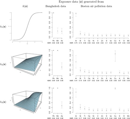
Median (25%, 75%) of the PIPs from BKMR with component-wise variable selection, across 300 simulated datasets for each of three true  functions. The vector of exposure data
  was generated either based on the Bangladesh data with
  mixture components, where the truly associated components were Pb for
  , and Pb and Mn for
  and
and  ; or based on the Boston air pollution data with
  mixture components, where the truly associated components were Al for
  , and Al and Cu for
  and
and  . The proportion of simulation iterations for which each mixture component had
  -value <0.05 under the garrote test for KMR is printed below the
  -axis.
  ;
;  ;
;  ;
;  ;
;  ;
;  ;
;  ;
;  ;
;  ;
;  ;
;  ;
;  carbon;
  ;
;  ;
;  .
.
We considered several exposure-response functions  that varied depending on the number of pollutants included, the degree of correlation of the included pollutants, and the shape of the function. We first considered three
  that depended on just one or two of the pollutants (Figure 1): a non-linear function of
  (
( ), a linear function with main effects of
  and
and  and their interaction (
 ), and a non-linear function of both
  and
and  with a synergistic interaction between them (
 ). We considered a scenario where the two included pollutants in
  and
and  were essentially uncorrelated (Mn, Pb for the Bangladesh dataset [
 ]; Al, Cu for the Boston dataset [
 ]) as well as a scenario where the two pollutants were more highly correlated (Mn, As for the Banladesh dataset [
 ]; Al, Ca for the Boston dataset [
 ]). Finally, to evaluated BKMR under a more complex setting with a larger number of mixture components, we considered two functions that included 6 of the 13 components from the Boston air pollution dataset:
 |
(3.1) |
 |
(3.2) |
These two functions are the same, except that  does not include any very highly correlated pollutants (the largest correlation is 0.49 between Al and S), whereas
  includes both Al and Si, which have a correlation of 0.87. Because these higher-dimensional
  require more power to detect, we halved the residual standard deviation (SD)
  when compared with the simulation studies for
  .
.
Models. First, we fit KMR using a frequentist approach (Liu and others, 2007), both without (KMR) and with (KMR-vs) variable selection. To conduct the variable selection, we applied the garrote KMR test from Maity and Lin (2011) to each component  (
( ) sequentially, and then re-fit the KMR including only those components with
  . Secondly, we fit three BKMR models: a model without variable selection (BKMR), a model with component-wise variable selection (BKMR-vs), and for the
  components exposure dataset, a model with hierarchical variable selection (BKMR-hvs). For BKMR-hvs, we defined the component groups
  (shown in Figure 2) based on knowledge of Boston air pollution sources. The within-group correlations ranged from 0.68 to 0.87 in
  and from 0.45 to 0.8 in
  (Figure 1 of supplementary material available at Biostatistics online). We ran each MCMC sampler (described in Section B of supplementary material available at Biostatistics online) for 10 000 iterations and kept the last 5000 samples. Finally, to quantify the optimal performance achievable if the true pollutants included in the
  function were known, we considered an “oracle” model. For
  , we fit a generalized additive model (GAM) including only
  , modeled using penalized splines, and a thin-plate regression basis (Wood, 2006); for
  , we fit a linear model with
  ,
,  , and the interaction term
  ; for
; for  we fit a GAM including a bivariate smooth function of
  and
and  ; and for
  and
and  we fit a GAM including independent bivariate smooth functions of the truly included pollutants in equations (3.1) and (3.2), respectively.
Fig. 2.
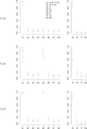
Median (25%, 75%) of the PIPs from BKMR with hierarchical variable selection, across 300 simulated datasets for each of three true  functions. Exposure data
  were generated based on the Boston air pollution data with
  mixture components categorized within eight groups. The truly associated components were Al (one of four pollutants in group 1) for
  , and Al and Cu (sole pollutant in group 5) for
  and
and  . Plots on left show the PIPs for each group, and plots on the right show the conditional PIPs for the components in group 1 given that group 1 was included in the model.
3.2. Results
Estimating the exposure-response function. We first evaluated the ability of each approach to estimate the subject-specific mixture effects  . Here we focus on results for the univariate and bivariate exposure-response functions under the scenario of uncorrelated exposures (Table 1); the relative performance of the methods for the other scenarios was similar. The approaches with variable selection (KMR-vs, BKMR-vs, and BKMR-hvs) each performed comparably to the oracle model (and outperformed the corresponding models without variable selection) in estimating the
  for the Bangladesh (
 ) exposure dataset. For the Boston (
 ) air pollution dataset, the Bayesian variable selection approaches outperformed all of the other methods (except the oracle model) for each
  . Across all scenarios, the Bayesian approaches were better able to capture the uncertainty in the
  when compared with the corresponding frequentist methods, achieving posterior SD estimates that were close to the empirical standard errors and interval coverage closest to the nominal (95%) level. KMR-vs had especially poor coverage, particularly for the
  scenarios, suggesting that the two-stage approach to estimating the exposure-response function does not fully account for uncertainty due to variable selection.
Table 1.
Performance of estimated subject-specific mixture effects,  across
  simulated datasets for each of three true exposure-response functions
  and two exposure generating models (
 )
)
Regression of  on on  |
Uncertainty |
|||||
|---|---|---|---|---|---|---|
| Intercept | Slope |

|
SD
|
SE | Cvg. | |

| ||||||

| ||||||
| Oracle |

|

|

|

|

|

|
| KMR |

|

|

|

|

|

|
| KMR-vs (297) |

|

|

|

|

|

|
| BKMR |

|

|

|

|

|

|
| BKMR-vs |

|

|

|

|

|

|

| ||||||
| Oracle |

|

|

|

|

|

|
| KMR |

|

|

|

|

|

|
| KMR-vs |

|

|

|

|

|

|
| BKMR |

|

|

|

|

|

|
| BKMR-vs |

|

|

|

|

|

|

| ||||||
| Oracle |

|

|

|

|

|

|
| KMR |

|

|

|

|

|

|
| KMR-vs |

|

|

|

|

|

|
| BKMR |

|

|

|

|

|

|
| BKMR-vs |

|

|

|

|

|

|

| ||||||

| ||||||
| Oracle |

|

|

|

|

|

|
| KMR |

|

|

|

|

|

|
| KMR-vs (273) |

|

|

|

|

|

|
| BKMR |

|

|

|

|

|

|
| BKMR-vs |

|

|

|

|

|

|
| BKMR-hvs |

|

|

|

|

|

|

| ||||||
| Oracle |

|

|

|

|

|

|
| KMR |

|

|

|

|

|

|
| KMR-vs (295) |

|

|

|

|

|

|
| BKMR |

|

|

|

|

|

|
| BKMR-vs |

|

|

|

|

|

|
| BKMR-hvs |

|

|

|

|

|

|

| ||||||
| Oracle |

|

|

|

|

|

|
| KMR |

|

|

|

|

|

|
| KMR-vs (298) |

|

|

|

|

|

|
| BKMR |

|

|

|

|

|

|
| BKMR-vs |

|

|

|

|

|

|
| BKMR-hvs |

|

|

|

|

|

|
Summary measures were obtained by regressing the estimated  on the true
  and reporting the average intercept, slope, and
  across simulation iterations; uncertainty measures were obtained by averaging over the uncertainty measures for the
  at each iteration and then averaging across all iterations. “SD” denotes the empirical standard error of the estimated
  “SE” denotes the estimated standard error or posterior SD of the
  and “Cvg.” denotes the proportion of times that the 95% confidence intervals or posterior credible intervals covered the true
  . Note that for some iterations no variables satisfied
  under the garrote kernel test and so KMR-vs was not applicable; the number of iterations for which KMR-vs was fit is given in parentheses beside the method name.
Identifying important mixture components. We next evaluated the ability of the methods to identify which mixture component(s) were included in  . Figure 1 shows, for the univariate and bivariate exposure-response functions
  –
– under the scenario of uncorrelated exposures, the median (IQR) for the posterior inclusion probabilities (PIPs) under BKMR-vs, as well as the proportion of iterations for which each component was identified as statistically significant under the garrote KMR test. For the Bangladesh (
 ) dataset, the garrote test achieved high power and the nominal type I error rate, and BKMR-vs was able to distinguish between the important versus unimportant components. For the Boston (
 ) dataset, the approaches were able to identify Cu, a component whose correlation with the other pollutants ranged from 0.13 to 0.29, as important in the scenarios where it was included in
  . On the other hand, for Al, a component highly correlated with several others (
 with Si, 0.7 with Ti, and 0.68 with Ca), the garrote test had lower power and had inflated type I errors with its correlated exposures, especially Si. For BKMR-vs, while the PIPs remained higher for Al than for its correlated exposures, Si also had higher PIPs relative to the other, unimportant components. Compared with the uncorrelated scenario, when the two pollutants included in
  and
and  were more highly correlated, the PIPs remained similar or were reduced (cf. Figure 2 of supplementary material available at Biostatistics online to Figure 1). For the higher-dimensional
  and
and  , BKMR-vs was generally able to distinguish the truly associated pollutants from the unassociated pollutants (Figure 2 of supplementary material available at Biostatistics online).
Figure 2 shows the PIPs for each group (i.e. the posterior mean of the group indicators  ), as well as the conditional PIPs for the components of group
  (i.e. the posterior mean of
  ) for
) for  –
– under the scenario of uncorrelated exposures (results for the other scenarios are in Figure 3 of supplementary material available at Biostatistics online). Across all scenarios, there is a clear separation between the PIPs for the groups that included one of the components that was truly predictive of health versus those that did not. In addition, for the truly associated pollutants within a multi-pollutant group (group
  under
under  –
– , group
  under
under  and
and  ), the group-specific PIPs were considerably larger than the corresponding component-specific PIPs obtained from BKMR-vs. This suggests that by incorporating the structure of the mixture into the model, BKMR-hvs achieves greater power to detect important components in the high correlation setting.
Within the multi-pollutant groups, the truly important components had higher conditional PIPs than the unimportant components. In the scenarios where the exposure-response function did not include correlated components, BKMR-hvs was better able to distinguish the important from the unimportant components when compared with BKMR-vs. When two pollutants from the same group were included in the exposure-response function, there was considerable variability in the conditional PIPs across simulation repetitions (see  ,
,  , and
, and  in Figure 3 of supplementary material available at Biostatistics online). In particular, for each generated dataset, usually one of the two important pollutants within the group had a high conditional PIP while the other pollutants in the group had much lower PIPs. This occurs because the hierarchical variable formulation (Section 2.3) assumes that only one pollutant from each group is included in the exposure-response function. Although this assumption may seem restrictive in that BKMR-hvs is not able to detect independent (or joint) effects of highly correlated pollutants within a group, such effects are typically not well-identified from the data in practice. For example, for BKMR-vs under
  , Al was identified as important using a threshold of 0.75 (i.e. had PIPs exceeding 0.75) in 59% of simulation repetitions, and Si was identified in 30% of repetitions, but both pollutants were simultaneously identified as important in only 3% of repetitions.
4. Application to a study of metals mixtures and neurodevelopment in Bangladesh
Preliminary data from 375 children (ages 1–4 years) were collected as part an ongoing study of metal exposures and neurodevelopment in Bangladesh (NIEHS grant P42 ES016454). A primary outcome ( ;
;  ) is the (
 -scored) motor composite score (MCS), a summary measure of psychomotor development derived as the sum of the fine and gross motor subscales from the Bayley Scales of Infant and Toddler Development (Bailey, 2005). Prenatal exposures (
 ) to As, Mn, and Pb (log transformed) were measured in umbilical cord blood. Exposure levels of Pb and Mn were uncorrelated, and As was inversely correlated with Pb (cor:
  ) and positively correlated with Mn (cor: 0.58). Covariates (
 ) consisted of gender, age in months at time of neurodevelopmental assessment (modeled using natural cubic splines with 3 degrees of freedom [df]), mother's education, mother's IQ (spline terms with 3 df), an indicator variable for which of two clinics the child visited, and HOME score (a proxy for socioeconomic status).
As a preliminary analysis, we fit linear regression models, adjusted for the covariates  . In single-metal models that included As, Mn, and Pb one at a time, as well as in a multi-metal model that included linear main effects of each metal concurrently, none of the metals were significantly associated with MCS (Table 1 of supplementary material available at Biostatistics online). To evaluate potential interaction among the three metals, we conducted an
  test to compare the fit of the multi-metal model including just main effects of each metal to the larger model that also contained the three pairwise interactions (
 ), and to the saturated model that additionally contained the three-way interaction term (
 ). Taken together, these results suggested little evidence of an exposure-response association, in the restrictive setting of linear and additive associations.
We then applied BKMR with component-wise variable selection to estimate the joint association of As, Mn, and Pb with MCS in a flexible way, without the need to specify a priori the form of the exposure-response function. We ran the MCMC sampler (described in Section B of supplementary material available at Biostatistics online) for 25 000 iterations after a burn in of 25 000 and every fifth sample was kept for inference. The estimated PIPs were 0.68 for Pb, 0.73 for Mn, and 0.77 for As. Figure 3 shows the estimated relationship of Mn and As with MCS for Pb fixed at its median value. This plot suggests an inverted  -shaped relationship for Mn with MCS, but only at middle levels of As exposure. Similar patterns occurred at other levels of Pb (Figure 4 of supplementary material available at Biostatistics online). To confirm that our finding of a non-additive and non-linear exposure-response function for Mn and As under BKMR was real and not an artifact of the method, we subsequently fit a GAM with the same covariates as above, together with a main effect of Pb and separate smooth functions (thin-plate regression splines; smoothing parameter estimated using generalized cross validation) of Mn at each tertile of As exposure. We found a similar inverted
  relation between Mn and MCS, and the smooth term was only statistically significant at the second tertile of As (Figure 5 of supplementary material available at Biostatistics online).
Fig. 3.
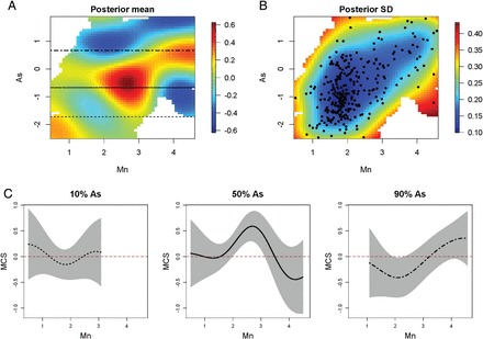
Relationship of manganese (Mn) and arsenic (As) with the MCS, for lead (Pb) fixed at its median. (A) Posterior mean of the bivariate exposure-response function  for Mn and As. Horizontal lines correspond to the 10th, 50th, and 90th percentiles of As. (B) Posterior SD of
  . Points correspond to the observed data points. (C) Relationship of Mn with MCS at three levels of As together with pointwise 95% credible intervals.
5. Application to a toxicology study of air pollution mixtures and hemodynamics
We considered data from a toxicology study, in which 13 dogs were repeatedly exposed for 5 h to either concentrated ambient particles (CAPs) or filtered air in a cross-over protocol (Bartoli and others, 2009). Previous analyses found elevated blood pressure associated with CAPs exposure; our goal was to identify whether particular component(s) of the CAPs are responsible for these observed effects. Let  be the average heart rate for dog
  at exposure occasion
  ,
,  be indicator variables for CAPs versus filtered air exposure and for the other experimental conditions (whether the exposure occurred post-occlusion or after prazosin was administered), and
  be the vector of elemental concentrations for the CAPs components, where we considered the same pollution constituents as in our simulation study (Section 3). Because in this small subsample of days K, Cu, and Mn were also highly correlated with Al, Si, Ti, and Ca (all pairwise correlations among these seven pollutants were
  0.76), we included these additional elements in group
  . After removing several outliers in the elemental concentrations, the dataset consisted of
  dog-exposures.
We began by fitting linear mixed models (LMMs) of the CAPs components with dog-specific random intercepts, adjusted for the covariates  . In models that included each component separately, all of the pollutants in
  (except Cu) had statistically significant associations with elevated heart rate (none of the other components were associated). However, these associations were no longer significant in the multi-pollutant LMM that included all of the constituents concurrently, and for three of these components the direction of the association was reversed (Table 2 of supplementary material available at Biostatistics online).
Because of the longitudinal cross-over design of the study, we extended the BKMR models described in Section 2 to include random (dog-specific) intercepts. We fit BKMR models including all of the 13 pollutants with both component-wise and hierarchical variable selection. We ran the MCMC samplers (described in Section B of supplementary material available at Biostatistics online) for 25 000 iterations after a burn in of 25 000 and every fifth sample was kept for inference. We did not find evidence of non-linearity or interaction, so here we focus on the variable selection results. Analogous to the null results from the multi-pollutant LMM, under the component-wise BKMR model we found that each component had a PIP of  ; in contrast, under the hierarchical selection approach group
  had a PIP of 0.79 (Figure 4). Given the strong correlations among components in this group, the data did not strongly favor one constituent over the others as driving the observed association between heart rate and this group of elements (the conditional inclusion probabilities ranged from 0.04 for Cu to 0.36 for Si). In this case, our strong preference is the hierarchical variable selection approach, as it accurately conveys that there is a group of elements that are associated with the outcome but that the data cannot definitively identify a constituent driving this association.
Fig. 4.
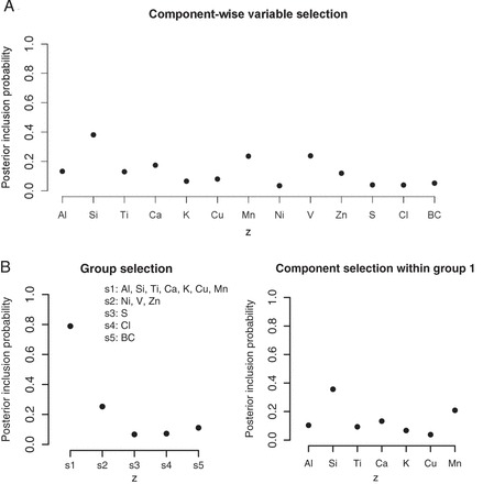
PIPs for the toxicology application estimated from BKMR with component-wise variable selection (A) and hierarchical variable selection (B). Left panel shows group-specific PIPs and right panel shows conditional inclusion probabilities for the components in group 1.
6. Discussion
We have proposed BKMR as a new approach to estimate the health effects of multi-pollutant mixtures. Our simulation studies highlighted two main advantages of BKMR over existing frequentist approaches. First, by conducting variable selection and health effect estimation simultaneously the Bayesian approach was able to more fully capture the uncertainty in the exposure-response function due to selecting which mixture components to include in the model. Secondly, the garrote KMR test (Maity and Lin, 2011) had low power to detect important mixture components in the setting of multiple highly correlated exposures. Because this procedure tests for the effect of a variable  by conducting a score-based test of the null hypothesis
  , if the null model already includes a variable that is highly correlated with a truly important variable, then there may not be enough information remaining in the data to detect the true association. Our hierarchical variable selection approach addresses this issue by allowing one component from a group of highly correlated components to enter into the model at a time.
We focused on the Gaussian kernel, although other kernels could be considered. In simulation studies of KMR with  having a complicated functional form, Liu and others (2007) found the Gaussian kernel to outperform both the quadratic and ridge regression kernels. Our simulation studies demonstrated that the Gaussian kernel performed well across a range of plausible exposure-response functions for environmental health applications. In future work, Bayesian model selection could be applied to formally evaluate the choice of kernel.
The larger set of 13 predictors in our simulation studies is not particularly large relative to many high-dimensional application areas, such as statistical genomics and other ’omics settings. A few environmental health studies have considered exposures in the hundreds, but these have typically been conducted with the goal of screening for the most important exposures (Patel and others, 2010) or classes of exposures (Kioumourtzoglou and others, 2013), rather than fully characterizing the form of the exposure-response surface. Thirteen pollutants represents a typical number considered in PM elemental composition studies focusing on the exposure-response relationship. Computationally, the dimension of the exposure vector is not a limiting factor in these models, as the dimension of the exposures gets reduced into the pairwise distance measures contained in the kernel matrix.
It is well known that Bayesian variable selection methods can be highly sensitive to the specification of the mixture prior. In our applications, we found that changing the distribution of the slab part of the prior ( in equation (2.3)) led to changes in the values of the PIPs; however, their relative ordering was preserved across prior specifications. This issue is analogous to the variable importance measures produced by a random forests analysis, whose absolute magnitude can be sensitive to tuning parameters, but that the rank ordering of these importance scores across the multiple pollutants are relatively stable (Liaw and Wiener, 2002).
To our knowledge, this work represents the first instance of incorporating structure among pollutants within the kernel machine framework. By grouping highly correlated pollutants together, our approach had greater power to detect associations between these pollutants and health. In some situations, such groups may represent pollution sources, but not in the (relatively) small toxicology application we considered. In future work, we will consider more complex structures, such as overlapping groups, that likely occur in air pollution source apportionment settings. Another useful extension of the model would be to account for exposure measurement error, which may arise from known error in the measured concentrations, or from uncertainty in estimated source contributions from a source apportionment model (Kioumourtzoglou and others, 2014) or in predicted exposures obtained from a spatial model addressing misalignment of the pollutant and outcome data (Gryparis and others, 2009; Szpiro and others, 2011; Szpiro and Paciorek, 2013).
Supplementary material
Supplementary material is available online at http://biostatistics.oxfordjournals.org.
Funding
This work was supported by a grant from the Health Effects Institute; National Institutes of Health [ES007142, ES016454, ES000002, ES014930, ES013744, ES017437, ES015533, ES022585]; and U.S. Environmental Protection Agency (EPA) [83479801]. Its contents are solely the responsibility of the grantee and do not necessarily represent the official views of the US EPA. Further, US EPA does not endorse the purchase of any commercial products or services mentioned in the publication.
Supplementary Material
Acknowledgement
Conflict of Interest: None declared.
References
- Bailey N. (2005). Bayley Scales of Infant and Toddler Development, Administration Manual, 3rd edition. San Antonio, TX: Harcourt Assessment. [Google Scholar]
- Bartoli C. R., Wellenius G. A., Diaz E. A., Lawrence J., Coull B. A., Akiyama I., Lee L. M., Okabe K., Verrier R. L., Godleski J. J. (2009). Mechanisms of inhaled fine particulate air pollution-induced arterial blood pressure changes. Environmental Health Perspectives 117(3), 361–366. [DOI] [PMC free article] [PubMed] [Google Scholar]
- Billionnet C., Sherrill D., Annesi-Maesano I. (2012). Estimating the health effects of exposure to multi-pollutant mixture. Annals of Epidemiology 22(2), 126–141. [DOI] [PubMed] [Google Scholar]
- Breiman L. (2001). Random forests. Machine Learning 45(1), 5–32. [Google Scholar]
- Carlin D. J., Rider C. V., Woychik R., Birnbaum L. S. (2013). Unraveling the health effects of environmental mixtures: an NIEHS priority. Environmental Health Perspectives 102(1), A6–A8. [DOI] [PMC free article] [PubMed] [Google Scholar]
- Claus Henn B., Schnaas L., Ettinger A. S., Schwartz J., Lamadrid-Figueroa H., Hernández-Avila M., Amarasiriwardena C., Hu H., Bellinger D. C., Wright R. O., Téllez-Rojo M. M. (2012). Associations of early childhood manganese and lead coexposure with neurodevelopment. Environmental Health Perspectives 120(1), 126–131. [DOI] [PMC free article] [PubMed] [Google Scholar]
- Cristianini N., Shawe-Taylor J. (2000). An Introduction to Support Vector Machines and Other Kernel-Based Learning Methods. Cambridge, UK: Cambridge University Press. [Google Scholar]
- Gennings C., Sabo R., Carney E. (2010). Identifying subsets of complex mixtures most associated with complex diseases: polychlorinated biphenyls and endometriosis as a case study. Epidemiology 21(Suppl 4), S77–S84. [DOI] [PubMed] [Google Scholar]
- George E., McCulloch R. (1993). Variable selection via Gibbs sampling. Journal of the American Statistical Association 88(423), 881–889. [Google Scholar]
- Gryparis A., Paciorek C. J., Zeka A., Schwartz J., Coull B. A. (2009). Measurement error caused by spatial misalignment in environmental epidemiology. Biostatistics 10(2), 258–274. [DOI] [PMC free article] [PubMed] [Google Scholar]
- Hu H., Shine J., Wright R. O. (2007). The challenge posed to children's health by mixtures of toxic waste: the Tar Creek Superfund site as a case-study. Pediatric Clinics of North America 54(1), 155–75, x. [DOI] [PMC free article] [PubMed] [Google Scholar]
- Kioumourtzoglou M.-A., Coull B. A., Dominici F., Koutrakis P., Schwartz J., Suh H. (2014). The impact of source contribution uncertainty on the effects of source-specific pm2.5 on hospital admissions: a case study in Boston, MA. Journal of Exposure Science and Environmental Epidemiology 24(4), 365–371. [DOI] [PMC free article] [PubMed] [Google Scholar]
- Kioumourtzoglou M.-A., Zanobetti A., Schwartz J. D., Coull B. A., Dominici F., Suh H. H. (2013). The effect of primary organic particles on emergency hospital admissions among the elderly in 3 US cities. Environmental Health 12(19), 20. [DOI] [PMC free article] [PubMed] [Google Scholar]
- Liaw A., Wiener M. (2002). Classification and regression by randomforest. R News 2, 18–22. http://CRAN.R-project.org/doc/Rnews/. [Google Scholar]
- Linkletter C., Bingham D., Hengartner N., Higdon D., Kenny Q. Y. (2006). Variable selection for Gaussian process models in computer experiments. Technometrics 48(4), 478–490. [Google Scholar]
- Liu D., Lin X., Ghosh D. (2007). Semiparametric regression of multidimensional genetic pathway data: least-squares kernel machines and linear mixed models. Biometrics 63(4), 1079–1088. [DOI] [PMC free article] [PubMed] [Google Scholar]
- Maity A., Lin X. (2011). Powerful tests for detecting a gene effect in the presence of possible gene-gene interactions using garrote kernel machines. Biometrics 67(4), 1271–1284. [DOI] [PMC free article] [PubMed] [Google Scholar]
- Patel C. J., Bhattacharya J., Butte A. J. (2010). An environment-wide association study (EWAS) on type 2 diabetes mellitus. PLOS ONE 5. Article Number: e10746. [DOI] [PMC free article] [PubMed] [Google Scholar]
- Savitsky T., Vannucci M., Sha N. (2011). Variable selection for nonparametric Gaussian process priors: models and computational strategies. Statistical Science 26(1), 130–149. [DOI] [PMC free article] [PubMed] [Google Scholar]
- Szpiro A. A., Paciorek C. J. (2013). Measurement error in two-stage analyses, with application to air pollution epidemiology. Environmetrics 24(8), 501–517. [DOI] [PMC free article] [PubMed] [Google Scholar]
- Szpiro A. A., Sheppard L., Lumley T. (2011). Efficient measurement error correction with spatially misaligned data. Biostatistics 12(4), 610–623. [DOI] [PMC free article] [PubMed] [Google Scholar]
- Thomas D. C., Witte J. S., Greenland S. (2007). Dissecting effects of complex mixtures: who's afraid of informative priors? Epidemiology 18(2), 186–190. [DOI] [PubMed] [Google Scholar]
- Tibshirani R. (1994). Regression shrinkage and selection via the lasso. Journal of the Royal Statistical Society, Series B 58, 267–288. [Google Scholar]
- Wood S. N. (2006). Generalized Additive Models: An Introduction with R. Boca Raton, FL: CRC Press. [Google Scholar]
- Zou F., Huang H., Lee S., Hoeschele I. (2010). Nonparametric bayesian variable selection with applications to multiple quantitative trait loci mapping with epistasis and gene-environment interaction. Genetics 186(1), 385–394. [DOI] [PMC free article] [PubMed] [Google Scholar]
Associated Data
This section collects any data citations, data availability statements, or supplementary materials included in this article.