Assessment of critical exposure and outcome windows in time-to-event analysis with application to air pollution and preterm birth study

Abstract

In reproductive epidemiology, there is a growing interest to examine associations between air pollution exposure during pregnancy and the risk of preterm birth (PTB). One important research objective is to identify critical periods of exposure and estimate the associated effects at different stages of pregnancy. However, population studies have reported inconsistent findings. This may be due to limitations from the standard analytic approach of treating PTB as a binary outcome without considering time-varying exposures together over the course of pregnancy. To address this research gap, we present a Bayesian hierarchical model for conducting a comprehensive examination of gestational air pollution exposure by estimating the joint effects of weekly exposures during different vulnerable periods. Our model also treats PTB as a time-to-event outcome to address the challenge of different exposure lengths among ongoing pregnancies. The proposed model is applied to a dataset of geocoded birth records in the Atlanta metropolitan area between 1999–2005 to examine the risk of PTB associated with gestational exposure to ambient fine particulate matter m in aerodynamic diameter (PM). We find positive associations between PM exposure during early and mid-pregnancy, and evidence that associations are stronger for PTBs occurring around week 30.

1. Introduction

Epidemiological evidence on the health effects of outdoor air pollution plays an important role in setting regulatory standards and protecting public health. This has led to development of statistical modeling approaches motivated by specific analytic challenges arising from different health outcomes and study designs. There exists increasing interest in examining the potential link between a mother's exposure to air pollution during pregnancy and the risk of adverse birth outcomes. Preterm birth (PTB), defined as gestational age at delivery of <37 weeks, is the leading cause of neonatal mortality and morbidity (Goldenberg and others, 2008; Saigal and Doyle, 2008). In addition to health care expenses, PTB is also associated with long-term physical, cognitive, and developmental problems (Moster and others, 2008).

This paper describes a flexible modeling approach for estimating associations between PTB and a time-varying environmental exposure, such as air pollution, during pregnancy. The proposed model is motivated by the need to address two scientific questions of significant interest in environmental reproductive epidemiology. First, is PTB associated with critical gestational exposure periods that may correspond to specific stages of fetal development? For example, is high exposure that occurs during the first trimester more adverse than that occurring during the third trimester? Second, do exposures have different impacts on different outcome periods? For example, are ongoing pregnancies more vulnerable to the acute effect of air pollution as they progress closer to 37th week? There are differences in risk factors for earlier (e.g. weeks) versus later PTB (e.g. 34–36 weeks) and air pollution may only increase the risk of PTB occurring at certain stages of pregnancy. These findings on exposure and outcome windows can potentially provide crucial information on the biological mechanisms by which air pollution affects adversely on birth outcomes, as well as help develop public health messages to minimize harmful exposures during pregnancies.

The hypothesis on critical exposure windows can be examined by considering time-varying coefficients across gestational length; while the hypothesis on outcome windows considers PTB as a spectrum of outcomes, defined by gestational week at birth, rather than as a dichotomous outcome (Suh and others, 2009). We propose an approach to address these two scientific questions simultaneously by treating gestational age as time-to-event data (Chang and others, 2013). Here, we consider a discrete-time domain in weeks because gestational age is typically reported as the number of completed weeks. We then model the hazard rate at week as a function of weekly air pollution exposure following conception until week and allow the exposure effects to vary both across exposure weeks, as well as across outcomes weeks. The main advantage of a time-to-event approach is that it can effectively accommodate the differences in exposure length among pregnancies of different gestational ages. By considering PTB at different gestational ages, we are also able to distinguish between risks associated with early versus late PTB, which is important because each additional week of gestation during this critical time period leads to better health outcomes for the child.

The idea of estimating time-varying effects of time-varying exposures in a health model is similar to the distributed lag approach commonly used in time series studies of air pollution and health to examine associations between daily adverse health outcome counts and exposure to air pollution on the previous days (Schwartz, 2000). To stabilize estimation and borrow information across exposure days, several constraints have been proposed, including penalized splines (Zanobetti and others, 2000), Gaussian processes (Heaton and Peng, 2012), autoregressive priors (Fahrmeir and Knorr-Held, 1997), and hierarchical structures (Welty and others, 2009). Recently, the distributed lag model has been applied to PTB for identifying critical exposure window by Warren and others (2012). In this paper, we extend previous work by considering distributed exposures that vary in two dimensions (i.e. exposure weeks and outcome weeks). Specifically, we allow the associations between exposure at each week of pregnancy and the risk of PTB to vary over the course of the pregnancy. Our model is also related to survival models that consider time-dependent exposures or time-varying (dynamic) effects (McKeague and Tighiouart, 2000; Haneuse and others, 2008; Buchholz and Sauerbrei, 2011; He and others, 2012); however, to our knowledge no method has been developed to examine whether the time-varying effects differ across outcome periods.

The proposed model is applied to a birth cohort in the Atlanta metropolitan area. We examines association between PTB and ambient fine particulate matter m in aerodynamic diameter (PM). PM is a complex mixture of solid and liquid particles suspended in the atmosphere, and has been linked to increased risks of various adverse health outcomes (US EPA, 2009). The remainder of this paper is organized as follows. Section 2 describes the motivating Atlanta air pollution and birth record data. Section 3 describes the distributed exposure discrete-time survival model for PTB. In Section 4, we describe a simulation study that evaluates the proposed model's performance in identifying exposure and outcome windows. Results from the health analysis are given in Section 5. Finally, discussion and future work appear in Section 6.

2. Data

Birth records were obtained from the Office of Health Research and Policy, Georgia Division of Public Health. We included only singleton births without major structural birth defects conceived from January 1, 1999 to December 31, 2005. Gestational age in weeks was determined by the reported date of last menstrual period. We defined the study population using conception dates instead of birth date to avoid fixed-cohort bias when examining time-varying exposures (Strand and others, 2011b). Maternal residential address at delivery was geocoded to the census blockgroup level and this study included geocoded births within the 5-county Atlanta metropolitan area (Clayton, Cobb, DeKalb, Fulton, and Gwinnett). We restricted the analysis to Hispanic, non-Hispanic black, non-Hispanic white, and Asian mothers between the age of 15–44. We only considered PTB that reached at least 27 weeks of gestation.

Daily measurements of ambient PM concentrations were obtained from 14 air quality monitors within the study region. Daily PM concentrations showed strong spatial homogeneity, with a median between-monitor correlation of 0.85. We also obtained daily average temperature from the National Climatic Data Center, and census tract-level percent household below poverty from the US 2000 Census. Each geocoded pregnancy was linked to the closest PM monitor within a 10 km radius to minimize spatial exposure measurement error (median distance of 5.15 km). We defined the exposure for week as the average pollution levels on the date that week was completed and the 6 days leading up to it. Weekly average temperature was defined similarly. Daily air pollution measurements contained missing values (2.5%). For weeks without any PM measurements, the averages of the weeks before and after were used. Births with 2 or more consecutive missing weeks were excluded.

3. Methods

3.1. Distributed exposure time-to-event model for PTB

We view gestational age as discrete-time survival data where each pregnancy enters the risk set at the 27th week. Full-term births of at least 37 weeks are censored at 36 weeks because they are no longer at risk of being preterm. Let denote the hazard rate of birth during outcome (at-risk) window week for pregnancy . Denote the average air pollution exposure for pregnancy during gestational week where . We model the discrete event hazard rate using probit regression,

(3.1)

where is the standard normal distribution function, is the regression coefficients for the vector of confounders , and denotes the baseline hazard function specified using indicator variables for each outcome week . Therefore, the model should only consider outcome weeks with enough births such that the baseline hazard can be estimated well. We refer to model (3.1) as a distributed exposure time-to-event model because it allows the air pollution effects to vary across exposure and outcome weeks. Specifically, the parameter of interest represents the effect of exposure during week on the risk of PTB at gestational age . Note that for a given outcome week , is defined only for as future exposures cannot affect PTB risk at week .

To estimate , we wish to borrow information across exposure weeks and outcome weeks by assigning prior structure to the vectors of parameters , . Besides stabilizing coefficient estimation, this is also motivated by the temporal correlation in weekly ambient air pollution exposures and potential misclassification of gestational age. In total, the health model contains weekly pollutant effects and can be visualized in a matrix below by stacking horizontally,

(3.2)

where row indices denote the outcome weeks and column indices denote the exposure weeks. We wish to encourage smoothing in both the rows and the columns of the above matrix.

Let denote the first to th element of vector . We propose the following dynamic Gaussian process prior:

(3.3)

where and is a covariance matrix. The degree of smoothing across outcome weeks is controlled by parameter . Specifically, the correlation between exposure effects during week across outcome weeks and is given by . Note that we anchor the model at gestational week 36 because by working backward in gestational age, the model naturally handles the staircase coefficient structure in . The degree of smoothing across exposure weeks (within each vector ) is determined by , which we assume to have the form with . The above dynamic specification results in a common marginal variance of each given by . Inference is carried out in a Bayesian framework. Estimation details and R code (R Core Team, 2014) are provided in supplementary material available at Biostatistics online.

3.2. Estimating cumulative effects

There are several advantages associated with estimating all combinations of exposure and outcome windows jointly. First, the risks associated with different long-term and short-term exposure metrics can be derived by considering different summations of . This is similar to interpreting cumulative risks in a distributed lag model. For example, the risk associated with exposure across the first trimester (conception until gestational week 13) on PTB at a particular outcome window can be estimated as . The standard error for can be derived either through the delta method or Bayesian inference via posterior samples. Time-varying lagged exposures can also be examined. For example, represents the risk due to air pollution exposures experienced 1-month prior at gestational age week .

Subsequently, can also be combined across different outcome windows. For example, under a fixed-effect meta-analysis framework, we can define the overall first trimester exposure effects across gestational week 27 until 36 as , where and is the corresponding variance–covariance matrix. We note that we do not sum over because it combines risks due to the same exposure that are conditioned on different baseline hazard and at different time points. Instead, we believe it is more intuitive to summarize the effect over outcome weeks as an average, weighted by its uncertainty. The ability to estimate air pollution risks across different gestational ages is particularly useful for examining whether the impacts of air pollution exposure differ between early and late PTBs.

4. Simulation study

We carried out a simulation study to evaluate the benefits of borrowing information across exposure and outcome windows in a distributed exposure analysis. We generated 20 replicates of simulated air pollution exposures and gestational age for 50 000 births as follows. First, for each birth , we generated weekly exposures from a multivariate normal distribution with marginal means of 17.2 and marginal variances of 43. We assumed the correlation between weeks and to be . These values were chosen to reflect the temporal variability and correlation observed in the Atlanta data. Then gestational age for pregnancy was generated with probability where for . We estimated the baseline hazard function using the Atlanta birth record data. We allowed the gestational age of each birth to be subject to misclassification. Based on previous studies on the disagreement between gestational age defined using clinical estimate or last menstrual period (Mustafa and David, 2001), we assumed the error between observed and true gestational age to be at most 1, 2, and 3 weeks with probability 0.8, 0.1, and 0.1, respectively.

We considered 5 scenarios of different exposure and outcome windows. In Scenario 1, we assumed a fixed-length 13-week exposure window between gestational weeks 14–26 (second trimester). This effect is identical for all ongoing pregnancies during the entire at-risk window (weeks 27–36). In Scenario 2, we assumed a shorter 6-week exposure during weeks 14–21, common across all at-risk weeks. In Scenario 3, we assumed the 13-week exposure from Scenario 1 only has an effect for pregnancies early during the at-risk window. In Scenario 4, we assumed a 4-week lagged exposure that is common across all at-risk weeks. Finally, Scenario 5 assumed the lagged effect is only present for pregnancies that have reached gestational age 32. We assigned each non-zero , corresponding to an approximate 1.05 increase in hazard ratio per interquartile range (IQR) increase in weekly exposure.

• Scenario 1: For all , if .

• Scenario 2: For all , if .

• Scenario 3: For , if .

• Scenario 4: For all , if .

• Scenario 5: For , if .

For each simulated dataset, we fitted the time-to-event model with the following four covariance structure specifications for : (1) the proposed dynamic model, (2) an exchangeable model by setting that does not borrow information across outcome weeks, (3) an independent random effect model where that does not borrow information across both exposure and outcome weeks, and (4) a fixed prior structure ( and for all ) that assumes identical weekly exposure effects across outcome weeks. The fixed prior also represents an extension of the distributed lag model of Warren and others (2012) to a time-to-event setting.

Table 1 gives the relative changes in root mean-square error (RMSE), 95% posterior interval (PI) length, and changes in deviance information criterion (DIC) and effective degrees of freedom (pD) (Spiegelhalter and others, 2002). We found that the dynamic model consistently out-performed the independent and the exchangeable model in terms of RMSE and PI length. The gain in performance is greater for longer exposure window (Scenario 1). The difference between the dynamic and the exchangeable model is less pronounced for shorter fixed-length exposure windows (Scenario 2). Importantly, performance of the dynamic model does not degrade in situations where the exposure effects are only present for some outcome weeks (Scenarios 3 and 5). Finally, the dynamic model consistently results in smaller DIC and smaller effective degrees of freedom, which indicate improved model fit and the presence of additional shrinkage across outcome/exposure weeks.

Table 1.

Simulation study results for estimating weekly PM effects across outcome weeks: relative change in RMSE, length of PIs, and change in DIC and effective degrees of freedom (pD), averaged across simulated replicate datasets

	Exposure	Outcome	Prior	Relative	Relative
	weeks	weeks	structure	RMSE	PI length	DIC	pD
Scenario 1	14–26	27–36	Dynamic	Reference
			Independent	2.13 (0.17)	3.39 (0.16)	121 (19)	130 (12)
			Exchangeable	1.41 (0.08)	1.53 (0.09)	46 (11)	36 (12)
			Fixed	0.88 (0.04)	0.66 (0.04)	(10)	(3)
Scenario 2	14–19	27–36	Dynamic	Reference
			Independent	1.64 (0.13)	2.74 (0.26)	57 (15)	69 (5)
			Exchangeable	1.14 (0.09)	1.95 (0.23)	38 (14)	44 (6)
			Fixed	0.87 (0.07)	0.63 (0.06)	(9)	(5)
Scenario 3	14–26	27–31	Dynamic	Reference
			Independent	1.74 (0.13)	2.78 (0.28)	70 (16)	76 (7)
			Exchangeable	1.31 (0.16)	1.52 (0.32)	31 (13)	27 (14)
			Fixed	1.62 (0.12)	0.43 (0.06)	106 (21)	(6)
Scenario 4	4-wk lag	27–36	Dynamic	Reference
			Independent	1.34 (0.09)	2.75 (0.30)	23 (9)	46 (5)
			Exchangeable	1.32 (0.09)	2.63 (0.38)	21 (8)	45 (5)
			Fixed	1.13 (0.11)	0.41 (0.08)	(9)	(4)
Scenario 5	4-wk lag	31–36	Dynamic	Reference
			Independent	1.25 (0.09)	2.85 (0.45)	17 (10)	44 (6)
			Exchangeable	1.24 (0.13)	2.68 (0.61)	15 (7)	40 (9)
			Fixed	0.93 (0.08)	0.45 (0.08)	(6)	(5)

The standard deviations across replicate datasets are given in parentheses.

The fixed prior resulted in a large reduction in 95% PI length because it utilizes data from all outcome weeks. Compare with the dynamic prior, it under-performs when the exposure effects vary across outcome weeks (Scenarios 3 and 4). For Scenario 5, where the 4-week lag effects are only present during outcome weeks 31–36, the fixed and dynamic priors perform similarly, likely because there is considerable overlapping exposure effects across outcome weeks. Figure S1 of supplementary material available at Biostatistics online plot the estimated weekly effects, averaged across replicates, for outcome weeks 28, 32, and 36. Visually, Figure S1 of supplementary material available at Biostatistics online demonstrates the dynamic prior's ability to capture the underlying true effects, as well as the smoothing effect compared to the other priors.

We also compared the cumulative effects obtained from combining weekly effects to that estimated by first averaging weekly exposure over a pre-defined window. Specifically, we fitted a time-to-event model where the exposures were averaged across the known true at-risk and outcome windows. This corresponds to the standard exposure assessment approach taken by Chang (Reich, and others, 2012). This allows us to examine the model's performance associated with using weekly exposures when the true association spans across several weeks. Simulation results are given in Table S1 of supplementary material available at Biostatistics online. Compared with an analysis where the true exposure windows are known, the cumulative effects estimated by combining weekly effects were associated with a slight negative bias. This is likely due to shrinkage and the use of a Gaussian process to approximate the true step risk function. However, the dynamic model consistently out-performs the other 2 prior structures. Table S1 of supplementary material available at Biostatistics online also indicates that the use of averaged exposure can lead to larger estimation uncertainty.

To examine how the different models perform in detecting risk, we calculated the sensitivity and specificity (Table 2). The dynamic model has better sensitivity compared with the exchangeable and the independent prior structures. The dynamic model does suffer from a slightly reduced specificity compared with the exchangeable and the independent priors; however these false positives occur near the boundary of the true risk window and across outcome weeks. Finally, the dynamic prior out-performs the fixed prior in specificity, especially when the exposure weeks differ across outcome weeks (Scenarios 3). Table 2 also gives the empirical 95% PIs coverage probability. For the dynamic and fixed priors, coverage is slightly under due to the presence of exposure measurement error.

Table 2.

Simulation study results for the sensitivity and specificity of detecting a non-null weekly PM effects, averaged across replicates

	Exposure	Outcome	Prior			95% PI
	weeks	weeks	structure	Sensitivity	Specificity	coverage
Scenario 1	14–26	27–36	Dynamic	1.00 (0.00)	0.90 (0.03)	0.85 (0.03)
			Exchangeable	0.85 (0.04)	0.96 (0.02)	0.88 (0.03)
			Independent	0.16 (0.03)	0.99 (0.01)	0.98 (0.01)
			Fixed	1.00 (0.00)	0.85 (0.05)	0.78 (0.05)
Scenario 2	14–19	27–36	Dynamic	0.96 (0.04)	0.93 (0.03)	0.86 (0.03)
			Exchangeable	0.28 (0.08)	1.00 (0.00)	0.94 (0.02)
			Independent	0.06 (0.03)	1.00 (0.00)	0.98 (0.01)
			Fixed	1.00 (0.00)	0.89 (0.03)	0.77 (0.04)
Scenario 3	14–26	27–31	Dynamic	0.98 (0.02)	0.91 (0.03)	0.89 (0.04)
			Exchangeable	0.60 (0.21)	0.98 (0.02)	0.92 (0.04)
			Independent	0.03 (0.02)	1.00 (0.00)	0.99 (0.01)
			Fixed	0.95 (0.06)	0.69 (0.07)	0.54 (0.07)
Scenario 4	4-wk lag	27–36	Dynamic	0.70 (0.18)	0.94 (0.02)	0.84 (0.03)
			Exchangeable	0.03 (0.04)	1.00 (0.00)	0.94 (0.02)
			Independent	0.01 (0.02)	1.00 (0.00)	0.94 (0.02)
			Fixed	0.87 (0.11)	0.90 (0.04)	0.79 (0.04)
Scenario 5	4-wk lag	31–36	Dynamic	0.80 (0.19)	0.95 (0.03)	0.90 (0.03)
			Exchangeable	0.07 (0.12)	1.00 (0.00)	0.97 (0.01)
			Independent	0.02 (0.03)	1.00 (0.00)	0.97 (0.01)
			Fixed	0.99 (0.02)	0.91 (0.03)	0.86 (0.03)

The overall empircal coverage probability of the PI is also given. The standard deviations across replicate datasets are given in parentheses.

5. Analysis of the Atlanta Birth Cohort, 19992005

The study included 175 891 pregnancies (10.6% preterm). Weekly PM exposures, averaged across all pregnancies, were similar for weeks 1–37, ranging 17.1–. The variability in weekly exposures in terms of IQR was also similar across weeks, ranging from 7.34 to . This is due to the relatively small seasonal trend in the number of ongoing pregnancies in our study population. Weekly PM exposures showed moderate temporal correlation with a median lag-1 auto-correlation of 0.50 across pregnancies. For outcome weeks 27–36, the corresponding PTB numbers are 303, 320, 383, 439, 563, 830, 1291, 2362, 4134, and 8023. We fitted the distributed exposure time-to-event model with a dynamic prior for weekly exposures. The list of confounders included in the model and their associations are given in Section 2 of supplementary material available at Biostatistics online.

5.1. Results

For small probabilities, the Gaussian distribution function can be approximated by an exponential function: . The unadjusted hazard rates of PTB during outcome weeks 27–26 were <0.05. Therefore, to aid in the interpretation of probit regression coefficients, we present the posteriors of as the approximate relative risk (RR) of PTB due to a unit increase in the exposure. Here an RR of 1 indicates the covariate is not associated with PTB risk. Figure 1 shows the posterior means and 95% PI of the RRs associated with different exposure weeks by outcome weeks. The PI width decreases for later outcome weeks due to the increasing number of PTBs. Overall we found relatively smooth time-varying effects within each outcome week. Figure 2 shows the posterior probability of . There is evidence of positive associations with exposures occurring during between early and mid-pregnancy, and these associations are only present when an ongoing pregnancy was between weeks 28–31 (among very PTB). We also found weak evidence that late trimester 2 exposures were associated with PTB occurring after week 32 (late PTB). We also fitted the health data using the fixed prior. This resulted in a slight increase in DIC (1.7). Figure S3 of supplementary material available at Biostatistics online shows the posterior means and 95% PI's of the weekly exposure effects. While increased risks were found around exposure week 20, the effects were attenuated compared with that from the dynamic model, and none of the 95% PI excluded 1.

Fig. 1.

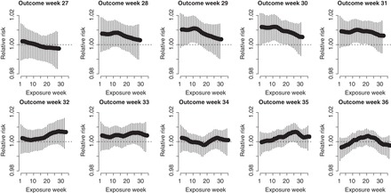
Posterior means and 95% PIs of the RRs for PTB associated with an IQR () increase in weekly PM exposure.

Fig. 2.

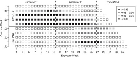
Posterior probabilities of weekly PM effects being greater than zero: .

We then examined cumulative effects as described in Section 3.2. Figure 3 shows the RR for PTB associated with different windows of exposure commonly utilized in the literature. We examined 3 time-invariant exposures: trimester 1 (weeks 1–13); trimester 2 (weeks 14–27); and the 4 weeks after conception. Given that an ongoing pregnancy completed gestational week , we also examined 3 time-varying exposures: cumulative (week 1 to ); trimester 3 (week 27 to ); and a 4-week lag (week -3 to ). The estimates are scaled by an IQR of the exposure metric across the study population given in Table 3. Based on the aggregated exposures, we found evidence of positive associations between PTB risk and PM levels during trimester 1 and trimester 2. These associations were also more pronounced for PTB occurring between 29 and 31 weeks.

Fig. 3.

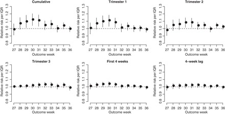
Posterior means and 95% PIs of the RRs for PTB per IQR increase in different metrics of exposure to PM. The IQR for the exposures are given in Table 3.

Table 3.

Posterior means and PIs of the pooled RRs for PTB per IQR increase in different metrics of exposure to PM

		Outcome	Dynamic distributed lag	Standard approach
Exposure window	IQR ()	window	RR (95% PI)	RR (95% CI)
Cumulative	3.11	VPTB	1.07 (1.04, 1.12)	1.04 (1.02, 1.07)
		LPTB	1.01 (0.99, 1.04)	1.01 (0.99, 1.03)
		PTB	1.03 (1.00, 1.06)	1.02 (1.00, 1.03)
Trimester 1	5.22	VPTB	1.07 (1.03, 1.11)	1.06 (1.03, 1.08)
		LPTB	1.00 (0.97, 1.02)	1.00 (0.98, 1.01)
		PTB	1.01 (0.99, 1.04)	1.01 (0.99, 1.03)
Trimester 2	5.14	VPTB	1.05 (1.02, 1.09)	1.03(1.01, 1.06)
		LPTB	1.02 (1.00, 1.05)	1.01 (0.99, 1.03)
		PTB	1.03 (1.01, 1.05)	1.02 (1.00, 1.03)
Trimester 3	5.43	VPTB	1.00 (0.99, 1.00)	0.99 (0.97, 1.01)
		LPTB	1.01 (0.99, 1.03)	1.00 (0.99, 1.02)
		PTB	1.00 (0.99, 1.01)	1.00 (0.98, 1.01)
First 4 weeks	5.92	VPTB	1.02 (1.00, 1.04)	1.03 (1.01, 1.05)
		LPTB	1.00 (0.98, 1.02)	1.00 (0.98, 1.01)
		PTB	1.00 (0.99, 1.02)	1.00 (0.99, 1.01)
4-week lag	6.04	VPTB	1.01 (0.99, 1.03)	0.98 (0.96, 1.01)
		LPTB	1.00 (0.99, 1.02)	1.00 (0.99, 1.01)
		PTB	1.00 (0.99, 1.02)	1.00 (0.98, 1.01)

Estimates were pooled across all PTB outcome weeks (week –36), as well as across very PTB (week – VPTB) and late PTB (week –36, LPTB). Under the standard approach, estimates and confidence interval (CI) were estimated by a time-to-event model where the weekly exposures were first averaged across the exposure window.

Finally, Table 3 gives the RRs associated with each aggregated exposure window that are further pooled across outcome weeks. We considered pooling across the entire outcome window (weeks 27–36), as well as across very early PTB (weeks 27–31) and late PTB (weeks 32–36). We also re-analyzed the health data following the approach in Chang (Reich, and others, 2012) where the weekly exposures were first averaged across the at-risk windows. These results are referred to as the standard approach. The estimated risks from these two approaches are very similar, indicating that the proposed approach can indeed recover long-term effects. There is also evidence that standard approach resulted in smaller risk estimates, particularly for longer average windows.

From Table 3, the strongest associations were found for cumulative and trimester 1 exposures among very early PTB. Specifically, an IQR increase in exposure was associated with an RR of 1.07 (95% PI: 1.04–1.12) and 1.07 (95% PI: 1.03–1.11), for cumulative and trimester 1 exposures, respectively. We also found associations for trimester 2 among all PTBs. We note that the above results cannot be obtained from the standard logistic regression model with average PM levels over trimesters as a predictor. Specifically, the standard approach can be viewed as a special case of the distributed exposure model where weekly risks are assumed to be constant throughout the trimester. By averaging over exposure weeks, the standard approach would also have less power to detect an effect if the true critical window of exposure is shorter than a single trimester.

6. Discussion

There exists broad literature indicating that fetuses are more vulnerable to environmental exposures than adults due to their developing physiological systems. Despite many population studies on gestational exposure to air pollution and reduced gestational length, there is no consensus on the exact exposure windows, if any, that increase the risk of prematurity. Previous studies often define a limited set of a priori exposure windows based on biological hypotheses (e.g. the first 4 weeks following conception for implantation and placentation) or convenience (e.g. trimester-wide averages). The standard one-exposure-at-a-time approach has raised concerns regarding selective reporting (Bosetti and others, 2010). This paper presents a distributed exposure approach to estimate joint effects of weekly exposures on the risk of PTB, as well as their interactions with gestational age. This framework is motivated by the need of a more comprehensive and flexible analytic approach to examine specific hypothesis on exposure and outcome windows.

In our analysis of a 7-year birth cohort in Atlanta, Georgia, we found evidence that indicates exposure to PM during early and mid-pregnancy was associated with increased risk of PTB. There is stronger evidence that long-term sustained exposure to high levels of ambient PM was positively associated with PTB for early preterm pregnancies. Our estimated RRs for cumulative and first trimester exposures are consistent in magnitude with previous studies using different statistical models for PTB (Bosetti and others, 2010). More importantly, our results contribute to the robustness of first and second trimester exposure association because the estimates were automatically adjusted by PM exposure during other periods, a sensitivity analysis rarely conducted in previous studies. While all weekly exposures are included, residual confounding between weekly effects may be still present due to shrinkage across them. For PTB analysis, the proposed model can also be applied to other time-varying environmental exposures such as ambient temperature, as well as longitudinal maternal characteristics that are typically recorded in a prospective birth cohort study (e.g. blood pressure, weight gain, amount of exercise).

We found the strongest associations between non-acute PM exposures and PTB for ongoing pregnancies before week 32. Several factors may contribute to this observation. First, births near the 37th week cutoff may be subjected to higher misclassification error due to uncertainty in the gestational age. Specifically, the reported last menstrual period used in our analysis is likely to suffer from recall bias. Mustafa and David (2001) found that the concordance between gestational age obtained using reported last menstrual period and clinical estimates based on ultrasound are 78% for a 1-week difference and 87% for a 2-week difference. A second potential explanation is the displacement hypotheses or healthy survivor bias where exposure to PM early in the pregnancy will shorten the gestational age of pregnancies at-risk of being preterm, depleting the pool of late ongoing pregnancies vulnerable to air pollution. This is similar to the mortality displacement (harvesting) hypothesis for the acute health effects of air pollution (Zanobetti and others, 2000).

The proposed model and application have several limitations that warrant future development and sensitivity analyses. First, our time-to-event model assumes common effects across individuals. There is increasing interest in examining effect modifications of the associations between air pollution and birth outcomes, particularly for identifying susceptible populations (Généreux and others, 2008). Second, outdoor air pollution concentration was used as a surrogate for personal exposure. Variations in the ambient versus personal exposures across individuals, for example, due to residential mobility and time activity pattern, may result in differential risks (Bell and Belanger, 2012). The health effect estimated using ambient concentration may be different from that obtained from using personal exposure estimates (Chang, Fuentes, and others, 2012; Sarnat and others, 2014). Finally, in simulations, we found that error is gestation age leads to an underestimation of the health risks. Uncertainty in gestational age is an unavoidable challenge in birth outcome analysis, and methods to account for exposure and outcome measurement errors are needed to ensure study reproducibility and improve our ability to quantify the health impacts of ambient air pollution.

Su pplementary Material

Supplementary Supplementary material is available online at http://biostatistics.oxfordjournals.org

Funding

This study was partially supported USEPA grant R834799 (Southern Center for Air Pollution & Epidemiology) and NIH grant R21ES022795-01A1. Its contents are solely the responsibility of the grantee and do not necessarily represent the official views of the USEPA and NIH. Further, USEPA and NIH do not endorse the purchase of any commercial products or services mentioned in the publication.

References

- Bell M. L., Belanger K. (2012). Review of research on residential mobility during pregnancy: consequences for assessment of prenatal environmental exposures. Journal of Exposure Science and Environmental Epidemiology 22, 429–438. [DOI] [PMC free article] [PubMed] [Google Scholar]
- Bosetti C., Nieuwenhuijsen M. J., Gallus S., Cipriani S., La Vecchia C., Parazzini F. (2010). Ambient particulate matter and preterm birth or birth weight: a review of the literature. Archives of Toxicology 348, 447–460. [DOI] [PubMed] [Google Scholar]
- Buchholz A., Sauerbrei W. (2011). Comparison of procedures to assess non-linear and time-varying effects in multivariable models for survival data. Biometrical Journal 53, 308–331. [DOI] [PubMed] [Google Scholar]
-
Chang H. H., Fuentes M, Frey H. C. (2012). Time series analysis of personal exposure to ambient PM
and mortality using an exposure simulator. Journal of Exposure Science and Environmental Epidemiology 22, 483–488. [DOI] [PMC free article] [PubMed] [Google Scholar]
- Chang H. H., Reich J. B., Miranda M. L. (2012). Time-to-event analysis of fine particle air pollution and preterm birth: results from North Carolina, 2001–2005. American Journal of Epidemiology 175, 91–98. [DOI] [PubMed] [Google Scholar]
- Chang H. H., Reich J. B., Miranda M. L. (2013). A spatial time-to-event approach for estimating associations between air pollution and preterm birth. Journal of the Royal Statistical Society Series C 62, 167–179. [DOI] [PMC free article] [PubMed] [Google Scholar]
- Fahrmeir L., Knorr-Held L. (1997). Dynamic discrete time duration models: estimation via Markov chain Monte Carlo. Sociological Methodology 27, 417–452. [Google Scholar]
- Généreux M., Auger A., Goneau M., Dainiel M. (2008). Neighbourhood socioeconomic status, maternal education and adverse birth outcomes among mothers living near highways. Journal of Epidemiology & Community Health 62, 695–700. [DOI] [PubMed] [Google Scholar]
- Goldenberg R. L., Culhane J. F., Iams J. D., Romero R. (2008). Epidemiology and causes of preterm birth. Lancet 9606, 75–94. [DOI] [PMC free article] [PubMed] [Google Scholar]
- Haneuse S. J., Rudser K. D., Gillen D. L. (2008). The separation of timescales in Bayesian survival modeling of the time-varying effect of a time-dependent exposure. Biostatistics 9, 400–410. [DOI] [PubMed] [Google Scholar]
- He J., McGee D. L., Niu X. (2012). Application of the Bayesian dynamic survival model in medicine. Statistics in Medicine 29, 347–360. [DOI] [PubMed] [Google Scholar]
- Heaton M. J., Peng R. D. (2012). Flexible distributed lag models using random functions with application to estimating mortality displacement from heat-related deaths. Journal of Agricultural, Biological, and Environmental Statistics 17, 313–331. [DOI] [PMC free article] [PubMed] [Google Scholar]
- McKeague I. W., Tighiouart M. (2000). Bayesian estimators for conditional hazard functions. Biometrics 56, 1007–1015. [DOI] [PubMed] [Google Scholar]
- Moster D., Lie R. T., Markestad T. (2008). Long-term medical and social consequences of preterm birth. New England Journal of Medicine 359, 262–273. [DOI] [PubMed] [Google Scholar]
- Mustafa G., David R. (2001). Comparative accuracy of clinical estimate versus menstrual gestational age in computerized birth certificates. Public Health Report 116, 15–21. [DOI] [PMC free article] [PubMed] [Google Scholar]
- R Core Team. (2014). R: A Language and Environment for Statistical Computing. R Foundation for Statistical Computing, Vienna, Austria. http://www.R-project.org. [Google Scholar]
- Saigal S., Doyle L. W. (2008). An overview of mortality and sequelae of preterm birth from infancy to adulthood. Lancet 371, 261–269. [DOI] [PubMed] [Google Scholar]
- Sarnat S. E., Sarnat J. A., Mulholland J., Isakov V., Ozkaynak H., Chang H. H., Klein M., Tolbert P. E. (2014). Application of alternative spatiotemporal metrics of ambient air pollution exposure in a time-series epidemiological study in Atlanta. Journal of Exposure Science and Environmental Epidemiology 23, 598–605. [DOI] [PubMed] [Google Scholar]
- Schwartz J. (2000). The distributed lag between air pollution and daily deaths. Epidemiology 11, 320–326. [DOI] [PubMed] [Google Scholar]
- Spiegelhalter D. J., Best N. G., Carlin B. P., van der Lind A. (2002). Bayesian measures of model complexity and fit (with discussion). Journal of the Royal Statistical Society, Series B 64, 583–639. [Google Scholar]
- Strand L., Barnett A., Tong S. (2011b). Methodological challenges when estimating the effects of season and seasonal exposures on birth outcomes. BMC Medical Research Methodology 11, 10.1186/1471-2288-11-49. [DOI] [PMC free article] [PubMed] [Google Scholar]
Suh Y. J., Kim H., Seo J. H., Park H., Kim Y. J., Hong Y. C., Ha E. H.
Different effects of PM
exposure on preterm birth by gestational period estimated from time-dependent survival analyses. International Archives of Occupational and Environmental Health 82, 613–621. [DOI] [PubMed] [Google Scholar]
- U.S. EPA. Integrated Science Assessment for Particulate Matter (Final Report). U.S. Environmental Protection Agency, Washington, DC, EPA/600/R-08/139F. [PubMed] [Google Scholar]
- Warren J., Fuentes M., Herring A., Langlois P. (2012). Spatial-temporal modeling of the association between air pollution exposure and preterm birth: identifying critical windows of exposure. Biometrics 68, 1157–1167. [DOI] [PMC free article] [PubMed] [Google Scholar]
- Welty L. J., Peng R. D., Zeger S. L., Dominici F. (2009). Bayesian distributed lag models: estimating effects of particulate matter air pollution on daily mortality. Biometrics 65, 282–291. [DOI] [PubMed] [Google Scholar]
- Zanobetti A., Wand M. P., Schwartz J., Ryan L. M. (2000). Generalized additive distributed lag models: quantifying mortality displacement. Biostatistics 1, 179–292. [DOI] [PubMed] [Google Scholar]
Associated Data
This section collects any data citations, data availability statements, or supplementary materials included in this article.