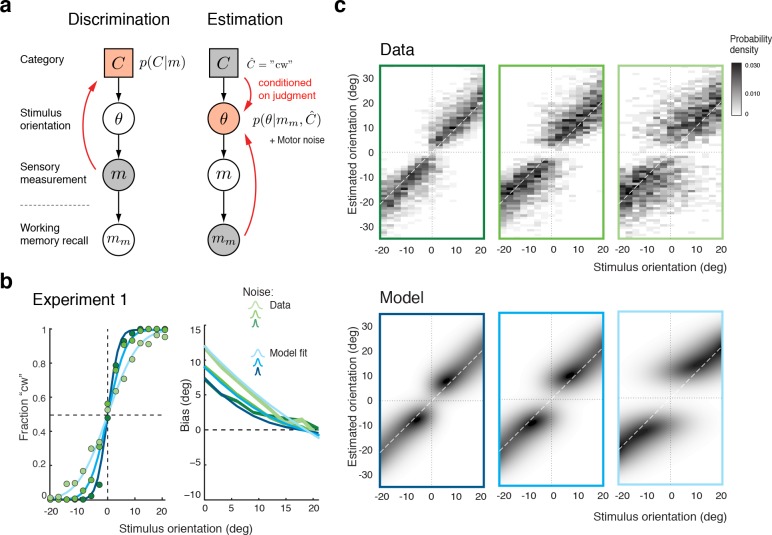
Figure 3. The self-consistent Bayesian observer model.
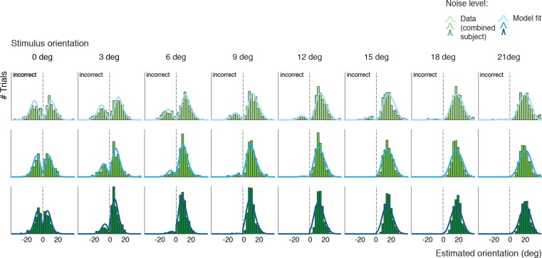
(a) Directed graph representing the generative hierarchical model: Sensory measurement is a noisy sample of stimulus orientation . Every belongs to one of two categories . Given an observed , the self-consistent model first performs inference over (discrimination task), and then infers the value of conditioned on the preceding discrimination judgment (e.g., ) (estimation task). Inference for the estimation task is assumed to be based on a noisy memory recall of the sensory measurement . Conditioning on the categorical choice sets the posterior to zero for all values of that do not agree with the choice. This shifts the posterior probability mass away from the discrimination boundary and results in the repulsive post-decision biases for any loss function that more strongly penalizes large errors than small ones. Because subjects were instructed to provide estimates as accurate as possible we assumed a loss function that minimizes mean squared-error ( loss). (b) We jointly fit the observer model to all discrimination-estimation data pairs of the combined data across all subjects in Experiment 1 (combined subject). (c) The model not only predicts the mean estimation bias (as shown in (b)) but also the entire distributions of estimates, including those trials where discrimination judgments were incorrect. Data and model show the characteristic bimodal pattern for orientation estimates. Each column corresponds to one of the three stimulus noise conditions.


