

Abstract
Researchers continue to be interested in efficient, accurate methods of estimating coefficients of covariates in mixture modeling. Including covariates related to the latent class analysis not only may improve the ability of the mixture model to clearly differentiate between subjects but also makes interpretation of latent group membership more meaningful. Very few studies have been conducted that compare the performance of various approaches to estimating covariate effects in mixture modeling, and fewer yet have considered more complicated models such as growth mixture models where the latent class variable is more difficult to identify. A Monte Carlo simulation was conducted to investigate the performance of four estimation approaches: (1) the conventional three-step approach, (2) the one-step maximum likelihood (ML) approach, (3) the pseudo class (PC) approach, and (4) the three-step ML approach in terms of their ability to recover covariate effects in the logistic regression class membership model within a growth mixture modeling framework. Results showed that when class separation was large, the one-step ML approach and the three-step ML approach displayed much less biased covariate effect estimates than either the conventional three-step approach or the PC approach. When class separation was poor, estimation of the relation between the dichotomous covariate and latent class variable was severely affected when the new three-step ML approach was used.
Keywords: latent growth modeling, growth mixture modeling, latent class analysis, covariate effect
Growth mixture modeling (GMM; B. O. Muthén, 2001, 2004; B. O. Muthén & Muthén, 2000; B. O. Muthén & Shedden, 1999) continues to be a popular platform for practitioners in the social and behavioral sciences to examine population heterogeneity in growth characteristics of individuals’ longitudinal profiles, and the number of applications in recent years has increased appreciably (see, e.g., Colder, Campbell, Ruel, Richardson, & Flay, 2002; Colder et al., 2001; Ellickson, Martino, & Collins, 2004; Heybroek, 2011; Huang, Murphy, & Hser, 2012). The number of methodological studies investigating growth mixture models has increased, and investigations have been conducted to ascertain information on the optimal number of latent classes, estimation performance under model misspecification, and accuracy of the classification of individuals into groups (see, e.g., Liu, 2012; B. O. Muthén, 2004; Nylund, Asparouhov, & Muthén, 2007; Petras & Masyn, 2010; Tofighi & Enders, 2008). More recently, the methodological issue of systemic bias of covariate effects in mixture modeling has surfaced (Bolck, Croon, & Hagenaars, 2004; Nylund-Gibson & Masyn, 2009; Vermunt, 2010). Although a number of interesting modeling solutions have been recommended including the pseudo-draw approach (Bandeen-Roche, Miglioretti, Zeger, & Rathouz, 1997; Clark & Muthén, 2009, Wang, Brown, & Bandeen-Roche, 2005), the BCH method (Bolck et al., 2004; Croon, 2002), and a modified three-step approach in which classification error probabilities are taken into account (Asparouhov & Muthén, 2013; Vermunt, 2010), there has not been to date a systematic exploration of these potential solutions in the context of GMM.
In this article, the notation of GMM mixture models used in discerning growth trajectories for unobserved groups is reviewed first followed by a brief review of model-based and post hoc methods of estimating covariate effects. We follow this exposition with a Monte Carlo simulation examining the performance of these methods under scenarios suggested from the literature and based on our own work. The results from the simulation are subsequently discussed and framed as recommendations to practitioners concluding with some thoughts on future methodological directions that could build on this study.
Incorporating Covariates in Growth Mixture Modeling
Growth Mixture Models
Conceptually, GMM is a combination of what is typically referred to as latent growth modeling (Bollen & Curran, 2006; McArdle, 1988; Meredith & Tisak, 1990) and latent class analysis (Collins & Lanza, 2010; Lazarsfeld & Henry, 1968; McCutcheon, 1987). These unknown latent classes arise when genuinely distinct clusters of change exist, but are embedded within individuals’ growth patterns. Latent classes are identified by allowing structured heterogeneity in the random effects and residual error populations through incorporating mixtures of normal distributions although this particular specification can be relaxed (see, e.g., B. O. Muthén & Asparouhov, 2009). These distributions are used to classify longitudinal profiles into different mixture components. In one of its simplest forms, an unconditional linear growth mixture model for repeated measurements of a continuous dependent variable can be presented by using a general structural equation modeling notation:
where is a vector of repeated measures for individual i, is a vector of individual-specific growth factors (i.e., intercept and slope), and is a matrix of factor loadings. The vector of time-specific errors, captures the deviations from the data to the fitted model for each individual within a class (Bauer, 2007). Within each class, the error terms are assumed to be normally distributed:
with mean vector of 0. The covariance matrix can take on a number of different structures depending on the situation (see, e.g., Harring & Blozis, 2014), but is often relegated to a simple structure like a mutually independent homogeneous error structure once between-subject variability has been accounted for in the model. At the population level, given class k, individual-specific growth factors are formulated initially as the sum of fixed and random effects,
and are assumed to be multivariate normally distributed
where class-specific fixed effects, capture the differences in the growth factor means of the latent classes. The growth factor variances and covariances are also class specific and are contained in covariance matrix, The random effects, and the residuals, are uncorrelated (i.e., cov() = 0).
Inclusion of Covariates in GMM
Once class enumeration has been completed with an appropriately specified unconditional growth mixture model, the focus of the analysis usually shifts to investigating the effects of covariates on the system. As Figure 1 shows, covariates can enter the general growth mixture model in three different ways. First, covariates can be included in the growth model as antecedents or predictors of individual differences in the underlying change process (Petras & Masyn, 2010). These relations are depicted by the dashed lines coming from time-invariant covariate(s) x and pointing to the latent linear growth factors, intercept () and slope (). Covariates can also enter the entire GMM system through a multinomial logistic regression model that relates individual attributes and characteristics to latent class membership. In Figure 1, this is a single-headed arrow from x to categorical latent class variable, C. Last, covariates can enter the growth mixture model through the appropriate modeling of some distal outcome or sequelae of change, Z, and its direct effect is denoted via the single-headed arrow from x to Z. Since the new three-step method, as it is implemented in Mplus 7.3 (L. K. Muthén & Muthén, 2014), can only treat the latent class membership model or the distal outcome model, but not both simultaneously, in the current study, we only examine the impact of different methods of estimating the growth mixture model in the presence of covariates that predict latent class membership.
Figure 1.
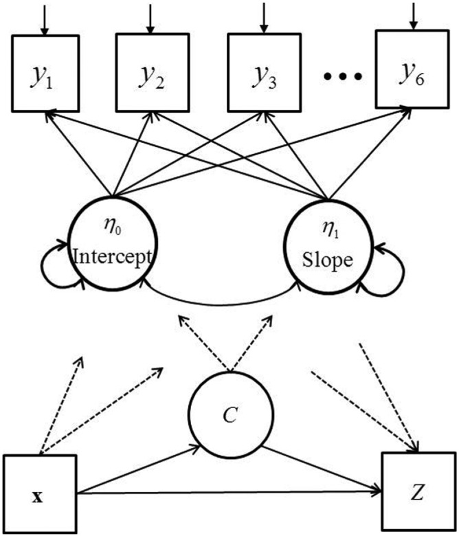
Path diagram for a general linear growth mixture model with time-invariant covariates, x, and distal outcome, Z.
Approaches to Estimating Covariate Effects in GMMs
In GMM, it is universally accepted that incorporating covariate information in an analysis is beneficial in terms of more accurate parameter estimates and refinement of the latent classes themselves (see, e.g., Huang, Brecht, Hara, & Hser, 2010; Li & Hser, 2011), yet there has been disagreement regarding the timing of when covariates should be included. According to Bauer and Curran (2003), the common practice of using GMM without covariates for class enumeration has been questioned in the methodological literature. Obviously this practice implicitly assumes that fitting growth mixture models without covariates would recover the correct number of classes whether or not the covariates affect class membership or growth factors in the population. However, this assumption may not hold universally (B. O. Muthén, 2004). According to B. O. Muthén (2004), auxiliary information in terms of predictors or covariates of the latent factors and latent group membership, as well as distal static outcomes of trajectory group membership (Lubke & Muthén, 2007; Petras & Masyn, 2010), can be efficiently included in a GMM analysis to obtain more accurate parameter estimates and latent class assignment. Previous research has suggested that covariates of latent group membership be included when deciding on the number of latent classes (Lubke & Muthén, 2007; B. O. Muthén, 2003, 2004), while others have advocated their inclusion only after the class enumeration process (Bauer, 2007; Nylund-Gibson & Masyn, 2009; Petras & Masyn, 2010). This distinction has played an important role in the development of new analytic techniques in handling covariates.
Various approaches have been proposed to estimate growth mixture models with covariates. A conventional step-by-step approach to including covariates in a latent class analysis may involve the following steps: First, the unconditional latent class model is fitted based only on latent class indicators to determine the number of distinct latent groups. In terms of GMM, the latent class indicators are used to determine the number of distinct trajectory groups (D’Unger, Land, & McCall, 2002; Feng, Shaw, & Silk, 2008; Fergusson & Horwood, 2002; Jo, Wang, & Lalongo, 2010; McDermott & Nagin, 2001; Nagin, Farrington, & Moffitt, 1995; Nagin & Land, 1993). Then, in the second step, predicted posterior class membership probabilities are calculated and class membership is assigned to each individual based on their highest posterior class membership probabilities. Finally, the relation between the assigned latent class membership and subject-specific background characteristics is investigated using either mean comparison tests or multinomial logistic regression models (Clark & Muthén, 2009). One issue that arises with this method is that class membership is treated as an exact, observed variable without taking into account the error associated with estimating these probabilities (Clark & Muthén, 2009), which will lead to underestimated associations between covariates and class membership (Bolck et al., 2004).
To correct the conventional three-step approach, Bolck et al. (2004) and Croon (2002) developed the BCH method where class assignments are summarized in a multidimensional frequency table that is reweighted via a matrix multiplication by the inverse of the matrix of classification errors, and then the reweighted data are analyzed using a standard logistic regression. However, one major limitation with this approach is that only categorical covariates can be included, and the severely downward biased standard errors are found for the logistic regression coefficients by using this method. Vermunt (2010) later proposed a modified BCH procedure so that continuous predictors or distal outcomes can be used. This modified BCH approach is preferable because it removes the downward bias in the standard errors by using the linearization variance estimator (Vermunt, 2010).
On the other hand, rather than treating information on the individual as an outcome in post hoc comparisons as is done in the conventional approach, a one-step maximum likelihood (ML) approach (see, e.g., Clogg, 1981; Dayton & Macready, 1988; Haberman, 1979; Hagenaars, 1990, 1993; Huang et al., 2010; B. O. Muthén, 2004; Nagin, 2005; Roeder, Lynch, & Nagin, 1999; Van der Heijden, Dessens, & Böckenholt, 1996; Vermunt, 1997) was recommended that incorporates the covariates as part of a single model. The one-step approach takes into account the error associated with probability estimates by allowing individuals to be fractional members of all classes (Clark & Muthén, 2009). However, one major issue with this approach may be that the latent classes formed from the joint model may differ in meaning from the latent classes obtained using the indicator variables alone and thus may potentially change their substantive interpretation; on the other hand, simultaneously building the classification model and the prediction model may not fit with the logic of most applied researchers, who often work sequentially from first building the classification model then adding covariates at a secondary stage of the analysis (Vermunt, 2010).
To independently evaluate the relation between the latent class variable and the covariates without using assigned class membership, pseudo class (PC) draws (Asparouhov & Muthén, 2006; Bandeen-Roche et al., 1997; Clark & Muthén, 2009; Wang et al., 2005) was proposed. With the PC method, for the latent class analysis, multiple random samples are drawn from a multinomial distribution of posterior probabilities (for each individual) being in each class so that each individual is given a chance to fall into neighboring classes (Clark & Muthén, 2009). Finally, the class-specific information associated with the covariate(s) is obtained using the multiple imputation techniques developed by Rubin (1987).
The three-step ML approach has recently been proposed by Vermunt (2010). In this fairly recent approach, the unconditional growth model would first be estimated, which is exactly the same as the initial step in the conventional three-step approach. A most likely class variable is subsequently defined using the highest posterior probability from the latent class posterior distribution derived from the unconditional growth mixture analysis. In the third step, the most likely class variable is used as latent class indicator variable with classification error probability taken into account. During this final stage of model estimation, covariates or relevant predictors are introduced with the unconditional GMM kept fixed. Therefore, the big difference between the new three-step ML approach and the conventional three-step approach is in the third step where the most likely class membership variable is treated as an imperfect measurement of latent class membership analysis in the new approach but not in the conventional approach. Asparouhov and Muthén (2013) discussed in detail the procedures of calculating classification error probability. A matrix of average class membership probabilities is established first, where is the most likely class variable with s rows and is the true latent class variable with k columns. Within each of the most likely latent classes, the average probability of membership for the most likely latent class as well as the remaining, “less likely” classes for the matrix are computed. A matrix of corrected average probabilities of class membership is subsequently derived using
where s and k stand for, respectively, the sth row (s = 1 through s) and kth column (k = 1 through k) of the matrix, and represents the sample size for the most likely class on the sth row. In the third step, the most likely class variable is used as a latent class indicator variable with uncertainty rates prefixed at the probabilities (Asparouhov & Muthén, 2013). That is, the most likely latent class variable is specified as a nominal indicator of the latent class variable with logits, where S is the last class. These logarithmic ratios would enter directly into the secondary statistical analysis as indicators of measurement error in assigning cases to classes.
A Brief Overview of Past Methodological Studies
Studies have been conducted recently to compare the performance of some of these approaches to estimating the effects of covariates in mixture modeling. The main purposes of these studies were to see how efficient and reliable these methods were in terms of estimating the association between the latent class variable and auxiliary information under different conditions. For example, using simulated and real data, Clark and Muthén (2009) explored how different regression methods of relating latent class analysis results to covariates affected estimation accuracy of the covariate effects. Results showed that the one-step approach performed the best in terms of recovering the true covariate effect. The PC method worked well when class separation was large. When class separation was not large, like the conventional regression methods, the PC method underestimated the standard errors, which was problematic because an effect may be identified as significant, when in fact, it may not have been (Clark & Muthén, 2009). In another study, Vermunt (2010) compared the conventional three-step procedure, the one-step approach, the modified BCH approach, and his proposed three-step ML approach with respect to bias in the estimates of the covariate effects and bias in the standard error estimates when covariates were included in a latent class analytic context. Results showed that the conventional three-step approach performed poorly in the sense that its parameter estimates were severely biased downward. The modified BCH method and the three-step ML method both demonstrated acceptable parameter recovery and unbiased standard errors, except when the classes were very poorly separated. It was also found that the three-step ML method was much more efficient than the BCH method in terms of the standard errors of the parameter estimates, and it was nearly as efficient as the one-step estimation approach. In a very recent unpublished study by Asparouhov and Muthén (2013), the relation between a latent class variable and predictor variable in mixture modeling was examined using different approaches under a small number of design factors. Results showed that the new three-step ML approach uniformly outperformed the PC approach for analyzing the relation between a latent class variable and a covariate independent of the latent class model estimation approach. In addition, in the case when class separation was substantial, the three-step ML approach had the same efficiency as the one-step approach in terms of bias, mean squared error, and confidence interval coverage of the parameter estimates. In another recent study, Bakk, Tekle, and Vermunt (2013) used both simulated and real data to investigate the association between distal outcomes and latent class variable using different methodological approaches. The results showed that the conventional three-step approach led to severely biased parameter estimates compared with other methods like the three-step ML method. However, when class separation was low, the three-step ML method underestimated the parameter estimates and their corresponding standard errors.
One limitation with these studies is that very simple latent class models for discrete responses were used. Although Asparouhov and Muthén (2013) also included more complicated models such as a growth mixture model to evaluate how well different estimation approaches performed, like most previous studies, their study included only one covariate and had a very limited number of manipulated factors and levels within those factors. Vermunt (2010) included three predictor variables in his simulation study; however, all the predictor variables were categorical and uncorrelated—a seemingly unrealistic scenario. It is quite possible that in real data analytic settings many covariates of different types would be considered simultaneously. Bakk et al. (2013) included only distal outcome variables in their latent class analyses. Another limitation found in Asparouhov and Muthén’s (2013) study with respect to GMM is that although three different types of direct effects from the auxiliary information on the growth factors were manipulated, the impact of the covariates with various effect sizes on the new three-step ML approach was not investigated.
Method
A Monte Carlo simulation is conducted to assess the performance of four approaches to estimating the association between covariate(s) and the latent class variable under the GMM framework: (1) the conventional three-step approach, (2) the one-step ML approach, (3) the PC approach, and (4) the new three-step ML approach. Since the current study uses Mplus Version 7.11, which does not implement the modified BCH approach, the modified BCH approach is not included in the research.
Experimental Design
Four fixed factors are considered. The number of repeated measures is fixed at six assuming all individual growth trajectories in each subpopulation start and end at the same point. It is often seen in both simulation studies and substantive research of growth mixture models that the number of measurement occasions is three or more (see, e.g., Brown, 2003; Jung & Wickrama, 2008; Masyn & Brown, 2001), and it has been recommended that a minimum of three time points be used to specify a linear model (Willett, Singer, & Martin, 1998). Simon, Ercikan, and Rousseau (2012) suggested a minimum of four repeated measures to achieve more power in growth modeling. On the other hand, considering the potential issues regarding convergence or power, at least five indicators have been recommended (B. O. Muthén & Curran, 1997). Therefore, the choice of six time points seemed reasonable. As per the number of latent classes, a two-latent class model was chosen so as to keep the scope of the study manageable. In terms of distributions of two covariates used in the study, proportions for the dichotomous covariate, were fixed at 30:70 and the continuous covariate, was drawn from a standardized normal distribution with a mean of 0 and variance of 1. Only time-invariant covariates were considered in the analyses.
Some simplifying assumptions were made in order to keep the scope of the study feasible considering the complexity of the model. Measured outcome variables, for example, were specified as continuous coming from a multivariate normal distribution and that individual growth trajectories were assumed to be linear. It was also presumed that residual variances among measured indicator variables were invariant over the classes (i.e., for all k) and were homoscedastic and uncorrelated (i.e., ), and that growth factor covariance matrices were unstructured and invariant across latent trajectory classes (i.e., for all k). Since model complexity is one factor that makes model convergence a potential issue, it has been recommended that residual variances among indicator variables as well as growth factor variances and covariances be constrained equal across classes to ensure the absence of singularities and to ensure the existence of a global solution (Hipp & Bauer, 2006; Liu, Hancock, & Harring, 2011). It should be added that parameters for growth factor covariance matrices and residual variance used were defined as
It has been advocated in several simulation studies on latent growth models and GMMs that, in practice, the ratio of the intercept variance to the slope variance is approximately 5:1 (see, e.g., Depaoli, 2013; Liu, 2012). In line with the consistency of this recommendation from the literature, the diagonal values in were chosen in this ratio with the covariance set so that the correlation between the random effects was approximately 0.50.
Four manipulated factors were considered in the current study (see Table 1). Abbreviations of these factors were included in the parentheses to make later presentation of the results concise. The level(s) of these factors were selected based on a thorough review of relevant studies. Four levels of the factor sample size were considered: 500, 1,000, 5,000, and 10,000. A review of the literature has shown various sample sizes ranging from 25 to 10,000. However, for latent class analyses, a sample size of 500 was considered small especially when classes were not well-separated (Vermunt, 2010). A sample size of 1,000 was selected because it was a typical sample size level used in methodological GMM studies (see, e.g., Brown, 2003; Clark & Muthén, 2009; Kohli, 2011; Nylund et al., 2007; Tolvanen, 2008; Vermunt, 2010). The choice of a sample size of 5,000 was consistent with one of the manipulated conditions for growth mixture models by Asparouhov and Muthén (2013) whose work has been extended into this particular study, and a very large sample size of 10,000 (see, e.g., Vermunt, 2010) was added to avoid sampling fluctuation as well as to increase the convergence rate. Results from previous studies (see, e.g., Nylund et al., 2007; Tofighi & Enders, 2008) have indicated that the mixing proportion played an important role in growth mixture analyses. The current study manipulates mixing proportion conditions at two levels: 30:70 and 50:50. More extreme levels such as 10:90 have led to severe convergence issues in past studies (e.g., Tolvanen, 2008) and thus were not investigated in this study.
Table 1.
Manipulated Factors.
| Factor | Levels |
|---|---|
| Sample size (N) | Level 1: 500 |
| Level 2: 1,000 | |
| Level 3: 5,000 | |
| Level 4: 10,000 | |
| Mixing proportions (MP) | Level 1: 30%:70% |
| Level 2: 50%:50% | |
| Degrees of class separation (CS), measured by Mahalanobis distance (MD) | Level 1: MD = 1.0 |
| Level 2: MD = 2.0 | |
| Level 3: MD = 3.5 | |
| Covariate effect (CE), measured by odds ratio (OR) | Level 1: OR for = 1.5, OR for = 1.5 |
| Level 2: OR for = 9.0, OR for = 9.0 | |
| Level 3: OR for = 1.5, OR for = 9.0 | |
| Level 4: OR for = 9.0, OR for = 1.5 |
Perhaps the most important condition to be manipulated is class separation. In the current study, class separation is measured in terms of the multivariate Mahalanobis distance (MD; Mahalanobis, 1936) between two latent classes of random effects and was manipulated by varying the latent growth factors (e.g., growth trajectory intercept and slope). Previous studies indicated that estimation accuracy in GMM had been largely affected by how well subpopulations were separated (see, e.g., Everitt, 1981; Lubke & Muthén, 2007; Tofighi & Enders, 2008). Class separation can occur at the latent level or the measured variable level (see, e.g., Tolvanen, 2008). This study focuses exclusively on class separation at the latent level for the growth parameters. MD between two latent classes is defined as follows:
where and are the growth factor means for the first and second latent classes, respectively (McLachlan & Peel, 2000), and represents the inverse of the common covariance matrix of individuals’ growth parameters. Referring to previous studies and also based on exploratory analyses in a pilot study conducted at the onset, the current research sets MDs at 1.0, 2.0, and 3.5 to reflect small, large, and very large growth trajectory separation conditions, respectively (see, e.g., Depaoli, 2013; Everitt, 1981; Lubke & Muthén, 2005; Lubke & Neale, 2006; Tolvanen, 2008; Tueller & Lubke, 2010).
In terms of covariate effects, the strength of the association between the two covariates and latent class membership was manipulated using the odds ratio (OR). Two levels of OR, 1.5 and 9.0, were set indicating small and large effects, respectively (see, e.g., Cohen, 1988). Therefore, four sets of covariate effects for and were manipulated, which are, 1.5 for both and at CE = 1, 9.0 for both and at CE = 2, 1.5 for and 9.0 for at CE = 3, and 9.0 for and 1.5 for at CE = 4.
The data generation model takes the form of the logistic regression function to model the relation between covariates and the latent classes. Two covariates are generated as predictors of an individual being in a latent class through the multinomial logistic regression equation given as
where is a dichotomous covariate (e.g., gender) defined with values of 0 or 1, and is a continuous covariate (e.g., aptitude) having been generated from a standardized normal distribution with a mean of 0 and variance of 1. The regression coefficients, and represent the effect of covariates on the log odds of membership in class k relative to class K, and is the logistic regression intercept for class k relative to class K. For simplicity, interaction between the two covariates was not considered in this study. For purposes of model identification, latent class 2 is considered the reference class, and then coefficients, , , and were all fixed to 0. It should be noted that the predictors, and , are generated such that the strength of the correlation between them is weak to moderate and positive, 1 Inducing the correlation between categorical and continuous variables is to mimic the real-life situation where most of the variables are correlated and independent relations between variables seldom exists.
In summary, four levels of sample size, three levels of class separation, two levels of mixing proportion, and four sets of covariate effects are used in the experimental design, which results in 4 × 3 × 2 × 4 = 96 cells. Since four estimation approaches are examined under each of these cells, the total number of conditions is 96 × 4 = 384.
Altogether, 500 replications that achieve convergence to the global solution across all approaches in each cell of the design are required. In methodological studies focused on GMM, the minimum number of replications has been found to be 100 (see, e.g., Asparouhov & Muthén, 2013). Many studies have used 500 replications (see, e.g., Bauer & Curran, 2003; Brown, 2003; Nylund et al., 2007), which has also been an advocated number of replications in a recent book chapter by Bandalos and Leite (2013) to ensure an accurate portrayal of the precision in the estimates.
Data were generated and analyzed using Mplus Version 7.11 (Muthén & Muthén, 2014). While different estimation algorithms have been developed for mixture analyses, the current study limits the discussion to ML estimation implemented via the EM algorithm, which remains by far the most popular estimation method used in GMM analyses and is accessible through commercial software.
Criteria for Evaluating Approaches to Estimation Covariate Effects
The outcome measures to be compared in this simulation study include: (1) percent relative bias in the estimates of the covariate effects, (2) variance of the covariate effect estimates, and (3) standard error efficacy (bias) of the covariate effect estimates.
Relative bias is used to remove the scale of the parameter in its calculation putting the values on equal footing. A percent relative bias is obtained by dividing the bias of a parameter estimate (i.e., estimate of a covariate effect) by the population parameter value, which is expressed as
where is the expected covariate estimates computed from the replicate data sets within each cell of the design, is the true covariate effects, and is the bias of parameter estimate.
Variance of covariate effect estimates within each cell is also compared to examine the variability of parameter estimates using its empirical sampling distribution, and is calculated as
Standard error efficacy of the covariate effect estimates is used as another criterion for estimation approach comparison, which can be obtained using
where is the square root of the mean variance of derived from the 500 replications, and , which is the corrected sample standard deviation of 500 parameter estimates in a given cell. If the estimated standard errors computed based on an approach are accurate, the ratio of to should be close to 1 (Lee, 2007; Lee, Song, & Poon, 2004). A standard error efficacy value greater than 1 indicates that the standard errors are overestimated, implying increase of committing Type II errors by the model, whereas a value less than 1 indicates that the standard errors are underestimated by the model (chance of committing Type I errors).
Preliminary GMM Analyses
Using the collated data for the three evaluation criteria as dependent variables, three separate repeated measures ANOVAs were conducted to determine the statistical significance of the effects of the different levels of the manipulated factors in various covariate estimation approach conditions. In the ANOVA analyses, all conditions were treated as the fixed effects. In summary, four main effects (i.e., sample size, degrees of class separation, mixing proportion, and covariate effects) and their interaction terms, up to three-way interaction, were included in the analysis. In addition to test the statistical significance, in order to determine the practical significance of the effect, an effect size index, eta-square (), which is defined as was also assessed. An of 0.06 indicates a medium sized effect (see, e.g., Cohen, 1988) and was used as a cutoff for practical significance with smaller values denoting impractical significance. Using the results from the factorial ANOVAs guided which findings to focus on when reporting the results of the simulation studies.
Results
Performance of the four approaches was investigated using results from 500 replications that achieved convergence to the global solution. It should be mentioned that convergence issues are regularly found in mixture model studies. Since the current study only examines the parameter recovery in converged cases, low convergence rates will undermine the evaluation of parameter recovery and subsequent factorial analysis of variance results. Therefore, new data sets were generated and estimated until 500 replications achieved convergence to the global solution across all approaches under investigation. Three separate repeated-measures ANOVAs were conducted in SPSS (version 18.0), with percent relative bias, parameter estimate variance, and standard error efficacy used as dependent variables, to determine the statistical significance of the effects of the different levels of the manipulated factors in various covariate estimation approaches. The main effects and up to the three-way interaction effects were reported in the tables only if they were identified to be both statistically significant (p value ≤.05) and had an effect size of (see, e.g., Cohen, 1988; Kohli, 2011). The Huynh-Feldt correction was used to adjust the degrees of freedom when the sphericity assumption was not met.
Percent Relative Bias
Descriptive statistics showed that generally for all levels of covariate effect the magnitude of percent relative bias related to both covariates tended to be closer to 0 for all approaches under each combined condition of sample size and mixing proportion when class separation increased. For all levels of covariate effects, the PC approach and the conventional three-step approach tended to underestimate the covariate effects. Generally at all levels of covariate effects, relative bias values were much closer to 0 for the one-step ML approach and the three-step ML approach than for the PC approach or the conventional three-step approach at any combined level of condition, suggesting the former two approaches produced less biased parameter estimates.
A repeated-measures ANOVA was conducted where percent relative bias was modeled as a function of the manipulated simulation conditions. To make presentation of the results simple, symbols were used for the estimation approaches: A for approach to covariate effects estimation, A1 for the conventional three-step approach, A2 for the one-step ML approach, A3 for the PC approach, and A4 for the three-step ML approach. Table 2 shows that estimation approach had a significant main effect on percent relative bias of covariate effect estimates related to both () and (). Sample size, class separation, and covariate effect had significant main between-replications effects on percent relative bias of covariate effect estimates for An effect size of for the main effect of covariate effect suggested that estimation accuracy for the dichotomous covariate effect was greatly influenced by the levels of covariate effect manipulated. Significant two-way interaction effects for were identified for A × CS (), N × CE (), and CS × CE (). Significant two-way interaction effect from A × CS was also found for (). The only significant three-way interaction effect was found for A × CS × CE () for A detailed explanation of the interaction effects (related to approaches to covariate effects estimation) rather than the main effects was followed for a more complete picture. In addition, if a two-way interaction varies across the levels of a third variable, the three-way interaction instead of the two-way interaction were discussed. Therefore, only the influence of A × CS on and the influence of A × CS × CE on were discussed.
Table 2.
ANOVA Results of Manipulated Factors on the Percent Relative Bias.
| Source |
|
|
||||
|---|---|---|---|---|---|---|
| F value | p value | F value | p value | |||
| Within-replications effectsa | ||||||
| A | 701.257 | <.001 | 0.46 | 911.395 | <.001 | 0.64 |
| A × CS | 188.106 | <.001 | 0.25 | 141.512 | <.001 | 0.20 |
| A × CS × CE | 24.828 | <.001 | 0.10 | |||
| Between-replications effects | ||||||
| N | 28.612 | <.001 | 0.06 | |||
| CS | 43.073 | <.001 | 0.06 | |||
| CE | 123.824 | <.001 | 0.27 | |||
| N × CE | 15.572 | .003 | 0.10 | |||
| CS × CE | 63.233 | <.001 | 0.28 | |||
Note. A = approach to covariate effects estimation; CS = degree of class separation; CE = covariate effect; N = sample size.
The Huynh-Feldt correction was used to adjust the degrees of freedom if necessary.
Graphics were created to visually understand the identified significant interaction effects to be discussed. Figure 2(a) showed the two-way interaction effect of A × CS on percent relative bias related to the continuous variable It was observed that when class separation was larger, percent relative bias was closer to the desired value of 0 for the conventional three-step approach and the PC approach, and that percent relative bias values were close to 0 across all levels of class separation for both the one-step ML approach and the three-step ML approach, suggesting that the one-step ML approach and the three-step ML approach led to less biased parameter estimates than either the conventional three-step approach or the PC approach at all levels of class separation when the covariate was continuous. In terms of the three-way interaction effect of A × CE × CS related to the dichotomous covariate , four two-way interaction effects of A × CS were graphed for each level of covariate effect (see Figure 2a-e). Similar to what was observed in Figure 2(a), percent relative bias was closer to 0 for the conventional three-step approach and the PC approach when class separation increased at all levels of covariate effect, and percent relative bias values for these two approaches were very close to 0 at MD = 3.5. It was also observed, however, that percent relative bias related to was affected by the size of covariate effect when the one-step ML approach or the three-step ML approach was used. Specifically, at CE = 2 (see Figure 2c) and CE = 4 (see Figure 2e) where covariate effect related to was big, percent relative bias values were very close to 0 for both the one-step ML approach and the three-step ML approach across all levels of class separation; however, percent relative bias values departed further away from the desired value of 0 for these two approaches at CE = 1 (see Figure 2b) and CE = 3 (see Figure 2d) where covariate effect related to was small at MD = 1.0, especially for the three-step ML approach, suggesting that parameter estimate related to the dichotomous covariate was very sensitive to poor class separation for the one-step ML approach and the three-step approach when the association between the dichotomous covariate and the class membership was small. It was also noticed in Figures 2(a) to (e) that percent relative bias values are very close between the conventional three-step approach and the PC approach.
Figure 2.

Interaction effects on percent relative bias and variance of covariate effect estimates.
Note. A = approach to covariate effects estimation; CS = degree of class separation; CE = covariate effect.
Variance of Covariate Effect Estimates
Compared to bias that indicates how close on average the estimates are to the true parameter, variance of covariate effect estimates suggests how much the parameter estimates change across the sample replications. That is, variance of parameter estimates is calculated using the mean of the estimates for each cell instead of the true value of the parameter in measuring parameter estimate variability. As expected, variances of covariate effect estimates for the conventional three-step approach and the PC approach were generally smaller than those for the one-step ML approach or the three-step ML approach at each combined level of sample size, mixing proportion, class separation, and covariate effect. More variability was noticed for the one-step ML approach and the three-step ML approach than for the other two approaches for all levels of covariate effects. The smaller variance of the PC approach and the conventional three-step approach suggests that these two approaches consistently underestimate the parameters under investigation, which explains why the relative bias from these two approaches is high. It should be mentioned, however, that the largest variance was found at MD = 1.0 for all four approaches investigated, meaning that when class separation was poor, covariate effect estimation had more variability regardless of which approach was used.
Variance of covariate effect estimates was modeled also as a function of the manipulated simulation conditions. The ANOVA results in Table 3 showed that approach, sample size, mixing proportion and class separation had significant main effects on variance of covariate effect estimates related to Class separation was also identified as a significant main effect related to (). Significant two-way interaction effect of A × CS was found related to both () and (). Only one three-way interaction effect (A × CS × CE) related to was found significant with an effect size of
Table 3.
ANOVA Results of Manipulated Factors on the Variance of Covariate Effects Estimates.
| Source |
|
|
||||
|---|---|---|---|---|---|---|
| F value | p value | F value | p value | |||
| Within-replications effectsa | ||||||
| A | 157.593 | <.000 | 0.28 | |||
| A × CS | 108.551 | <.000 | 0.38 | 3.137 | .010 | 0.08 |
| A × CS × CE | 1.981 | .028 | 0.15 | |||
| Between-replications effects | ||||||
| CS | 154.636 | <.000 | 0.57 | 4.748 | .022 | 0.12 |
| N | 10.619 | <.000 | 0.06 | |||
| MP | 33.534 | <.000 | 0.06 | |||
| N × CS | 5.247 | .003 | 0.06 | |||
| MP × CS | 15.358 | <.000 | 0.06 | |||
Note. A = approach to covariate effects estimation; CS = degree of class separation; CE = covariate effect; N = sample size; MP = mixing proportions.
The Huynh-Feldt correction was used to adjust the degrees of freedom if necessary.
Effect of the two-way interaction of A × CS on the variance of covariate effect estimates related to and are displayed in Figure 2(f) and (g), respectively, where a similar pattern was observed. As might be expected, for both and , variance values were always close to 0 for all estimation approaches at MD = 3.5. Variance values were always close to 0 for all class separation levels when the conventional three-step approach and the PC approach were used, suggesting parameter estimates did not vary much across the sample replications at any class separation level when these two approaches were used. Variances of covariate effect estimates for both and were close to 0 at MD = 2.0 and MD = 3.5 when the one-step ML approach or the three-step ML approach was use. At MD = 1.0, though, both the one-step ML approach and the three-step ML approach showed large variances, suggesting that these two approaches were sensitive to low class separation in terms of variability of covariate effect estimates. The three-way interaction effect of A × CS × CE on the variance of parameter estimates related to showed exactly the same patterns across all levels of covariate effect and thus was not discussed in detail.
Standard Error Efficacy of the Covariate Effect Estimates
Descriptive statistics in standard error efficacy for the covariate effect estimates suggested that for all combined levels of sample size, mixing proportion, and covariate effect, standard error efficacy values related to both and were closest to 1 for all estimation approaches when class separation was at the highest considered level of MD = 3.5. The PC approach attained efficacy values greater than 1 across all levels of sample size, mixing proportion and class separation, suggesting higher probability of committing Type II errors.
Results of the repeated-measures ANOVA for the standard error efficacy of the covariate effect estimates are displayed in Table 4. Estimation approach and covariate effect both had significant main effect for and In terms of interaction effects, A × CS, A × CE, and CE × CS all had significant effects on standard error efficacy for both and . Significant three-way interaction effect on standard error efficacy was found for A × CE × CS for both and , and for N × CE × CS related only to Because the purpose of the current research is to investigate the performance of different approaches in terms of their ability to recover covariate effect, the three-way interaction effects of A × CE × CS related to and were the main focus of the discussion.
Table 4.
ANOVA Results of Manipulated Factors on the Standard Error Efficacy.
| Source |
|
|
||||
|---|---|---|---|---|---|---|
| F value | p value | F value | p value | |||
| Within-replications effectsa | ||||||
| A | 118.967 | .000 | 0.37 | 113.842 | .000 | 0.40 |
| A × CS | 35.041 | .000 | 0.22 | 21.983 | .000 | 0.16 |
| A × CE | 6.639 | .000 | 0.06 | 7.147 | .000 | 0.08 |
| A × CE × CS | 4.081 | .000 | 0.08 | 5.697 | .000 | 0.12 |
| Between-replications effects | ||||||
| CS | 32.998 | .000 | 0.26 | |||
| CE | 18.732 | .000 | 0.22 | 19.276 | .000 | 0.23 |
| N × CE | 3.057 | .021 | 0.11 | |||
| N × CS | 3.343 | .022 | 0.08 | |||
| CE × CS | 3.743 | .014 | 0.09 | 10.250 | .000 | 0.24 |
| N × CE × CS | 2.533 | .028 | 0.18 | |||
Note. A = approach to covariate effects estimation; CS = degree of class separation; CE = covariate effect; N = sample size.
The Huynh-Feldt correction was used to adjust the degrees of freedom if necessary.
Graphics for the three-way interaction effects of A × CE × CS on standard error efficacy related to and are presented in Figures 3(a) to (h). It was observed that for both and across all covariate effect levels, all approaches investigated led to standard error efficacy values close to 1 when class separation was as large as MD = 3.5. At MD = 2.0, the PC approach showed larger distance away from the desired efficacy value of 1 compared with the other three approaches, suggesting that the PC approach requires sufficiently large class separation.
Figure 3.

Interaction effects on standard error efficacy.
Note. A = approach to covariate effects estimation; CS = degree of class separation; CE = covariate effect.
Discussion
Results of both the descriptive statistics and the repeated-measures ANOVAs showed that approach had a large impact on the accuracy of parameter estimates of interest. When class separation was sufficiently large at MD = 3.5, all four approaches had less biased parameter estimates at each combined level of sample size, mixing proportion, and covariate effect. The PC method and the conventional three-step approach tended to have underestimated parameter estimates, which was consistent with previous findings by Clark and Muthén (2009) and Vermunt (2010). It was also found that covariate effect estimates related to both the dichotomous and the continuous variables using the PC approach were almost as poor as using the conventional three-step approach. The poor performance of either the conventional three-step approach or the PC approach is expected. As mentioned earlier, the conventional three-step approach treats the most likely class membership as an exact, accurate measurement of latent class membership by using maximum-probability assignment, which may potentially attenuate the relations between class and covariates. With regard to the PC approach, although it accounts for uncertainty in class assignment by randomly classifying individuals into latent classes multiple times, one problem with the PC approach is that it independently evaluates the relation between the latent class variable and the covariates (i.e., the covariates were not included in the classification model), covariate effects may still potentially be underestimated, especially when class separation is small. Consistent with the findings of Asparouhov and Muthén (2013), when class separation was very large, the one-step and the three-step ML approaches resulted in very close and accurate covariate effect estimates across all levels of covariate effects. However, it was also found that parameter estimate related to the dichotomous covariate was affected by poor class separation and small covariate effect related to the dichotomous variable when the one-step ML approach and the three-step ML approach were used, and that parameter estimates were severely biased when the three-step ML approach was used in this situation. This means that parameter estimate related to the dichotomous covariate was very sensitive to poor class separation for these two ML approaches when the association between the dichotomous covariate and the class membership was small.
Corresponding to what was found about percent relative bias, the one-step ML approach and the three-step ML method had more variability in regression coefficients of the covariate than the conventional three-step approach or the PC approach, and that for all covariate effect levels, the conventional three-step method and the PC method always showed the least variability across all class separation levels. Results also showed that standard error efficacy estimates for both covariates were the closest to 1 when class separation was very large and the furthest from 1 when class separation was poor for all the estimation methods. Bias ratios in standard errors greater than 1 for the PC method meant more chances of committing Type II errors from using this method. It was also found that when the covariate effects were small for both covariates, all estimation approaches lead to standard error efficacy values close to 1 when class separation was as large as MD = 3.5. Standard error efficacy values from using either the conventional three-step approach or the new three-step ML approach were close to 1 when class separation was large.
Based on the findings from this research, for a more accurate estimate of covariate effect, the use of the PC approach may not be a good choice under GMM especially when class separation is low. It is also recommended that when class separation is poor, the one-step ML approach should be considered to estimate covariate effect related to a categorical variable when the same categorical covariate has low association with the latent class membership. For both the one-step ML approach and the three-step ML approach, parameter estimate related to a continuous covariate does not seem to be affected by the strength of the association between the continuous covariate and the latent class membership for any degree of class separation. It should be reminded that large class separation is always important for more accurate parameter estimates when either the one-step approach or the new three-step ML approach is to be used.
Implications, Limitations, and Future Research
The idea of the current study was stimulated by Vermunt (2010). The study is comprehensive in that instead of looking at only latent class analysis, we examined the approaches for covariate effect estimation under the complex GMM framework. The current research represents a step forward from previous studies by considering more covariates of different types and by considering covariates incorporated into the latent class part of a growth mixture model. Since as nearly every application in longitudinal research incorporates some covariate information and applied researchers want to know how covariates help explain group membership, it is important that the estimation of the relation between covariates and the latent class membership is accurate when an estimation approach is used.
Like all other studies, the current research has limitations. For example, in terms of the experimental design, the situations manipulated in this research were much simpler than real-life situations where more often researchers might be faced with a large number of covariates of various types and these covariates may be related to the latent class membership or enter the growth mixture model as direct predictors of trajectory parameters. Therefore, for future research, more complex models should be examined to see how various estimation approaches affect covariate effect estimation when covariates are related to different parts of a growth mixture model. For another example, the results showed that the PC approach performed almost as poorly as the conventional three-step approach across all simulated conditions. It should be noted that the current research used only the default random draws from Mplus which is 20. It would be interesting to see what the results are like when the number of random draws is increased. Another limitation of the current study is that the modified BCH approach is not included due to the fact that Mplus 7.11 version does not implement this approach. Future study should include this approach for investigation under the GMM frame work once the modified BCH approach is implemented in Mplus.
Appendix
Generating Correlated Categorical and Continuous Variables in Mplus
Since Mplus software program does not include an algorithm for directly generating a categorical variable, the correlation between the dichotomous variable and the continuous variable were produced following the procedures described below.
Suppose that and follow a bivariate normal distribution with a correlation of (in our case, = 0.3). If is dichotomized to produce then the resulting correlation between and can be designated as where p and q are the proportions of the population above and below the point of dichotomization, respectively, and h is the ordinate of the normal probability density function at the same point (Magnusson, 1966). Values of h for any point of dichotomization can be found in standard tables of normal curve areas and ordinates (e.g., Cohen & Cohen, 1983), and the sign of correlation in the equation should not change with dichotomization. Therefore, instead of using 0.3, the correlation parameter used in this study for data generation is 0.395.
A detailed outline of the data generation procedure can be found in the appendix.
Footnotes
Declaration of Conflicting Interests: The author(s) declared no potential conflicts of interest with respect to the research, authorship, and/or publication of this article.
Funding: The author(s) received no financial support for the research, authorship, and/or publication of this article.
References
- Asparouhov T., Muthén B. O. (2006). Comparison of estimation methods for complex survey data analysis. Retrieved from http://pages.gseis.ucla.edu/faculty/muthen/articles/Article_110.pdf
- Asparouhov T., Muthén B. O. (2013). Auxiliary variables in mixture modeling: 3-step approaches using Mplus. Retrieved from https://www.statmodel.com/download/3stepOct28.pdf
- Bakk Z., Tekle F. B., Vermunt J. K. (2013). Estimating the association between latent class membership and external variables using bias-adjusted three-step approaches. Sociological Methodology, 43, 272-311. doi: 10.1177/0081175012470644 [DOI] [Google Scholar]
- Bandalos D. L., Leite W. L. (2013). Use of Monte Carlo studies in structural equation modeling research. In Hancock G. R., Mueller R. O. (Eds.), Structural equation modeling: A second course (2nd ed., pp. 564-666). Greenwich, CT: Information Age. [Google Scholar]
- Bandeen-Roche K., Miglioretti D. L., Zeger S. L., Rathouz P. J. (1997). Latent variable regression for multiple discrete outcomes. Journal of the American Statistical Association, 92, 1375-1386. [Google Scholar]
- Bauer D. J., Curran P. J. (2003). Distributional assumptions of growth mixture models: implications for overextraction of latent trajectory classes. Psychological Methods, 8, 338-363. [DOI] [PubMed] [Google Scholar]
- Bauer D. J. (2007). 2004 Cattell Award address: Observations on the use of growth mixture models in psychological research. Multivariate Behavioral Research, 42, 757-786. [Google Scholar]
- Bolck A., Croon M. A., Hagenaars J. A. P. (2004). Estimating latent structure models with categorical variables: One-step versus three-step estimators. Political Analysis, 12, 3-27. [Google Scholar]
- Bollen K. A., Curran P. J. (2006). Latent curve models: A structural equation perspective. Hoboken, NJ: Wiley. [Google Scholar]
- Brown E. C. (2003). Estimates of statistical power and accuracy for latent trajectory class enumeration in the growth mixture model (Unpublished doctoral dissertation). University of South Florida, Gainesville. [Google Scholar]
- Clark S., Muthén B. (2009). Relating latent class analysis results to variables not included in the analysis. Retrieved from http://www.statmodel.com/download/relatinglca.pdf
- Clogg C. C. (1981). New developments in latent structure analysis. In Jackson D. J., Borgotta E. F. (Eds.), Factor analysis and measurement in sociological research (pp. 215-246). Beverly Hills, CA: Sage. [Google Scholar]
- Cohen J. (1988). Statistical power analysis for the behavioral sciences (2nd ed.). Hillsdale, NJ: Lawrence Erlbaum. [Google Scholar]
- Cohen J., Cohen P. (1983). Applied multiple regression/correlation analysis for the behavioral sciences (2nd ed.). Hillsdale, NJ: Erlbaum. [Google Scholar]
- Colder C. R., Campbell R. T., Ruel E., Richardson J. L., Flay B. R. (2002). A finite mixture model of growth trajectories of adolescent alcohol use: Predictors and consequences. Journal of Consulting and Clinical Psychology, 70, 976-985. [DOI] [PubMed] [Google Scholar]
- Colder C. R., Mehta P., Balanda K, Campbell R. T., Mayhew K. P., Stanton W. R., . . . Flay B. R. (2001). Identifying trajectories of adolescent smoking: An application of latent growth mixture modeling. Health Psychology, 20, 127-135. [DOI] [PubMed] [Google Scholar]
- Collins L. M., Lanza S. T. (2010). Latent class and latent transition analysis for the social, behavioral, and health sciences. New York, NY: Wiley. [Google Scholar]
- Croon M. A. (2002). Using predicted latent scores in general latent structure models. In Marcoulides G. A., Moustaki I. (Eds.), Latent variable and latent structure models (pp. 195-224). Mahwah, NJ: Lawrence Erlbaum. [Google Scholar]
- Dayton C. M., Macready G. B. (1988). Concomitant-variable latent-class models. Journal of the American Statistical Association, 83, 173-178. [Google Scholar]
- Depaoli S. (2013). Mixture class recovery in GMM under varying degrees of class separation: Frequentist versus Bayesian estimation. Psychological Methods, 18, 186-219. [DOI] [PubMed] [Google Scholar]
- D’Unger A. V., Land K. C., McCall P. L. (2002). Sex differences in age patterns of delinquent/criminal careers: Results from Poisson latent class analyses of the Philadelphia cohort study. Journal of Quantitative Criminology, 18, 349-375. [Google Scholar]
- Ellickson P. L., Martino S. C., Collins R. L. (2004). Marijuana use from adolescence to young adulthood: Multiple developmental trajectories and their associated outcomes. Health Psychology, 23, 299-307. [DOI] [PubMed] [Google Scholar]
- Everitt B. S. (1981). A Monte Carlo investigation of the likelihood ratio test for the number of components in a mixture of normal distributions. Multivariate Behavioral Research, 16, 171-180. [DOI] [PubMed] [Google Scholar]
- Feng X., Shaw D. S., Silk J. S. (2008). Development trajectories of anxiety symptoms among boys across early and middle childhood. Journal of Abnormal Psychology, 117, 32-47. [DOI] [PMC free article] [PubMed] [Google Scholar]
- Fergusson D. M., Horwood L. J. (2002). Male and female offending trajectories. Development and Psychopathology, 14, 159-177. [DOI] [PubMed] [Google Scholar]
- Haberman S. J. (1979). Analysis of qualitative data (Vol. 2). New York, NY: Academic Press. [Google Scholar]
- Hagenaars J. A. (1990). Categorical longitudinal data—Loglinear analysis of panel, trend and cohort data. Newbury Park, CA: Sage. [Google Scholar]
- Hagenaars J. A. (1993). Loglinear models with latent variables. Newbury Park, CA: Sage. [Google Scholar]
- Harring J. R., Blozis S. A. (2014). Fitting correlated residual error structures in nonlinear mixed-effects models using SAS PROC NLMIXED. Behavior Research Methods, 46, 372-384. [DOI] [PubMed] [Google Scholar]
- Heybroek L. (2011). Life satisfaction and retirement: A latent growth mixture modeling approach. Retrieved from http://www.melbourneinstitute.com/downloads/conferences/HILDA_2011/HILDA11_final%20papers/Heybroek.Lachlan_4B_fpaper.pdf
- Hipp J. R., Bauer D. J. (2006). Local solutions in the estimation of growth mixture models. Psychological Methods, 11, 36-53. [DOI] [PubMed] [Google Scholar]
- Huang D. Y. C., Brecht M. L., Hara M., Hser Y. I. (2010). Influences of a covariate on growth mixture modeling. Journal of Drug Issues, 40, 173-194. [DOI] [PMC free article] [PubMed] [Google Scholar]
- Huang D. Y. C., Murphy D. A., Hser Y. I. (2012). Developmental trajectory of sexual risk behaviors from adolescence to young adulthood. Youth & Society, 44, 479-499. [DOI] [PMC free article] [PubMed] [Google Scholar]
- Jo B., Wang C. P., Lalongo N. S. (2010). Using latent outcome trajectory classes in causal inference. Stat Interface, 2, 403-412. [DOI] [PMC free article] [PubMed] [Google Scholar]
- Jung T., Wickrama K. A. S. (2008). An introduction to latent class growth analysis and growth mixture modeling. Social and Personality Psychology Compass, 2, 302-317. [Google Scholar]
- Kohli N. (2011). Estimating unknown knots in piecewise linear-linear latent growth mixture models (Unpublished doctoral dissertation). University of Maryland, College Park. [Google Scholar]
- Lazarsfeld P. F., Henry N. W. (1968). Latent structure analysis. Boston, MA: Houghton Mifflin. [Google Scholar]
- Lee S. Y. (2007). Structural equation modeling: A Bayesian approach. Chichester, England: Wiley. [Google Scholar]
- Lee S. Y., Song X. Y., Poon W. Y. (2004). Comparison of approaches in estimating interaction and quadratic effects of latent variables. Multivariate Behavioral Research, 39, 37-67. [DOI] [PubMed] [Google Scholar]
- Li L., Hser Y. (2011). On inclusion of covariates for class enumeration of growth mixture models. Multivariate Behavioral Research, 46, 266-302. [DOI] [PMC free article] [PubMed] [Google Scholar]
- Liu J. (2012). A systematic investigation of within-subject and between-subject covariance structures in growth mixture models (Unpublished doctoral dissertation). University of Maryland, College Park. [Google Scholar]
- Liu M., Hancock G. R., Harring J. R. (2011). Using finite mixture modeling to deal with systematic measurement error: A case study. Journal of Modern Applied Statistical Methods, 10, 249-261. [Google Scholar]
- Lubke G. H., Muthén B. (2005). Investigating population heterogeneity with factor mixture models. Psychological Methods, 10, 21-39. [DOI] [PubMed] [Google Scholar]
- Lubke G. H., Muthén B. O. (2007). Performance of factor mixture models as a function of model size, covariate effects, and class-specific parameters. Structural Equation Modeling, 14, 26-47. [Google Scholar]
- Lubke G. H., Neale M. C. (2006). Distinguishing between latent classes and continuous factors: Resolution by maximum likelihood? Multivariate Behavioral Research, 41, 499-532. [DOI] [PubMed] [Google Scholar]
- Magnusson D. (1966). Test theory. Reading, MA: Addison Wesley. [Google Scholar]
- Mahalanobis P. C. (1936). On the generalized distance in statistics. Proceedings of the National Institute of Science of India, 12, 49-55. [Google Scholar]
- Masyn K., Brown E. C. (2001, April). Latent class enumeration in general growth mixture modeling. Paper presented at the annual meeting of the American Educational Research Association, Seattle, WA. [Google Scholar]
- McArdle B. H. (1988). The structural relationship: Regression in biology. Canadian Journal of Zoology, 66, 2329-2339. [Google Scholar]
- McCutcheon A. C. (1987). Latent class analysis. Beverly Hills, CA: Sage. [Google Scholar]
- McDermott S., Nagin D. S. (2001). Same or different? Comparing offender groups and covariates over time. Sociological Methods and Research, 29, 282-318. [Google Scholar]
- McLachlan G. J., Peel D. (2000). Finite mixture models. New York: Wiley. [Google Scholar]
- Meredith W., Tisak J. (1990). Latent curve analysis. Psychometrika, 55, 107-122. [Google Scholar]
- Muthén B. O. (2001). Latent variable mixture modeling. In Marcoulides G. A., Schumacker R. E. (Eds.), New developments and techniques in structural equation modeling (pp. 1-33). Mahwah, NJ: Erlbaum. [Google Scholar]
- Muthén B. O. (2003). Statistical and substantive checking in growth mixture modeling: Comment on Bauer and Curran (2003). Psychological Methods, 8, 369-377. [DOI] [PubMed] [Google Scholar]
- Muthén B. O. (2004). Latent variable analysis: Growth mixture modeling and related techniques for longitudinal data. In Kaplan D. (Ed.), Handbook of quantitative methodology for the social sciences (pp. 345-368). Newbury Park, CA: Sage. [Google Scholar]
- Muthén B. O., Asparouhov T. (2009). Growth mixture analysis: Analysis with non-Gaussian random effects. In Fitzmaurice G., Davidian M., Verbeke G., Molenberghs G. (Eds.), Longitudinal data analysis (pp. 143-165). Boca Raton, FL: Chapman & Hall/CRC Press. [Google Scholar]
- Muthén B. O., Curran P. J. (1997). General longitudinal modeling of individual differences in experimental designs: A latent variable framework for analysis and power estimation. Psychological Methods, 2, 371-402. [Google Scholar]
- Muthén B. O., Muthén L. (2000). Integrating person-centered and variable-centered analysis: Growth mixture modeling with latent trajectory classes. Alcoholism: Clinical and Experimental Research, 24, 882-891. [PubMed] [Google Scholar]
- Muthén B. O., Shedden K. (1999). Finite mixture modeling with mixture outcomes using the EM algorithm. Biometrics, 55, 463-469. [DOI] [PubMed] [Google Scholar]
- Muthén L. K., Muthén B. O. (2014). Mplus user’s guide (7th ed.). Los Angeles, CA: Muthén & Muthén. [Google Scholar]
- Nagin D. S. (2005). Group-based modeling of development. Cambridge, MA: Harvard University Press. [Google Scholar]
- Nagin D. S., Farrington D. P., Moffitt T. E. (1995). Life-course trajectories of different types of offenders. Criminology, 33, 111-139. [Google Scholar]
- Nagin D. S., Land K. C. (1993). Age, criminal careers, and population heterogeneity: Specification and estimation of a nonparametric, mixed Poisson model. Criminology, 31, 327-362. [Google Scholar]
- Nylund K. L., Asparouhov T., Muthén B. O. (2007). Deciding on the number of classes in latent class analysis and growth mixture modeling: A Monte Carlo simulation study. Structural Equation Modeling, 14, 535-569. [Google Scholar]
- Nylund-Gibson K. L., Masyn K. E. (2009). Covariates and mixture modeling: Results of a simulation studying exploring the impact of misspecified covariate effect. Alcoholism: Clinical and Experimental Research, 33, 274A. [Google Scholar]
- Petras H., Masyn K. (2010). General growth mixture analysis with antecedents and consequences of change. In Piquero A., Weisburd D. (Eds.), Handbook of quantitative criminology (pp. 69-100). New York, NY: Springer-Verlag. [Google Scholar]
- Roeder K., Lynch K., Nagin D. (1999). Modeling uncertainty in latent class membership: A case study in criminology. Journal of the American Statistical Association, 94, 766-776. [Google Scholar]
- Rubin D. (1987). Multiple imputation for nonresponse in surveys. New York, NY: John Wiley. [Google Scholar]
- Simon M., Ercikan K., Rousseau M. (2012). Introduction. In Simon M., Ercikan K., Rousseau M. (Eds.), Improving large-scale assessment in education: Theory, issues, and practice (pp. 1-8). New York, NY: Taylor & Francis/Routledge. [Google Scholar]
- Tofighi D., Enders C. K. (2008). Identifying the correct number of classes in growth mixture models. In Hancock G. R., Samuelsen K. M. (Eds.), Advances in latent variable mixture models (pp. 317-341). Greenwich, CT: Information Age. [Google Scholar]
- Tolvanen A. (2008). Latent growth mixture modeling: A simulation study (Unpublished doctoral dissertation). University of Jyvaskyla, Finland. [Google Scholar]
- Tueller S. J., Lubke G. H. (2010). Evaluation of structural equation mixture models: Parameter estimates and correct class assignment. Structural Equation Modeling, 17, 165-192. [DOI] [PMC free article] [PubMed] [Google Scholar]
- Van der Heijden P. G. M., Dessens J., Böckenholt U. (1996). Estimating the concomitant variable latent class model with the EM algorithm. Journal of Educational and Behavioral Statistics, 21, 215-229. [Google Scholar]
- Vermunt J. K. (1997). LEM: A general program for the analysis of categorical data: User’s manual. Tilburg, Netherlands: Tilburg University. [Google Scholar]
- Vermunt J. K. (2010). Latent class modeling with covariates: Two improved three-step approaches. Political Analysis, 18, 450-469. [Google Scholar]
- Wang C. P., Brown C. H., Bandeen-Roche K. (2005). Residual diagnostics for growth mixture models: Examining the impact of preventive intervention on multiple trajectories of aggressive behavior. Journal of the American Statistical Association, 100, 1054-1076. [Google Scholar]
- Willett J. B., Singer J. D., Martin N. C. (1998). The design and analysis of longitudinal studies of development and psychopathology in context: Statistical models and methodological recommendations. Development and Psychopathology, 10, 395-426. [DOI] [PubMed] [Google Scholar]