

Abstract
We present three strategies to replace the null hypothesis statistical significance testing approach in psychological research: (1) visual representation of cognitive processes and predictions, (2) visual representation of data distributions and choice of the appropriate distribution for analysis, and (3) model comparison. The three strategies have been proposed earlier, so we do not claim originality. Here we propose to combine the three strategies and use them not only as analytical and reporting tools but also to guide the design of research. The first strategy involves a visual representation of the cognitive processes involved in solving the task at hand in the form of a theory or model together with a representation of a pattern of predictions for each condition. The second approach is the GAMLSS approach, which consists of providing a visual representation of distributions to fit the data, and choosing the best distribution that fits the raw data for further analyses. The third strategy is the model comparison approach, which compares the model of the researcher with alternative models. We present a worked example in the field of reasoning, in which we follow the three strategies.
Keywords: GAMLSS, model comparison approach, data visualization, multilevel analysis, null hypothesis
One of the earliest criticisms to the null hypothesis statistical significance testing (NHST) approach in psychology was put forward by J. Cohen (1994). Not only did Cohen criticize NHST but also the tendency of psychological researchers to utilize this method in an uncritical manner. In this article, we do not provide a critique over NHST (for a review of criticisms to NHST and a proposed solution for psychology, see Wagenmakers, 2007); rather, inspired by Cohen’s call, we propose three strategies (none of which involves NHST) to encourage a critical use of statistical methods. The strategies are (1) visual representation of cognitive processes and predictions, (2) visual representation of data distributions and choice of the appropriate distribution for analysis, and (3) model comparison. The first strategy aims to provide explicit information about the research design and the psychological theory that were considered in order to derive the main cognitive predictions. The second strategy aims to apply the most appropriate, known formal distribution to the observed data. The third strategy generates a plurality of models and selects the most suitable. The three strategies have been used in the past, so we are not claiming originality. Rather, the goal of this article is to propose that researchers use these three strategies together and give an example of how this would work. We first present the three strategies, then we provide a working example, and finally we discuss the implications of their use.
Strategy 1: Visual Representation of Cognitive Processes and Predictions
This strategy provides both a visual representation of the cognitive processes involved in the psychological phenomenon under investigation and the predictions of that investigation. The strategy may take many forms, and the representation of the cognitive processes and the predictions may be separate. Typically, psychological researchers use a verbal description of the cognitive processes and they present the predictions in the form of hypotheses. However, many researchers choose to use different visual representations. The following is a nonexhaustive list: (1) flow charts (e.g., Campitelli & Gerrans, 2014); (2) causal models, including SEM (or structural equation model; Pearl, 2009); (3) probabilistic graphical models with plate notation (e.g., Jordan, 2004; Koller, Friedman, Getoor, & Taskar, 2007; Lee, 2008; see Campitelli & Macbeth, 2014, for a review); and (4) cognitive architectures (e.g., ACT-R; Anderson et al., 2004).
In our example (see Figure 2), we present an informal flow chart and a bar plot with a qualitative pattern of predictions for each condition. As we mentioned above, researchers tend to present their predictions in the form of hypotheses. We propose that, when possible, the hypotheses should also be represented visually to aid the reader in their understanding of the research design (see also Bezerra, Jalloh, & Stevenson, 1998).
Figure 2.
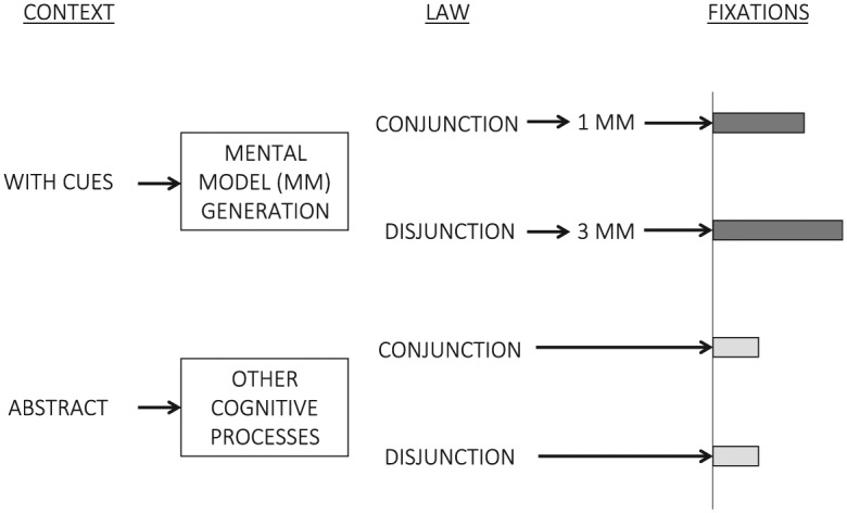
Visual representation of the cognitive processes involved in each condition and predictions for the outcome variable in each condition.
Strategy 2: Visual Representation of Data Distributions and Choice of the Appropriate Distribution for Analysis
A rather underused but exciting approach in data analysis is that of GAMLSS (Rigby & Stasinopoulos, 2001; Stasinopoulos & Rigby, 2007). GAMLSS stands for Generalized Additive Models for Location, Scale, and Shape. The goal of this method is to relax distributions’ hypotheses’ assumptions to fit more realistic theoretical distributions to the response variables. This is achieved by using extra information from the location, scale, and shape parameters (e.g., skewness and kurtosis). In this way GAMLSS can be seen as a tool to exploratory data analysis (e.g., Tukey, 1969). This method can be extended by modelling the response variable in order to find the type of distribution that best represents the data, thus providing the foundations for further analyses.
For example, this method has been useful in identifying mixture distributions that describe density estimates of forests (Jaskierniak, Lane, Robinson, & Lucieer, 2011), in describing distributions that fit data from the mini-mental state examination test (Muñiz-Terrera, van den Hout, Rigby, & Stasinopoulos, 2016), and in modelling handgrip strength in children (D. Cohen et al., 2010). Indeed, it has been shown that GAMLSS offers better fits of effects on transformed and untransformed body mass index data than traditional generalized linear models (Beyerlein, Fahrmeir, Mansmann, & Toschke, 2008).
The first step in GAMLSS modelling is to propose a marginal parametric distribution of the response variable in order to visualize subsets of independent variables and their relationships. This marginal distribution analysis aids understanding of the effects of single independent variables as well as combinations of independent variables on the response variable. Based on the visual inspection of different types of distributions fitting the data, the researcher can select the most appropriate distribution to be used in a statistical analysis of that data. Alternatively, as shown in our worked example, the researcher may use model comparison measures (e.g., Akaike information criterion [AIC], Bayesian information criterion [BIC]) to choose the most appropriate type of distribution.
Moreover, in GAMLSS models with different probability distributions, trends in the parameters and change points in mean and/or variance can be compared. These will provide additional evidence for the presence (or absence) of abrupt and/or slowly varying changes. These features reveal GAMLSS into an explanatory tool for finding appropriate set of models to describe the behavior of data.
Strategy 3: Model Comparison
Rodgers (2010) stated that there has been a quiet methodological revolution based on modelling. This is also shown in some textbooks: Data Analysis: A Model Comparison Approach (Judd & McClelland, 1989; Judd, McClelland, & Ryan, 2011) and Designing Experiments and Analyzing Data: A Model Comparison Approach (Maxwell & Delaney, 1990). Rodgers suggested that “[t]he methodological revolution . . . has involved the transition from the NHST paradigms developed by Fisher and Neyman-Pearson to a paradigm based on building, comparing, and evaluating statistical/mathematical models” (Rodgers, 2010, p. 3). The modelling approach involves developing models derived from theories and comparing those models on how well they fit the data using some measure (e.g., AIC, BIC, as mentioned above) that takes into account both how well the model fits the data and the complexity of the model (see Breiman, 2001, and McCullagh, 2002, for full-length discussions on modelling).
In this strategy, NHST is one of many possible model comparisons. In NHST, the model of the researcher (i.e., the alternative hypothesis) is compared to some model of chance (i.e., the null hypothesis). In the model comparison strategy, researchers may compare nested models (i.e., comparison between a model and a simpler version of that model) or nonnested models. An example of comparing nested models would be research that aims to determine whether there is a correlation between academic performance and numbers of hours of study. The researcher’s model may include academic performance as the outcome variable and number of hours of study as the predictor variable, with some variability in academic performance due to chance. The chance model is one in which academic performance is all due to chance. These two models are nested because the chance model is a simpler version of the researcher’s model. An alternative is to compare the researcher’s model with an alternative model in which the number of hours of study is ignored, and academic performance is predicted only by the age (in months) of the students. These models are not nested because none of them is a simpler version of the other.
There are numerous approaches that utilize model comparison, including the following: generalized linear models (GLM; Nelder & Wedderburn, 1972), SEM (Kline, 2011; Loehlin, 2011), multilevel analysis (MLV; Browne & Rasbash, 2004), Bayesian analysis such as Bayes factor comparison (BF; Berger & Pericchi, 1996; De Santis & Spezzaferri, 1997; Gelman, Carlin, Stern, & Rubin, 2003), Bayesian hierarchical models (Craigmile, 2009; Rossi, Allenby, & McCulloch, 2005), generalized estimating equations (GEE; Hardin & Hilbe, 2003), recursive partitioning methods (Strobl, Malley, & Tutz, 2009; Zeileis, Hothorn, & Hornik, 2008), linear quantile mixed models (LQMM; Geraci & Bottai, 2014), and LASSO regression (Tibshirani, 1996, 1997). We now illustrate the three strategies with a worked example.
Worked Example
We used a data set of 34 participants who completed reasoning tasks under four conditions. Measures of accuracy, reaction time, and eye fixation times were obtained; but here we only use the fixation time data.1 For more details about the research design and methods, see Macbeth et al. (2014). Participants solved reasoning problems in two contexts (with cues and abstract). Within each context, there were two types of reasoning problems regarding the type of law they used (conjunction and disjunction). The predictions of this study are presented in the next section. They are derived from the theory of mental models (Johnson-Laird, 1983).
Figure 1 shows boxplots representing the fixation times in each condition overlaid on the data of each participant in each condition.
Figure 1.

Distribution of reaction times in the four conditions, represented with boxplots for each condition and with the data of each individual in each condition (notches around the median represent approximate 95% confidence intervals).
Strategy 1: Visual Representation of Cognitive Processes and Predictions
Figure 2 shows the visual representation of the hypothesized cognitive processes involved in solving the reasoning problems for each condition, and a predicted qualitative pattern of values for the outcome variable fixation time. In the first column there are two context conditions (with cues and abstract). The figure indicates that in the context with cues participants are capable of generating mental models while they try to solve the reasoning problems. On the other hand, in the abstract context condition it is assumed that the participants are not able to generate mental models while they try to solve the reasoning problems. Within each context the participants were requested to solve problems with a conjunction rule and with a disjunction rule. In the context with cues, it is assumed that the participants generate only one mental model when solving problems with a conjunction rule and three mental models when they solve problems with a disjunction rule.
In the last column the figure presents barplots, which represent the predictions of the researcher regarding fixation time. The dark grey bars represent the predicted pattern for problems in the context with cues, suggesting that, due to the need to generate three mental models of the problem, the participants’ fixation times would be longer than those in the conjunction condition. The light gray bars represent the predicted pattern for problems in the abstract context. Given that the participants are not generating mental models, the fixation time would be shorter than in the context with cues and would not show any difference between the conjunction and disjunction conditions. In our worked example, we represent two categorical variables and one numerical variable, but the same approach could be used in other situations. For example, in the case of one categorical and two numerical variables, the graph would have an X axis and a Y axis, and the hypothesis would be represented with a trend line (linear or nonlinear) for each category. Three numerical variables could also be presented in a graph with an X axis and a Y axis, and the hypothesis could be represented as magnitudes of the third variable with squares of different sizes on several values of the other two variables (for an example, see Shiffrin, Lee, Kim, & Wagenmakers, 2008, Figure 3).
Figure 3.

Probability density functions of the selected conditional responses. “A” shows the (nonparametric) kernel density estimate of distribution of responses (“fixation time” in ms) to the two-level factor “law” (“negative conjunction” and “negative disjunction”) in the two-level factor “context” (“abstract” and “with cue”). “B” shows the distribution of responses (“fixation time” in ms) given to each set of four items (Items 1-4 and 4-8) used in each “law” factor. The first row in “B” shows the density plots shown in the left panel of “A” as separate plots. The second row in “B” shows the density plots shown in the right panel of “A” (“Y” corresponds to “fixation time”). In addition to the kernel densities, the (parametric) density function (solid) lines of the distributions fitted to the conditional responses are also shown. In all cases, the actual observations are shown as “rugs” in the X axis. “C” shows the RTs associated to each of the four experimental items in each “law” condition.
Strategy 2: Visual Representation of Data Distributions and Choice of the Appropriate Distribution for Analysis
For the sake of brevity, we focus on the case of the effects of the independent variables “context” and “law” on the response variable; the case of “item” and “law” is shown to further illustrate the way data distribute (see Figure 3). These plots reveal interesting behavior in the data. For example, Figure 3A and B not only show that data have a positive skew but also that there seems to be some multimodality. Figure 3C displays how RTs (reaction times) distribute for each experimental item in each condition. The parametric Gamma distribution fitted the data best (see Table 1), and its density significantly overlapped that of the (nonparametric) Kernel density estimation. These graphical results evidence that the distributional assumption (i.e., the Gamma distribution) is appropriate.
Table 1.
Fitted Values of Six Distributions When Fitted to Four Conditional Responses.
| Distribution |
||||||
|---|---|---|---|---|---|---|
| Conditional response | Normal | Ex-Gaussian | Weibull | Log-normal | Gamma | Gumbel |
| Y | context = abstract, law = negative conjunction | 2606.391 [2612.217] | 2577.956 [2586.694] | 2579.473 [2585.298] | 2575.598 [2581.423] | 2573.227 [2579.052] | 2660.631 [2666.456] |
| Y | context = abstract, law = negative disjunction | 2559.077 [2564.902] | 2529.083 [2537.821] | 2540.034 [2545.859] | 2525.525 [2531.350] | 2527.435 [2533.260] | 2622.958 [2628.784] |
| Y | context = with cues, law = negative conjunction | 2650.538 [2656.363] | 2648.110 [2656.848] | 2646.153 [2651.978] | 2671.207 [2677.033] | 2651.600 [2657.425] | 2692.538 [2698.363] |
| Y | context = with cues, law = negative disjunction | 2680.437 [2686.262] | 2670.777 [2679.515] | 2672.717 [2678.543] | 2678.367 [2684.193] | 2668.807 [2674.633] | 2723.768 [2729.593] |
| Median AIC [Median BIC] | 2628.464 [2634.29] | 2613.033 [2621.771] | 2612.813 [2618.638] | 2623.402 [2629.228] | 2612.413 [2618.239] | 2676.584 [2682.41] |
Note. AIC = Akaike information criterion; BIC = Schwarz Bayesian information criterion; the lower these values, the better the fitting. “Y” corresponds to the dependent variable (“fixation times” in this case). The lowest AIC values for each conditional response are shaded. The average AIC values given by the distributions across conditional responses are shown in the last row and the lowest AIC values appear in bold.
The graphics suggest that linear (mixed-effects) modelling is not appropriate, since the conditional distribution of the responses is not normal. Alternatives include normalizing the data via transformations (e.g., Vélez, Correa, & Marmolejo-Ramos, 2015) and carrying on with the linear modelling; modelling the data using generalized linear (mixed-effects) models and using a family of positively skewed distributions. By applying normality tests to the conditional distributions, it could be evidenced that the data do not distribute normally. However, it is more interesting to know what nonnormal distribution better represents the data. Table 1 shows the results of fitting five candidate distributions. The normal distribution is included to substantiate that the data are not normal.
The results not only indicate that a normal distribution does not fit the data well but that a Gamma distribution should be used to model the data. Thus, a complementary analysis to that presented earlier could consist of modelling the response variable via Gamma distributions. Although location (e.g., mean) shifts are routinely considered “the” measure of effect, it is also possible that a causal factor manifests primarily through heteroscedasticity (i.e., variation) in data. That is, most researchers aim at comparing averages, which usually sit in the peak (or thereabouts) of a distribution, via location tests (e.g., t test). However, such tests ignore other distributional aspects such as scale (i.e., variability; skewness and kurtosis), and heavy tails.2 These parameters are also theoretically and substantively important in their own right and should be used for more comprehensive distributional analyses.3 Thus, an additional analysis could focus on scale and shape parameters of the response variable in terms of the distribution that best fits the data (in the current example, the Gamma distribution).4
Strategy 3: Model Comparison
The model comparison strategy used in this worked example is multilevel analysis. A detailed description of this strategy is beyond the scope of this article (for detailed explanations of multilevel analysis, see Browne & Rasbash, 2004; Hox, 2010). Multilevel analysis was originally developed to deal with survey or archival data that contained two or more levels. For example, studies investigating academic performance of students at different schools in different cities have three levels: students, schools, and cities. The academic performance outcome variable may be partially explained by variations at different levels: students’ hours of study, academic ranking of schools, and/or political affiliation of the mayor of each city. Unlike one-level models in which the variability of the outcome variable is explained by the predictor(s) variable(s) and some random variability, in multilevel analysis there is random variability at each level. In this case, students, school, and cities are considered random factors.
Hoffman (2007) proposed that multilevel analysis could be used in psychology experiments. One of the advantages of this approach is that psychological experiments frequently utilize within-subjects designs, which creates problems in terms of independence of observations. An obvious application of the multilevel analysis is to use subjects as a random factor, in order to take into account the variability between individuals. Moreover, if several measures are obtained for items, items could also be considered a random factor. Note, however, that in our worked example we only use subjects as a random factor.
Our worked example was built on the information obtained in the GAMLSS approach, which indicated that the Gamma distribution is the most appropriate to fit the data. Therefore, in our multilevel analysis we used a generalized linear model (GLM) instead of a more typical linear model.5 For inference purposes in the linear regression model, the data are assumed to be random and normally distributed, whereas in GLM, we use a distribution of the exponential family—the Gamma distribution (see more details in McCullagh & Nelder, 1989; Nelder & Wedderburn, 1972). Table 2 shows the multilevel analysis using the normal distribution, and Table 3 shows the multilevel analysis using the Gamma distribution. (The analysis was conducted with the package lme4 [Bates, 2010] in the statistical software R [R Core Team, 2015].) In all the models, the AIC was lower in the Gamma distribution analysis than in the normal distribution analysis, thus dismissing the idea of the data distributing normally.
Table 2.
Multilevel Analysis: Normal Distribution.
| Parameter | Model 1 | Model 2 | Model 3 | Model 4 | Model 5 |
|---|---|---|---|---|---|
| Fixed effects | |||||
| Intercept | 6.151 [0.4] | 8.019 [0.4] | 5.889 [0.4] | 6.243[0.5] | 6.243 [0.5] |
| Context | 4.261 [0.3] | 4.261 [0.3] | 3.553 [0.4] | 3.553 [0.5] | |
| Law | 0.525 [0.3] | 0.525 [0.3] | −0.183 [0.4] | −0.183 [0.4] | |
| Context × Law | 1.416 [0.5] | 1.416 [0.5] | |||
| Variance components | |||||
| Participant variance | |||||
| Intercept | 4.843 (2.2) | 4.545 (2.1) | 4.847 (2.2) | 4.856 (2.2) | 3.482 (1.9) |
| Context | 5.065 (2.3) | ||||
| Residual variance | 9.748 (3.1) | 14.515 (3.8) | 9.674 (3.1) | 9.540 (3.1) | 8.189 (2.9) |
| Fit statistics | |||||
| AIC | 2865 | 3068.1 | 2863.1 | 2858 | 2819.3 |
Note. AIC = Akaike information criterion. The standard error of the estimates of the fixed effects are within brackets. As indicated by Bates (2010) we can only report the standard deviation, in parentheses, for the random effects. The shade indicates the lowest AIC.
Table 3.
Multilevel Analysis: Gamma Distribution.
| Parameter | Model 1 | Model 2 | Model 3 | Model 4 | Model 5 |
|---|---|---|---|---|---|
| Fixed effects | |||||
| Intercept | 6.471 [0.5] | 8.099 [0.5] | 6.277 [0.5] | 6.397 [0.5] | 6.390 [0.5] |
| Context | 4.114 [0.3] | 4.092 [0.3] | 3.552 [0.4] | 3.782 [0.6] | |
| Law | 0.658 [0.3] | 0.423 [0.2] | 0.166 [0.2] | 0.282 [0.2] | |
| Context × Law | 1.12 [0.5] | 1.051 [0.5] | |||
| Variance components | |||||
| Participant variance | |||||
| Intercept | 1.755 (1.3) | 2.296 (1.5) | 1.768 (1.3) | 1.75 (1.3) | 1.815 (1.3) |
| Context | 3.501 (1.9) | ||||
| Residual variance | 0.154 (0.4) | 0.213 (0.4) | 0.153 (0.4) | 0.151 (0.4) | 0.138 (0.4) |
| Fit statistics | |||||
| AIC | 2739 | 2950.5 | 2737.2 | 2734.6 | 2682.1 |
Note. AIC = Akaike information criterion. The standard error of the estimates of the fixed effects are within brackets. As indicated by Bates (2010) we can only report the standard deviation, in parentheses, for the random effects. The shade indicates the lowest AIC.
Following are the models we compared in both distributions. A null model (not shown in Tables 2 and 3), which is a one-level linear model that did not estimate the variability of the intercept between participants, with AIC = 3007.9. Model 1 incorporated an intercept and the effect of context on fixation times. Moreover, it estimated the variability of the intercept between participants. Given that Model 1, which includes variability between participants in the intercept, has a lower AIC than the null model in all the other models, the variability of the intercept between participants was estimated. Model 2 estimated the effect of law (but not context) on fixation times. The AIC is much higher than that in Model 1, indicating that context was the stronger predictor of fixation times. But, given that its AIC is lower than that of the null model, we kept law in the subsequent models. Model 3 incorporated both context and law. The AIC is lower than that of Model 1, confirming that both variables are important to predict fixation times.
Model 4 added the interaction between context and law. The AIC was lower than that of Model 3, indicating that the interaction context × law is important. Finally, Model 5 estimated the variability of the effect of context between participants. The AIC is significantly lower than that of Model 4. We tried other combinations of parameters, but Model 5 is the one that led to a lower AIC. Thus, the evidence is in favor of a model that takes into account the variables context and law, their interaction as fixed effects, the variability of the intercept and the context effect, and the residuals, as random effects.
Discussion
We presented three strategies that could be used to replace the NHST approach: (1) visual representation of cognitive processes and predictions, (2) visual representation of data distributions and choice of the appropriate distribution for analysis, and (3) model comparison. The first strategy provides the reader with a visual representation of the theories underlying the study and the predictions derived from the theories. We conclude that making a visual representation of the theories and the predictions not only facilitates the reader’s understanding of the study but may also improve research design. Producing a visual representation of a theory and its predictions in the process of designing a study may help the researcher choose more appropriate variables, operationalize variables, and control confounding variables.
Likewise, the second strategy is useful for the reader’s comprehension of the characteristics of the data and for choosing appropriate analytical tools. As shown in the worked example, the GAMLSS analysis identified the appropriate distribution to use in the multilevel analysis. Finally, the third strategy—model comparison—is useful as an analytical tool to replace NHST. Moreover, it may assist the researcher in the selection of a model for designing theoretically based studies. Although it could be beneficial to apply the three strategies after a study has been conducted, we encourage researchers to implement these strategies at the design stage.
The purpose of this article was to go beyond the stage of criticisms to NHST and provide strategies to replace this approach. We hope this article provides useful tools to encourage psychologists to look beyond NHST when designing research, analyzing data, and presenting their results.
Acknowledgments
The authors thank Susan Brunner for proofreading this article.
The data set and the R code for the analysis presented in Strategies 2 and 3 can be accessed freely at https://dx.doi.org/10.6084/m9.figshare.2413291.v2
Note that a simple alternative of analysis that combines measures of location and scale can be done via the coefficient of variation (for the case of normally distributed data: ) or the coefficient of quartile variation (for the case of nonnormally distributed data: ) and confidence intervals around them (Bonett, 2006) incidentally, the formula for Cqv is mistyped in Bonett’s article. Intuitively, another robust measure could be obtained by using the median and its associated measure of variability: Cmv =MAD/Mdn. This is a measure of relative dispersion that can be used to compare dependent and independent data sets. It is rarely seen in psychological research.
Earlier work focusing on comparing distributions can be seen in the probability plots (Wilk & Gnanadesikan, 1968) and the Ordinal Dominance curve (Darlington, 1973).
If the model contains one or more continuous covariates, then their graphical representation would look like a usual correlation plot (in the case of a bivariate plot); for example, “participants’ age” (PA) in the Y axis and RTs in the X axis. A graphical enhancement would be done by adding marginal density plots by the X and Y axes (for a recent example, see Open Science Collaboration, 2015, Figure 3). Another approach would be to discretize a continuous variable to create categories and then to establish density plots for each category. In the example above, PA can be discretized via a median split in order to generate two categories, that is, Age Group 1 < median(PA) and Age Group 2 > median(PA). Subsequently, the X axis could represent the RTs for each of the two age groups while the Y axis would be the distribution’s density. Note that although discretizing continuous variables is not recommended (e.g., Altman & Royston, 2006), it could be considered as an option only if strictly required.
Empirical evidence shows that GLMs have more power than traditional linear models (e.g., ANOVA) even though they might lead to the same conclusions (see Moscatelli, Mezzetti, & Lacquaniti, 2012). A recent method known as automated mixed ANOVA modelling implements backward elimination of nonsignificant random and fixed effects and gives the results in ANOVA terms (Kuznetsova, Christensen, Bavay, & Brockhoff, 2015). This method is thus a balanced blend between GLM and ANOVA procedures.
Footnotes
Declaration of Conflicting Interests: The author(s) declared no potential conflicts of interest with respect to the research, authorship, and/or publication of this article.
Funding: The author(s) received no financial support for the research, authorship, and/or publication of this article.
References
- Altman D. G., Royston P. (2006). The cost of dichotomising continuous variables. British Medical Journal, 332, 1080. [DOI] [PMC free article] [PubMed] [Google Scholar]
- Anderson J. R., Bothell D., Byrne M. D., Douglass S., Lebiere C., Qin Y. (2004). An integrated theory of the mind. Psychological Review, 111, 1036-1060. [DOI] [PubMed] [Google Scholar]
- Bates D. M. (2010). lme4: Mixed-effects modelling with R. Madison, WI: Springer. [Google Scholar]
- Berger J. O., Pericchi L. R. (1996). The intrinsic Bayes factor for model selection and prediction. Journal of the American Statistical Association, 91, 109-122. [Google Scholar]
- Beyerlein A., Fahrmeir L., Mansmann U., Toschke A. M. (2008). Alternative regression models to assess increase in childhood BMI. BMC Medical Research Methodology, 8, 59. doi: 10.1186/1471-2288-8-59 [DOI] [PMC free article] [PubMed] [Google Scholar]
- Bezerra R. F., Jalloh S., Stevenson J. (1998). Formulating hypothesis graphically in social research. Quality & Quantity, 32, 327-353. [Google Scholar]
- Bonett D. G. (2006). Confidence interval for a coefficient of quartile variation. Computational Statistics & Data Analysis, 50, 2953-2957. [Google Scholar]
- Breiman L. (2001). Statistical modelling: The two cultures. Statistical Science, 16, 199-231. [Google Scholar]
- Browne W., Rasbash J. (2004). Multilevel modelling. In Hardy M., Bryman A. (Eds.), Handbook of data analysis (pp. 459-480). London, England: Sage. [Google Scholar]
- Campitelli G., Gerrans P. (2014). Does the cognitive reflection test measure cognitive reflection? A mathematical modeling approach. Memory & Cognition, 42, 434-447. [DOI] [PubMed] [Google Scholar]
- Campitelli G., Macbeth G. (2014). Hierarchical graphical Bayesian models in psychology. Revista Colombiana de Estadística, 37, 319-339. [Google Scholar]
- Cohen D., Voss C., Taylor M., Stasinopoulos D. M., Delextrat A., Sandercock G. (2010). Handgrip strength in English schoolchildren. Acta Paediatrica, 99, 1065-1072. [DOI] [PubMed] [Google Scholar]
- Cohen J. (1994). The earth is round (p < .05). American Psychologist, 49, 997-1003. [Google Scholar]
- Craigmile P. (2009). Hierarchical model building, fitting, and checking: A behind-the-scenes look at a Bayesian analysis of arsenic exposure pathways. Bayesian Analysis, 4, 1-36. [Google Scholar]
- Darlington R. B. (1973). Comparing two distributions via simple graphs. Psychological Bulletin, 79, 110-116. [Google Scholar]
- De Santis F., Spezzaferri F. (1997). Alternative Bayes factors for model selection. Canadian Journal of Statistics, 25, 503-515. [Google Scholar]
- Gelman A., Carlin J. B., Stern H. S., Rubin D. B. (2003). Bayesian data analysis. London, England: Chapman & Hall/CRC Press. [Google Scholar]
- Geraci M., Bottai M. (2014). Linear quantile mixed models. Statistics and Computing, 24, 461-479. [Google Scholar]
- Hardin J., Hilbe J. (2003). Generalized estimating equations. London, England: Chapman & Hall/CRC Press. [Google Scholar]
- Hoffman L. (2007). Multilevel models for examining individual differences in within-person variation and covariation over time. Multivariate Behavioral Research, 42, 609-629. [Google Scholar]
- Hox J. J. (2010). Multilevel analysis: Techniques and applications (2nd ed.). New York, NY: Routledge. [Google Scholar]
- Jaskierniak D., Lane P., Robinson A., Lucieer A. (2011). Extracting LiDAR indices characterise multilayered forest structure using mixture distribution function. Remote Sensing of Environment, 115, 573-585. [Google Scholar]
- Johnson-Laird P. N. (1983). Mental models: Towards a cognitive science of language, inference, and consciousness. Cambridge, MA: Harvard University Press. [Google Scholar]
- Jordan M. I. (2004). Graphical models. Statistical Science, 19, 140-155. [Google Scholar]
- Judd C. M., McClelland G. H. (1989). Data analysis: A model comparison approach. Orlando, FL: Harcourt Brace Jovanovich. [Google Scholar]
- Judd C. M., McClelland G. H., Ryan C. S. (2011). Data analysis: A model comparison approach (2nd ed.). New York, NY: Routledge. [Google Scholar]
- Kline R. B. (2011). Principles and practice of structural equation modeling (3rd ed.). New York, NY: Guilford. [Google Scholar]
- Koller D., Friedman N., Getoor L., Taskar B. (2007). Graphical models in a nutshell. In Getoor L., Taskar B. (Eds.), Introduction to statistical relational learning (pp. 13-56). Cambridge: MIT Press. [Google Scholar]
- Kuznetsova A., Christensen R., Bavay C., Brockhoff P. (2015). Automated mixed ANOVA modelling of sensory and consumer data. Food Quality and Preference, 40, 31-38. [Google Scholar]
- Lee M. D. (2008). Three case studies in the Bayesian analysis of cognitive models. Psychonomic Bulletin and Review, 15, 1-15. [DOI] [PubMed] [Google Scholar]
- Loehlin J. C. (2011). Latent variable models: An introduction to factor, path, and structural equation analysis (4th ed.). New York, NY: Routledge. [Google Scholar]
- Macbeth G., Razumiejczyk E., Crivello M. E., Bolzán C., Pereyra C. I., Campitelli G. (2014). Mental models of the negation of conjunctions and disjunctions. Europe’s Journal of Psychology, 10, 135-149. [Google Scholar]
- Maxwell S. E., Delaney H. D. (1990). Designing experiments and analyzing data: A model comparison approach. Belmont, CA: Wadsworth. [Google Scholar]
- McCullagh P. (2002). What is a statistical model? Annals of Statistics, 30, 1225-1310. [Google Scholar]
- McCullagh P., Nelder J. A. (1989). Generalized linear models (2nd ed.). London, England: Chapman & Hall. [Google Scholar]
- Moscatelli A., Mezzetti M., Lacquaniti F. (2012). Modelling psychophysical data at the population-level: The generalized linear mixed model. Journal of Vision, 12, 11. doi: 10.1167/12.11.26 [DOI] [PubMed] [Google Scholar]
- Muñiz-Terrera G., van den Hout A., Rigby R. A., Stasinopoulos D. M. (2016). Analysing cognitive test data: Distributions and non-parametric random effects. Statistical Methods in Medical Research, 25, 741-753. doi: 10.1177/0962280212465500 [DOI] [PubMed] [Google Scholar]
- Nelder J.A., Wedderburn R. W. M. (1972). Generalized linear models. Journal of the Royal Statistical Society, Series A, 135, 370-384. [Google Scholar]
- Open Science Collaboration. (2015). Estimating the reproducibility of psychological science. Science, 349(6251), aac4716. doi: 10.1126/science.aac4716 [DOI] [PubMed] [Google Scholar]
- Pearl J. (2009). Causal inference in statistics: An overview. Statistics Surveys, 3, 96-146. [Google Scholar]
- R Core Team. (2015). R: A language and environment for statistical computing. Vienna, Austria: R Foundation for Statistical Computing; Retrieved from http://www.R-project.org/ [Google Scholar]
- Rigby R. A., Stasinopoulos D. M. (2001). The GAMLSS project: A flexible approach to statistical modelling, In Klein B., Korsholmn L. (Eds.), New trends in statistical modelling: Proceedings of the 16th International Workshop on Statistical Modelling (pp. 337-345). Odense, Denmark. [Google Scholar]
- Rodgers J. L. (2010). The epistemology of mathematical and statistical modeling: A quiet methodological revolution. American Psychologist, 65, 1-12. [DOI] [PubMed] [Google Scholar]
- Rossi P. E., Allenby G. M., McCulloch R. (2005). Bayesian statistics and marketing. New York, NY: Wiley-Interscience. [Google Scholar]
- Shiffrin R. M., Lee M. D., Kim W., Wagenmakers E. J. (2008). A survey of model evaluation approaches with a tutorial on hierarchical Bayesian methods. Cognitive Science, 32, 1248-1284. [DOI] [PubMed] [Google Scholar]
- Stasinopoulos D. M., Rigby R. A. (2007). Generalized additive models for location scale and shape (GAMLSS) in R. Journal of Statistical Software, 23, 1-46. [Google Scholar]
- Strobl C., Malley J., Tutz G. (2009). An introduction to recursive partitioning: Rationale, application and characteristics of classification and regression trees, bagging and random forests. Psychological Methods, 14, 323-348. [DOI] [PMC free article] [PubMed] [Google Scholar]
- Tibshirani R. (1996). Regression shrinkage and selection via the LASSO. Journal of the Royal Statistical Society, Series B, 58, 267-288. [Google Scholar]
- Tibshirani R. (1997). The LASSO method for variable selection in the Cox model. Statistics in Medicine, 16, 385-395. [DOI] [PubMed] [Google Scholar]
- Tukey J. W. (1969). Analysing data: Sanctification or detective work? American Psychologist, 24, 83-91. [Google Scholar]
- Vélez J. I., Correa J. C., Marmolejo-Ramos F. (2015). A new approach to the Box-Cox transformation. Frontiers in Applied Mathematics and Statistics, 1, 12. [Google Scholar]
- Wagenmakers E.-J. (2007). A practical solution to the pervasive problems of p values. Psychonomic Bulletin and Review, 14, 779-804. [DOI] [PubMed] [Google Scholar]
- Wilk M. B., Gnanadesikan R. (1968). Probability plotting methods for the analysis of data. Biometrika, 55, 1-17. [PubMed] [Google Scholar]
- Zeileis A., Hothorn T., Hornik K. (2008). Model-based recursive partitioning. Journal of Computational and Graphical Statistics, 17, 492-514. [Google Scholar]