

Abstract
Student Growth Percentiles (SGPs) increasingly are being used in the United States for inferences about student achievement growth and educator effectiveness. Emerging research has indicated that SGPs estimated from observed test scores have large measurement errors. As such, little is known about “true” SGPs, which are defined in terms of nonlinear functions of latent achievement attributes for individual students and their distributions across students. We develop a novel framework using latent regression multidimensional item response theory models to study distributional properties of true SGPs. We apply these methods to several cohorts of longitudinal item response data from more than 330,000 students in a large urban metropolitan area to provide new empirical information about true SGPs. We find that true SGPs are correlated 0.3 to 0.5 across mathematics and English language arts, and that they have nontrivial relationships with individual student characteristics, particularly student race/ethnicity and absenteeism. We evaluate the potential of using these relationships to improve the accuracy of SGPs estimated from observed test scores, finding that accuracy gains even under optimal circumstances are modest. We also consider the properties of SGPs averaged to the teacher level, widely used for teacher evaluations. We find that average true SGPs for individual teachers vary substantially as a function of the characteristics of the students they teach. We discuss implications of our findings for the estimation and interpretation of SGPs at both the individual and aggregate levels.
Keywords: academic growth, ability estimation, Bayesian estimation, auxiliary information, teacher value-added
A Student Growth Percentile (SGP) is the percentile rank of a student’s current achievement among students with similar prior achievement (Betebenner, 2009). For example, a student whose current achievement is at the 70th percentile among students matched to him/her with respect to prior achievement would have an SGP equal to 70. Two features of this definition make SGPs appealing. First, the percentile rank scale is familiar and interpretable, and remains well-defined even if test scores are not vertically or even intervally scaled (Betebenner, 2009; Briggs & Betebenner, 2009; Castellano & Ho, 2013). Second, ranking students against other students with similar prior achievement is perceived as more fair and relevant to evaluating both individual student progress and educator effectiveness than simply examining unadjusted achievement levels (Betebenner, 2009). These benefits have contributed to the increasing use of SGPs in the United States.
However, recent research has demonstrated that SGPs estimated from standardized test scores suffer from large estimation errors (Akram, Erickson, & Meyer, 2013; Lockwood & Castellano, 2015; McCaffrey, Castellano, & Lockwood, 2015; Monroe & Cai, 2015; Shang, Van Iwaarden, & Betebenner, 2015). Both the prior and current test scores used in SGP calculations are error-prone measures of their corresponding latent achievement traits due to the finite number of items on each test (Lord, 1980). These errors combine to make estimated SGPs noisy measures of the “true” (or latent) SGPs, defined for each student as the percentile rank of his/her current latent achievement among students with the same prior latent achievement (Lockwood & Castellano, 2015).
These errors jeopardize the validity of inferences made from estimated SGPs. For example, stakeholders and other consumers of SGP data are likely to be interested in students’ true SGPs as indicators of academic progress. However, McCaffrey et al. (2015) demonstrate that under typical testing conditions, 95% confidence intervals for true SGPs given estimated SGPs often cover much of the entire 0 to 100 percentile rank range. Thus, estimated SGPs typically are only weakly informative about actual academic progress for individual students. Moreover, the errors in estimated SGPs contain a component that is positively related to students’ true prior achievement levels (McCaffrey et al., 2015). This is problematic for interpreting SGPs aggregated to teacher or school levels as indicators of educator effectiveness, because it implies that aggregated SGPs for equally proficient educators who serve students of different prior achievement levels will tend to be different.
Understanding whether alternative ways of estimating SGPs from observed data could mitigate such problems depends on distributional properties of true SGPs that are currently unknown. For example, if true SGPs are correlated across tested subjects and/or with auxiliary data such as student background characteristics, shrinkage estimators that exploit these relationships can be used to improve accuracy of estimated SGPs (Efron & Morris, 1973). de la Torre (2009) makes analogous arguments for estimating latent abilities using testing data from multiple academic subjects, and Sinharay, Puhan, and Haberman (2011) review the extensive literature on the use of shrinkage to improve the accuracy of estimated subscores. However, the potential accuracy gains from shrinkage depend in part on the strength of the relationships among the latent quantities and auxiliary information, and we currently do not know how strongly correlated true SGPs are across academic subjects, nor do we know to what extent true SGP distributions vary as a function of student background characteristics. This information cannot be learned simply by studying estimated SGPs because of the random and systematic measurement errors they contain.
Distributional properties of true SGPs also have implications for the ability of alternative estimation methods to improve fairness of SGP measures. As noted, one of the purported advantages of SGPs is that by comparing conditional achievement status relative to students with similar prior achievement, they provide a fair assessment of student progress. Understanding to what extent true SGP distributions vary with respect to student background variables is important for understanding to what extent they actually level the playing field, and whether improvements in tests, SGP estimation methods, or both could ultimately remove any undesirable correlations of the measures with student background characteristics. For example, Shang et al. (2015) suggest the SIMEX method of measurement error correction to reduce the bias in teacher-level aggregated SGPs due to measurement error in the prior test scores. However, if true SGPs are correlated with student background characteristics such as ethnicity and economic status, corrections for test measurement error alone would be insufficient to remove potentially undesirable relationships between teacher performance indicators and student background.
To study these issues, we apply latent regression (e.g., Mislevy, Beaton, Kaplan, & Sheehan, 1992; von Davier & Sinharay, 2010) multidimensional item response theory (MIRT; e.g., Adams, Wilson, & Wang, 1997) models to longitudinal item response data from several cohorts of students from a large urban metropolitan area. In the Statistical Model section, we develop a model for latent achievement across grades and subjects that includes regressions on student covariates, and show how the model can be used to estimate population joint distributions of true SGPs. In the Data section, we describe our data sources and estimation cohorts, which include item response data from Math and English language arts (ELA) assessments in Grades 3 to 8 as well as a variety of student covariates. We then consider three research aims: (1) describe the properties of true SGPs, namely, cross-subject correlations and relationships with student covariates, by estimating latent regression models and true SGP distributions; (2) evaluate the potential gains in accuracy for estimating individual student true SGPs by using their relationships to other observable information; and (3) evaluate to what extent true SGPs aggregated to the teacher level would demonstrate relationships with student background characteristics. We address each of the aims in turn, describing their relevant methods and results in their own sections. Finally, we discuss further implications, limitations, and next steps in the Discussion section.
Statistical Model
This section specifies a model for latent achievement attributes, defines true SGPs under this model, and shows how their distributional properties can be assessed from data.
Latent Regression MIRT Model
For students in a target grade level , we observe a vector of item responses as well as a vector of covariates, and we denote the observed values for student by . We assume each student also has a vector of latent achievement traits . We assume each corresponds to a particular grade and subject test that measures for each student. In our applications, where corresponds to Grade ELA and math, respectively, and to Grade ELA and math, respectively. We assume that are independent and identically distributed with joint distribution in a target population.
The joint distribution can be factored as . We assume that item responses are conditionally independent of the covariates given so that . We specify with a MIRT model with item parameters , and use the notation to make clear the dependence on the item parameters. We specify using latent regression models for :
where are vectors of latent regression coefficients and is assumed to satisfy and where is a positive definite covariance matrix. Thus, depends on the parameters , a matrix, as well as , and we use the notation to make this dependence clear. Finally, is the distribution of the covariates in the population.
This model specification is typical for latent regression in a MIRT context. For example, it is used by de la Torre (2009). Also, although the National Assessment of Educational Progress involves a complex sampling and assessment design as well as a large number of covariates, it too uses the same latent regression MIRT model specification assumed here (Mislevy, Johnson, & Muraki, 1992; von Davier & Sinharay, 2010).
SGP Definition
The true SGPs are defined as functions of , where the functions are derived from conditional distributions determined by the distribution of in the population. Let be an element of and be any other subset of that does not contain . For example, may correspond to a current math score ( in our example) and may correspond to a prior year math score ( in our example). We define the true SGP for given as , where is the conditional cumulative distribution function (CDF) of given , and are specific values of . In other words, is the percentile rank of in the conditional distribution of among individuals in the population for whom . By standard properties of CDFs (e.g., Theorem 2.1.4 of Casella & Berger, 1990), the random variable is uniformly distributed for each , and therefore is also uniformly distributed.
Our interest is in more complicated properties of the distribution of , such as its relationships with covariates . We thus require a method for computing this random variable. Standard probability manipulations give that
Conditioning on in Equation 2 simplifies the computations because has a multivariate normal distribution conditional on . The appendix shows how this distributional property permits for any to be computed easily given and . As described in the following section, the ability to compute as a function of allows us to infer distributional properties of true SGPs from .
Estimating Distributional Properties
Given data for , the likelihood function for the unknown parameters of the latent regression MIRT model is
This can be used to compute maximum likelihood estimates . The distribution can be estimated by plugging in for , and we denote this estimated distribution by . Likewise, the distribution can be estimated by plugging in for , and we denote this estimated distribution by . The data also provide an empirical distribution of the covariates that serves as an estimate of . Thus, the joint distribution can be estimated by
and this estimated distribution can be used to evaluate distributional properties of any functions of , including true SGPs.
We use Monte Carlo methods to assess distributional properties because they are simple to implement. To describe these methods, let refer to a vector of true SGPs of interest. In our application, we are primarily interested in corresponding to math SGPs and corresponding to ELA SGPs, so that . We can obtain samples from the estimated joint distribution of the true math SGPs, the true ELA SGPs, the covariates, and the item response data, denoted by , as follows. First, we obtain samples from by sampling from , then sampling from , and then sampling from . Second, we compute from for each sample, providing from . We can use these samples to compute any properties of , or any of its subdistributions such as , with arbitrary accuracy determined by the Monte Carlo sample size . For example, we can use the samples to compute conditional expectation functions such as or so that we can see to what extent groups of individuals with different covariates vary with respect to mean true SGPs under the model. We can likewise use the samples to compute . Finally, we can use them to compute conditional expectation functions for true SGPs given and/or various functions of to evaluate accuracy gains for estimating SGPs. These strategies, detailed in later sections, are used for all three of our research aims.
Data
For all analyses, we use longitudinal item-level data from a large, diversely populated city in the northeastern United States. We focus on the two most recent years of available data over which the testing program was stable: 2008-2009 (2009) and 2009-2010 (2010). We model data from both ELA and math to study the relationship of SGPs for the same student across these academic subjects. To address our aim of understanding the extent that true SGP distributions vary by student background variables, we consider key background variables that are supported by the available data.
We subset the data by students’ grade levels in 2010 for Grades 4 to 8, representing five 2010 grade-level cohorts. Each subset was a 2-year by 2-subject block with current and prior year data for both math and ELA. Table 1 summarizes the student distributions by our background covariates of interest for each cohort. None of the student background variables we consider vary by subject, and thus for each cohort, the frequencies and percentages refer to both ELA and math. We subset each cohort to students with item-level data for both subjects and years and with nonmissing records for each covariate, which resulted in attrition of between 9.5% and 11.4% of students by cohort. The final student sample sizes by cohort, at the bottom of Table 1, ranged from 65,093 to 67,343. Note that the table lists all covariates that we include in the latent regression model, and thus for each type of background variable, one of the categories is not shown but can easily be computed from the available frequencies in the table. For instance, for the Grade 4 cohort, 23% speak Spanish at home and 16% speak another non-English language at home, leaving 61% of students whose primary home language is English. For race/ethnicity, we combined Hispanic and Other as there was a relatively small proportion of students who identified themselves as “Other,” and preliminary analyses revealed they had similar performance across grades and subjects as Hispanic students.
Table 1.
Frequencies and Percentages of Students by Each Student Background Covariate for Each Cohort.
| Covariate | Grade 4 cohort |
Grade 5 cohort |
Grade 6 cohort |
Grade 7 cohort |
Grade 8 cohort |
|||||
|---|---|---|---|---|---|---|---|---|---|---|
| G3 2009 | G4 2010 | G4 2009 | G5 2010 | G5 2009 | G6 2010 | G6 2009 | G7 2010 | G7 2009 | G8 2010 | |
| Female | 33,130 (49%) | 33,130 (49%) | 32,258 (49%) | 32,258 (49%) | 32,198 (49%) | 32,198 (49%) | 31,889 (49%) | 3,188 (49%) | 32,583 (49%) | 32,583 (49%) |
| Asian | 10,048 (15%) | 10,048 (15%) | 9,277 (14%) | 9,277 (14%) | 9,178 (14%) | 9,178 (14%) | 9,278 (14%) | 9,278 (14%) | 9,586 (14%) | 9,586 (14%) |
| Hispanic or other | 26,750 (40%) | 26,750 (40%) | 26,646 (40%) | 26,646 (40%) | 26,421 (40%) | 26,421 (40%) | 26,144 (40%) | 26,144 (40%) | 26,363 (40%) | 26,363 (40%) |
| Black | 20,348 (30%) | 20,348 (30%) | 20,576 (31%) | 20,576 (31%) | 20,789 (32%) | 20,789 (32%) | 20,796 (32%) | 20,796 (32%) | 21,185 (32%) | 21,185 (32%) |
| Other home language | 10,493 (16%) | 10,493 (16%) | 10,059 (15%) | 10,059 (15%) | 9,996 (15%) | 9,996 (15%) | 10,412 (16%) | 10,412 (16%) | 10,708 (16%) | 10,708 (16%) |
| Spanish home language | 15,192 (23%) | 15,192 (23%) | 15,317 (23%) | 15,317 (23%) | 15,525 (24%) | 15,525 (24%) | 16,255 (25%) | 16,255 (25%) | 16,913 (25%) | 16,913 (25%) |
|
| ||||||||||
| ELL | 11,345 (17%) | 9,253 (14%) | 9,600 (15%) | 7,516 (11%) | 8,522 (13%) | 6,205 (9%) | 7,310 (11%) | 5,888 (9%) | 6,739 (10%) | 5,516 (8%) |
| Special education | 6,339 (9%) | 12,429 (18%) | 6,902 (10%) | 12,578 (19%) | 6,958 (11%) | 12,269 (19%) | 7,011 (11%) | 11,929 (18%) | 6,855 (10%) | 11,480 (17%) |
| Disability | 11,883 (18%) | 12291 (18%) | 12,350 (19%) | 12,361 (19%) | 12,181 (19%) | 12,112 (19%) | 11,898 (18%) | 11,747 (18%) | 11,539 (17%) | 11,303 (17%) |
| FRL | 42,162 (63%) | 58,417 (87%) | 41,367 (63%) | 57,301 (87%) | 41,062 (63%) | 55,499 (85%) | 44,349 (68%) | 55,199 (85%) | 43,918 (66%) | 55,778 (84%) |
| >10% absent | 13,346 (20%) | 11,056 (16%) | 12,965 (20%) | 10,969 (17%) | 12,651 (19%) | 12,251 (19%) | 14,116 (22%) | 13,880 (21%) | 15,759 (24%) | 17,240 (26%) |
|
| ||||||||||
| Total N | 67,343 | 67,343 | 66,064 | 66,064 | 65,350 | 65,350 | 65,093 | 65,093 | 66,368 | 66,368 |
We classify covariates as time-invariant or time-varying. The time-invariant covariates describe personal characteristics that remain static over time, including gender (female), race or ethnicity (Asian, Hispanic or Other, and Black), and home language spoken (Other Home Language and Spanish Home Language). The frequencies and percentages for these covariates, shown in the top half of the table, are thus the same for each year within each cohort. In contrast, the time-varying covariates that describe student statuses or group memberships can fluctuate over time. These covariates, shown in the bottom half the table, include English language learner (ELL) status, Special Education status, Disability status, Free or Reduced Price Lunch (FRL) status, and excessive school absences (>10%).
Generally, the distributions of time-varying covariates do not fluctuate substantially across the 2 years within a cohort with the exception of FRL status and Special Education status. The percentage of students coded as participating in FRL increased by between 17 and 24 percentage points for each cohort from 2009 to 2010, while the percentage of students coded as participating in Special Education programs increased by between 7 and 9 percentage points for each cohort from 2009 to 2010. Such changes were not explained in the data documentation, but perhaps shifts in eligibility and identification criteria were implemented over these years, resulting in increased participation in these programs.
Estimating Latent Regression Models and True SGP Distributions
In this section, we present details of how we fit the latent regression MIRT models to our data, and how we used the resulting parameter estimates to estimate properties of true SGP distributions. We then summarize these results.
Method
We model the latent achievement traits for the two years (2009 and 2010) and two subjects (ELA and math) jointly by covariates of interest (see Table 1) with a latent regression four-dimensional MIRT model. Separate models were fit for each of the five cohorts. The achievement tests include both dichotomously scored multiple choice and polytomously scored constructed-response items, which we model with a 2-parameter-logistic (2PL) and Generalized Partial Credit model (Muraki, 1992), respectively. No items are common across grade levels, so items for a particular grade-level and subject area load only on their corresponding dimension.1 That is, we have “between-item” MIRT models (Adams et al., 1997) for each current Grade cohort () with dimensions for achievement in ELA Grade (2009), math Grade (2009), ELA Grade (2010), and math Grade (2010).
We used the mixedmirt function in the mirt package (version 1.14; Chalmers, 2012) for the R environment (R Core Team, 2015) to compute maximum likelihood estimates for each cohort using the likelihood function in Equation 3. We used the Metropolis-Hastings Robbins-Monro (MH-RM) algorithm, which is well suited for large numbers of dimensions, items, and examinees (Cai, 2010).2 These conditions hold for our case, where for each cohort, there are dimensions, between 125 and 147 items across all four tests, and more than 65,000 students. To identify the model, we fixed all of the diagonal elements of to 1. We also grand-mean centered all covariates, precluding the need to estimate an overall intercept. Because the MH-RM algorithm is stochastic, its parameter estimates will not be identical across estimation runs for different starting seeds and values. To facilitate convergence, we fine-tuned modeling options (following correspondence with the mirt package author, Phil Chalmers), including using informed starting values for the latent regression coefficients. Specifically, we first fit separate unidimensional latent regression models for each latent trait and used their coefficient estimates as starting values in the full latent regression MIRT model.
As noted, the covariates for each student include both time-invariant and time-varying components. All time-invariant covariates (gender, race/ethnicity, home language) were included in each of the latent regressions in Equation 1. For the time-varying covariates (e.g., FRL and ELL status), we needed to decide whether the values from Grade would be included in only the math and ELA equations for Grade , or whether they would be included in all four equations. We needed to make an analogous decision for the values from Grade . We compared the “restricted” specification (where values of time-varying covariates were included in the equations for only their corresponding time point) to the “full” specification (where values of time-varying covariates from both time points were included in all four equations) using the Akaike Information Criterion (AIC). The AIC results overwhelmingly favored the full model for all five cohorts. Thus, we report all results using the full model.
For each cohort, we used the estimated model parameters and the Monte Carlo methods described previously to obtain samples from . We used samples for each cohort. There are three main sources of uncertainty in our inferences about conditional on the model specification. The first is sampling error in and due to the particular sample of students used for each cohort. The second is Monte Carlo error in due to the MH-RM algorithm. The third is Monte Carlo error in quantities computed from samples from . The combination of these sources of uncertainty has negligible consequences for the inferences reported in the rest of the article. Supporting evidence is provided in the appendix.
Latent Regression Results
Because we were using test score data that had already been calibrated for a state testing program, there were no apparent issues with the item parameter estimates or a need to drop misbehaving items. The latent regression coefficients, representing average group differences holding other covariates constant, generally followed patterns seen with test scores. For instance, we found negative relationships to latent achievement for Hispanic or Other, Black, ELL, Special Education, FRL, and excessive absences across all cohorts. For Asian, Other Home Language, and Spanish Home Language, we generally found small to moderate positive coefficients for both subjects. For females and Disability, relationships were not as consistent across subjects or time points: females generally had small negative coefficients for Math but small to moderate positive coefficients for ELA at both time points, and Disability tended to have positive coefficients for both subjects at Time 1 but negative coefficients at Time 2. Complete tables of the estimated latent regression coefficients by cohort and dimension are provided in the Supplemental Material (available online).
The covariates explain between 37% and 46% of the variance in the latent traits, depending on cohort and dimension. We compute this for each latent trait by
where for all due to the model identification constraint, and is computed with respect to . The Supplemental Material (available online) provides by cohort and dimension. The covariates tend to explain a larger percentage of the achievement variation for higher grades. For example, the average for the Grade 7 and 8 cohorts is 0.44, while that for the Grade 4 cohort is 0.39. It is worth noting that the relationships between the covariates and latent traits could be due in part to students with different background characteristics being taught by schools and teachers of different quality, a point we revisit later when trying to interpret relationships between true SGPs and student background.
The for each cohort are provided in Table 2. As the models were identified by fixing the residual variances to 1, the latent trait residual covariance matrices are also correlation matrices. The six pairwise correlations are ordered by pairs of residuals for latent traits with subject in common, then year in common, and last, nothing in common. Not surprisingly, residual correlations for traits that have something in common are higher than those with nothing in common (neither year nor subject) and are higher for common subjects (different years) than common years (different subjects).
Table 2.
Estimated Residual Correlations for Each Cohort.
| Cohort | Common subject |
Common year |
Nothing in common |
|||
|---|---|---|---|---|---|---|
| ELA 2009, ELA 2010 | Math 2009, Math 2010 | ELA 2009, Math 2009 | ELA 2010, Math 2010 | ELA 2009, Math 2010 | ELA 2010, Math 2009 | |
| 4 | 0.81 | 0.82 | 0.74 | 0.77 | 0.67 | 0.66 |
| 5 | 0.83 | 0.82 | 0.72 | 0.75 | 0.64 | 0.66 |
| 6 | 0.84 | 0.81 | 0.70 | 0.73 | 0.63 | 0.63 |
| 7 | 0.87 | 0.87 | 0.68 | 0.73 | 0.66 | 0.67 |
| 8 | 0.88 | 0.85 | 0.72 | 0.67 | 0.60 | 0.70 |
True SGP Distribution Results
We used samples from for each cohort to understand features of the true SGP distributions that may have implications for fairness of the measures as well as estimation accuracy. First, we are interested in the cross-subject correlations of the true SGPs, such as the correlation between Grade 4 ELA SGP given Grade 3 ELA achievement and Grade 4 math SGP given Grade 3 math achievement. These correlations are estimated to be 0.50, 0.52, 0.49, 0.30, and 0.36 for Grades 4 to 8, respectively. The positive correlations are consistent with the patterns from Table 2, which suggest a time-specific source of variance that affects both math and ELA achievement from the same grade. For example, if a student is having a particularly good year, he or she is likely to have true SGPs for both math and ELA that are above average. The smaller Grades 7 and 8 correlations may be due in part to the higher within-subject, cross-year correlations of the latent achievement traits in these grades compared to earlier grades, although the true SGP correlations are a complicated function of and so other factors are likely to be contributing.
The other key attribute of we examined was the extent to which true SGP distributions vary as a function of student characteristics. It is important to reiterate that the true SGPs rank students against other students with the same prior achievement without regard to other background characteristics. Therefore, while true SGPs have a marginal uniform distribution by definition, their conditional distributions given other student covariates have no such restriction. In our data, the mean true SGPs vary by student background variables, and the directions of the group differences are generally consistent with the directions of the group differences on achievement itself.
Table 3 summarizes the group mean differences in true SGPs by cohort and subject, with math in the top half of the table and ELA in the bottom half. The rows are ordered from most negative to most positive by the mean SGP differences in math averaged over cohort (last column), although these averaged differences tend to be similar across the two subjects. For the gender, race/ethnicity, and home language variables, the group mean differences contrast students who are in the given group to all other students. For the time-varying covariates, the group mean differences contrast students who are in the given group for both years to those who are not in the given group in either year. For example, the FRL row of Table 3 for math indicates that on average across cohorts, students who participate in the FRL program for two consecutive years have true math SGPs 5.1 percentile points lower than students who do not participate in the FRL program for either of the two years. The table shows that the most negative differences tend to be for students with excessive absences relative to students who attend regularly, ranging from −11.5 to −5.7 percentile points for math and −11.4 to −6.5 for ELA. In contrast, the Asian and Other Home Language groups have true SGPs that are on average 9 to 10 percentile points higher than other students. The mean differences for the Other Home Language group track the Asian group because there is a large overlap in these populations, with most students who indicated speaking a language other than English or Spanish at home also identified themselves as Asian.
Table 3.
Group Mean Differences in True SGP for Math and ELA for Each Covariate and Cohort.
| Covariate | Grade 4 cohort | Grade 5 cohort | Grade 6 cohort | Grade 7 cohort | Grade 8 cohort | Average |
|---|---|---|---|---|---|---|
| Math | ||||||
| >10% Absent | −5.7 | −7.4 | −10.2 | −8.5 | −11.5 | −8.7 |
| Black | −5.4 | −7.4 | −4.4 | −5.8 | −4.1 | −5.4 |
| FRL | −9.9 | −7.1 | −5.7 | −6.3 | 3.7 | −5.1 |
| Special Education | −2.4 | −3.5 | −11.4 | −3.5 | −3.5 | −4.9 |
| Disability | −2.1 | −3.2 | −9.6 | −3.7 | −3.5 | −4.4 |
| Hispanic or Other | −4.2 | −1.6 | −4.0 | −2.4 | −0.5 | −2.5 |
| Spanish Home Language | −3.3 | −0.4 | −2.8 | −2.2 | 2.4 | −1.3 |
| ELL | −2.0 | −0.1 | −3.7 | −2.3 | 10.7 | 0.5 |
| Female | −3.0 | 0.2 | 2.5 | 0.0 | 5.9 | 1.1 |
| Other Home Language | 8.7 | 8.7 | 10.2 | 8.9 | 10.2 | 9.3 |
| Asian | 9.3 | 9.6 | 10.7 | 9.1 | 10.1 | 9.8 |
| ELA | ||||||
| >10% Absent | −8.8 | −8.3 | −9.4 | −6.5 | −11.4 | −8.9 |
| Black | −9.6 | −9.1 | −4.6 | −3.3 | −7.4 | −6.8 |
| FRL | −7.1 | −4.9 | −5.3 | −10.9 | 1.4 | −5.4 |
| Special Education | −5.6 | −1.9 | −11.7 | −8.9 | −12.8 | −8.2 |
| Disability | −3.7 | −2.1 | −10.2 | −7.1 | −10.9 | −6.8 |
| Hispanic or Other | −1.1 | −0.3 | −4.3 | −3.4 | 1.8 | −1.5 |
| Spanish Home Language | 1.7 | 2.9 | −1.2 | −3.9 | 4.6 | 0.8 |
| ELL | 3.5 | 5.7 | −0.3 | −2.0 | 4.8 | 2.3 |
| Female | −2.1 | 1.5 | 5.7 | 3.2 | 5.5 | 2.8 |
| Other Home Language | 12.2 | 12.4 | 11.2 | 4.0 | 10.0 | 10.0 |
| Asian | 13.3 | 11.6 | 13.4 | 2.2 | 11.8 | 10.5 |
Although the mean differences generally are similar in sign and magnitude across cohorts within a subject, there are notable exceptions, including Special Education and Disability in Grade 6 math, ELL in Grade 8 math, FRL in Grade 8 ELA, and Asian and Other Home Language in Grade 7 ELA. The exact sources of these deviations from the general patterns are unknown. They could result from idiosyncratic features of different cohorts of students, idiosyncratic features of the tests from particular grades and subjects, or unobserved interventions targeting specific subpopulations of students. We observed qualitatively similar patterns for the deviant cases with SGPs estimated from the observed scale scores. Thus, they are not a result of modeling the item-level data.
Finally, although some of the group differences are large, collectively the student background variables do not explain much of the variance in true SGPs for students. In a linear regression of the true SGPs on main effects for the covariates, the R2 range from only 0.04 to 0.07 across grades and subjects. These are markedly lower than the R2 from a regression of the true SGP for one subject on the true SGP for the other subject, which from squaring the true SGP correlations reported previously, would range from 0.09 to 0.27. This suggests that cross-subject information may be more useful than student background variables for shrinkage estimation.
Implications for SGP Estimation Accuracy
The previous section established that true SGPs for students are correlated across math and ELA, and that they are related to student background characteristics. These are descriptive properties of the distribution . Here we shift focus to the problem of evaluating to what extent the accuracy of SGPs estimated for individual students could be improved by exploiting these relationships. For example, suppose the goal is to estimate , the true math SGP for student . One could use only the current and prior math test scores for student to estimate . However, the results of the previous section suggest that both student background variables and ELA test scores may provide information about beyond what is provided by the math test scores alone. In this section, we estimate how much accuracy could be improved by using such auxiliary information.
Method
We consider the use of conditional means for estimation. Conditional means would correspond, for example, to estimates obtained via a Bayesian analysis where true SGPs were estimated using their posterior means given the observed data (Lockwood & Castellano, 2015; McCaffrey et al., 2015). We thus refer to these estimators as expected a posteriori (EAP) estimators. To describe the methods, it is useful to partition the item response data as corresponding to the four different tests. We use to denote an arbitrary subset of , and we use to denote the corresponding observed values for student . We then consider using as an estimator for . For example, using only the math test data to estimate would correspond to taking and estimating by . Setting to would use the conditional mean of given all the observed information for student to estimate . It is worth noting that in this case, even though the definition of involves only latent math achievement, the item responses from the ELA tests contribute to the estimator for . At the other extreme, taking to be the null set would correspond to estimating by its marginal expectation of 50, regardless of the information observed for the student.
Two properties of EAPs make them convenient for calibrating the potential value of auxiliary data in this context. The first is that the function has the smallest mean squared error (MSE), , of any function of (see, e.g., Casella & Berger, 1990). The second useful property is that if and are two sets of information such that , then the MSE of is less than or equal to the MSE of (see, e.g., Billingsley, 1995). That is, conditioning on more information cannot decrease the accuracy of the EAP.
Because the estimated distribution can be computed from the estimated distribution , and because conditional expectation functions under can be computed for any choice of , the EAP is a feasible estimator with real data for any choice of . We could thus investigate the MSE performance for different choices of either using direct evaluation of integrals under conditional distributions determined by , or using operations on samples from . However, this would provide information about the performance of different estimators given the exact set of test items available in our data. It would be useful to investigate the value of conditioning on auxiliary information under more general circumstances. One of the factors that affects the value of conditioning on auxiliary information is how much information the item responses contain about Θ. If a scalar test score is computed from , a common measure of the amount of information that provides about is the reliability of (Lord, 1980). We thus conducted analyses that allowed us to investigate how the value of using auxiliary information to estimate true SGPs changes as test reliability changes.
Our analyses followed three general steps: (1) generating samples from the appropriate distribution; (2) using 80% of the samples to approximate and for various choices of ; and (3) using the remaining 20% of the samples to evaluate the MSE of and as estimators of and , respectively. For Step (1), we started with the samples from our estimated distributions . We specified a reliability . We then generated synthetic test scores by adding independent, mean zero, normally distributed errors to . The error variance for dimension was set to so that each component of measures its corresponding component of with a common reliability . This procedure results in sampled from . Applying the SGP functions to each sample results in sampled from .
For Step (2), we used a random 80% of the samples to approximate and for various choices of , where is any subset of (. For example, when estimating the true math SGPs , setting corresponds to using only the math scores to estimate , whereas setting corresponds to using the math scores, the ELA scores, and all student covariates to estimate . We approximated the conditional mean functions for each choice of as follows. Because is bounded between 0 and 1, we computed , where is the inverse standard normal CDF that maps to . We then fit flexible regressions using the random 80% of on the appropriate components of determined by the choice of , and used the smearing method of Duan (1983) to estimate from the model fitted to the nonlinear transformation of . We followed analogous procedures for the ELA SGPs . The substantive results for both true SGPs were not sensitive to alternative modeling decisions to compute , including the use of a logit rather than probit function to transform , and the use of a flexible linear regression specification for itself.
Finally, for Step (3), we used the estimated functions and to estimate and for each of the remaining 20% of the samples . We then estimated the MSE of by averaging the squared difference between and the predictions of it based on across the 20% of samples. We did this for each choice of . We followed analogous procedures for .
We repeated this procedure for a sequence of different values of ranging from 0.50 to 0.95 for each cohort and subject. The variation by subject was small and so we focus only on results for math SGPs. There was some variation by cohort, with MSEs slightly larger in higher grades. However, the results were not distinct enough to make pooling results across cohorts misleading, so we pooled across cohorts to simplify presentation. Results for individual cohorts and subjects are provided in the Supplemental Material (available online).
Results
The main results are summarized in Figure 1(a). The reliability λ is on the horizontal axis, and the vertical axis is the square root of the MSE (denoted “RMSE”) for conditional mean estimators of based on conditioning on different amounts of data. We express the estimates and their corresponding errors on the scale of 0 to 100, consistent with SGP applications. The topmost curve (with circles) corresponds to conditioning on only the math scores, as would be typical in practice. Obviously, the RMSE decreases as the reliability increases, but it is important to note that the absolute magnitude of the error is quite large for reliabilities of typical standardized assessments. For example, with λ = 0.90, the RMSE is nearly 20 percentage points, meaning that 95% confidence intervals based on even the most accurate SGP estimators will cover much of the entire 0 to 100 scale for many students. These results are consistent with those reported by McCaffrey et al. (2015). The main result evident in Figure 1(a) is that conditioning on additional information provides little benefit for improving accuracy. In addition to RMSEs for EAPs conditional on only the math scores, the plot provides RMSEs for EAPs based on the math scores plus student covariates (curve with triangles), the math scores plus the ELA scores (curve with +) and the math scores plus both the covariates and the ELA scores (curve with ×). Using the covariates during the estimation provides minimal benefit. The relative value of covariates increases as the test reliability decreases, which makes sense because the covariates provide relatively more information than test scores in such cases. Conditioning on the scores from the opposite subject provides somewhat more benefit, although still not much.
Figure 1.
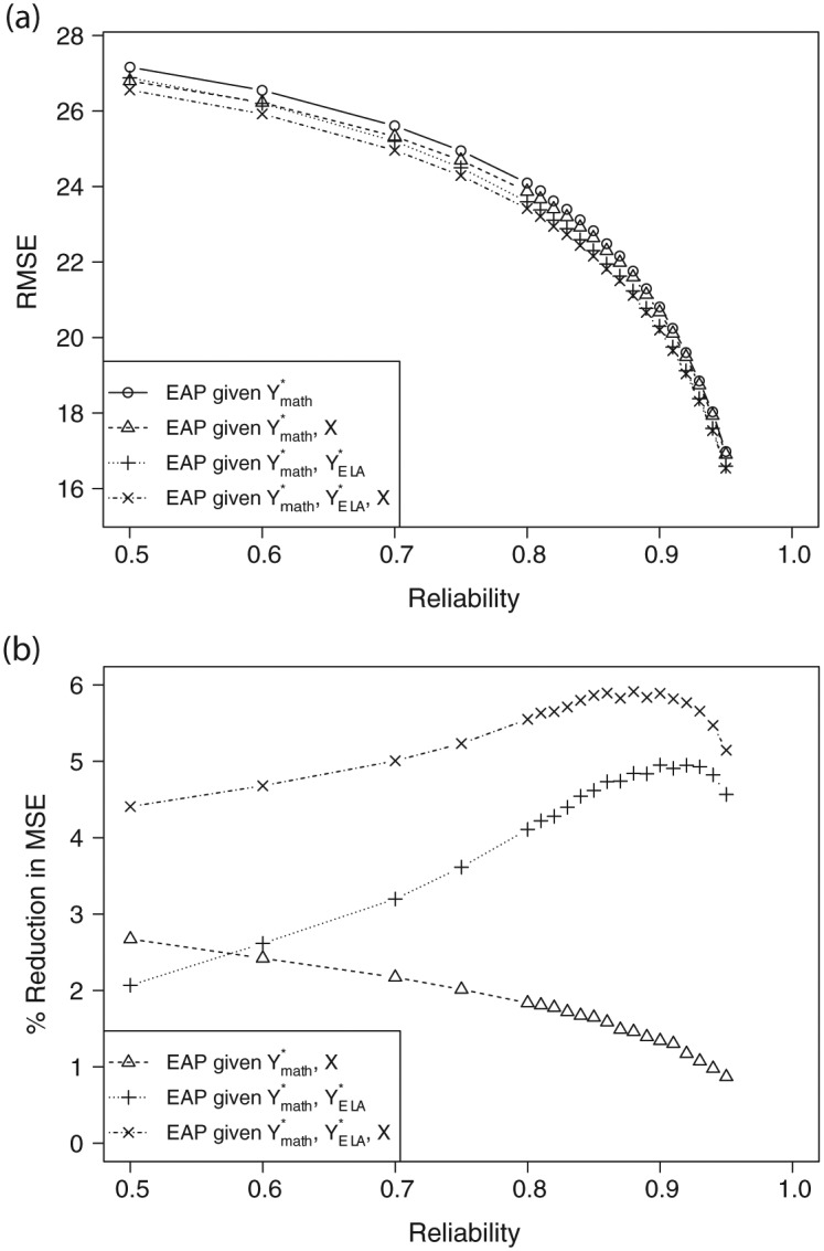
(a) Approximate RMSE of EAP estimators for math SGP conditioning on different amounts of information, as a function of test reliability. (b) Approximate percentage reduction in MSE for different math EAP estimators, relative to the EAP estimator that conditions only on math scores, as functions of test reliability. Values are averaged across Grades 4 to 8.
Figure 1(b) calibrates the improvements in terms of percentage reduction in MSE (Haberman, 2008; Sinharay et al., 2011) relative to the default EAP estimator that conditions only on math scores. Adding covariates alone (curve with triangles) provides only a few percentage point improvement, with benefits increasing as the test reliability decreases. Adding ELA scores alone (curve with +) provides somewhat more benefit, but the relationship is not monotonic with the test reliability. Conditioning on both sources of information (curve with ×) leads to percentage reductions in MSE that are at best 6%. The corresponding maximum for ELA (not shown) is 7%. Curiously, the percentage reduction is maximized with reliability between 0.85 and 0.90, typical values for actual standardized assessments. This means that given the state of the world, the relative benefit provided by conditioning on auxiliary information is about as large as it could be, even though in absolute terms the accuracy gains will not be large.
It is important to clarify that our calculations here hold constant the definition of the true SGP as conditioning on only the matched-subject prior year achievement. For example, the true math SGP is defined as a function of the current and prior year math achievement. This is true even as we consider using both current and prior ELA scores in addition to the math scores to estimate it. This is in contrast to the case where the definition of the true SGP is changed to include additional prior achievement attributes in the conditioning. Monroe and Cai (2015) consider this issue and find that including additional scores in the conditioning set when defining true SGPs tends not to improve estimation accuracy, and actually can decrease it under some circumstances. We consider true SGPs conditioning on multiple prior year scores in the following section as part of our investigation of SGPs aggregated to the teacher level.
Implications for Aggregating SGPs to the Teacher Level
Previous results established that distributions of true SGPs vary as a function of student covariates. Here we consider the implications of this fact for the behavior of aggregates of SGPs to the teacher level, currently used for teacher evaluations (e.g., Colorado Department of Education, 2013; Georgia Department of Education, 2014). Specifically, we use to estimate the expected true SGPs as a function of student covariates . We then use student-teacher links in our data to study the variability across teachers in expected true SGPs based on the characteristics of the students they teach.
Such variation indicates a correlation between the background characteristics of the students a teacher teaches and the average of these students’ true SGPs. The variation results from the combination of the unequal distribution of student covariates across classrooms and the relationships of true SGPs with these covariates. There are at least three distinct mechanisms for these relationships. First, they could result from student-level factors (e.g., motivation, skills, or family circumstances) that are related to both true SGPs and the observed student covariates. Second, they could result from contextual effects, where students have more or less growth as a result of contextual factors (e.g., neighborhoods or classroom dynamics) that are correlated with the observed student covariates. Either of these two mechanisms would pose a problem for interpreting aggregate SGPs as teacher performance indicators because they would cause teachers of equal effectiveness, but who teach different types of students, to receive systematically different aggregate SGPs. The third possible mechanism for relationships of true SGPs with student covariates is the sorting of more or less effective teachers to schools and classrooms that vary systematically with respect to our student background variables. That is, if more effective teachers are more likely to teach students with particular background characteristics, then such students on average may have higher true SGPs simply because they are taught by better teachers. In our investigations of true SGPs aggregated to the teacher level, we conduct some analyses that try to shed light on the contributions of these different mechanisms.
Method
Our analysis of aggregated expected SGPs consisted of four steps. First, for each cohort, we used samples from to compute estimates and of the conditional expectation functions of the true math and ELA SGPs given student covariates. We estimated these functions using linear regressions of and on and again using the smearing method of Duan (1983). The substantive results were not sensitive to alternative modeling decisions to compute the functions, including the expansion of the regression model to include two-way interactions among the covariates, the use of a logit rather than probit function to transform and , and the use of linear regression specifications for and directly.
In the second step, we computed and for each student in the analysis sample for a given cohort. That is, we evaluate the conditional expectation functions estimated from our Monte Carlo samples for each student in the analysis sample, so that each student in that sample is assigned an expected true math SGP and an expected true ELA SGP based on his/her covariates .
In the third step, we restricted the analysis sample for each cohort to students for whom we observed either a math teacher link or an ELA teacher link for Grade . Because part of the appeal of SGPs is their invariance to scale, we then pooled the data across cohorts and both subjects, consistent with common practice in state teacher evaluation systems in which teachers receive a single aggregated “growth” score across all their students (e.g., Georgia Department of Education, 2014). Thus, in the pooled data set, each unique teacher is associated with the expected true math SGPs of the students to whom they teach math, and the expected true ELA SGPs of the students to whom they teach ELA, regardless of those students’ grade levels.
Finally, in the fourth step, we averaged all these expected SGPs to the teacher level for each teacher. If the average for a particular teacher is 60, for example, it indicates that given the background characteristics of the students he or she teaches, we would expect that the teacher would receive an average SGP of 60 (on the 0-100 scale) if there were no measurement error in either the prior or current year tests. We then restricted attention to teachers with 15 or more expected SGPs contributing to the teacher-level mean to mitigate the impact of small samples on the estimated distribution, resulting in 12,103 teachers with “class” sizes ranging from 15 to 221 with a median of 46. For middle school teachers who tend to teach either math or ELA but not both, the restriction generally means that teachers needed to be linked to at least 15 students. For elementary school teachers who teach both subjects, the number of actual students might be as small as 8 because each student contributes both a math and ELA expected SGP.
Results
Figure 2 provides a histogram of the teacher-level averages of the expected true SGPs for the sample of teachers described above. The distribution has some low outliers below 40, and a heavier right tail that extends above 60. The 0.10 and 0.90 quantiles are 44.8 and 55.4, respectively. Other authors have noted that SGPs estimated from test scores and then aggregated to the teacher level can be correlated with aggregated student background characteristics solely as a result of measurement error in the prior test scores used to estimate SGPs (McCaffrey et al., 2015; Shang et al., 2015). Our results go further: they indicate that such relationships would exist even if true SGPs could be measured perfectly through tests with no measurement error.
Figure 2.

Histogram of estimated expected true SGP at the teacher level based on student covariates for teachers with at least 15 expected SGPs.
The variability of the distribution is striking, but as noted in the previous section, there are multiple mechanisms that could be responsible for the correlation between true SGPs and student covariates that ultimately leads to the type of variability evident in Figure 2 when teachers vary with respect to the types of students they teach. We conducted several analyses that probed these mechanisms. First, we investigated whether we obtained distributions similar to Figure 2 if we considered expected SGPs given lag-1 prior achievement in the other subject or given additional years of prior achievement from the same subject. Conditioning on additional prior achievement attributes is a common strategy for matching students more closely with respect to prior achievement (Lockwood & McCaffrey, 2014), potentially reducing the magnitude of relationships between other student covariates and student progress. That is, if part of the relationship between true SGPs and observed student covariates is due to unobserved student-level factors correlated with both, then conditioning on additional information that may proxy for such factors can help to reduce the correlation between true SGPs and observed student covariates.
We can easily obtain true SGP distributions for, say, current math achievement given both prior math and ELA achievement using the models presented to this point. For true SGPs given additional lagged prior achievement, we ran additional latent regression models where the four dimensions were 4 years of achievement for a single subject (e.g., math achievement in Grades 3 [2007] to 6 [2010]), which allowed us to examine distributional properties of true SGPs conditional on up to 3 years of prior achievement. In summary, using these true SGP distributions and the methods described above for obtaining average expected SGPs for teachers given student background covariates, we found only a modest reduction in variance. Specifically, versions of the distribution in Figure 2 based on including additional prior achievement attributes would have a standard deviation ranging from 78% to 85% as large as that of the distribution in Figure 2. Thus, the large spread evident in Figure 2 is not removed simply by conditioning on more prior achievement traits.
We also conducted analyses that tried to isolate the part of the observed relationships between expected SGPs and student covariates that are due only to individual-level relationships. These analyses are described in the appendix. The results are summarized in Figure 3, which is analogous to Figure 2 but is based on only individual-level relationships between background characteristics and true SGPs, and does not reflect variation due to either contextual effects or sorting of teachers of different effectiveness to different types of students. The standard deviation of the distribution in Figure 3 is 63% as large as that of the distribution in Figure 2. In addition, spread between the 0.10 and 0.90 quantiles in Figure 3 is (46.9, 53.5), compared with (44.8, 55.4) for Figure 2. Thus, our analyses suggest that even if part of the spread in Figure 2 is due to contextual effects or teacher sorting, variation across teachers in expected aggregated SGP would remain due to individual student-level relationships and variation across teachers in the types of students they teach.
Figure 3.

Histogram analogous to Figure 2, but based on within-group latent regression coefficients.
Discussion
Studying properties of true SGPs only through the lens of estimated SGPs is difficult due to excessive estimation error in estimated SGPs. Modeling longitudinal item-level data with latent regression MIRT models is an efficient and effective alternative. The latent regression specification leads directly to model-based true SGP functions, and the parameters required to specify these functions can be estimated straightforwardly in the MIRT framework. Monte Carlo methods can then be used to study features of the joint distribution of multiple true SGPs, student covariates, and test scores that, to date, have not been investigated.
Our results raise concerns about using and interpreting estimated SGPs at both the student and aggregate levels. A substantial research base already notes that SGP estimates for individual students have large errors (Lockwood & Castellano, 2015; McCaffrey et al., 2015; Monroe & Cai, 2015; Shang et al., 2015). Our findings indicate that joint models capitalizing on relationships of true SGPs both across subjects and with student covariates would provide only modest benefits for estimation accuracy. Although this accuracy problem manifests with SGPs, it is not unique to SGPs: it is an intrinsic problem with trying to use typical standardized assessments to measure growth accurately (Harris, 1963). Our findings underscore that using multiple features of the observed data to learn about true growth cannot overcome this fundamental limitation. Thus, estimated SGPs may not be accurate enough to support inferences or decision making for individual students.
The fact that SGPs apparently are related to student background characteristics even in the absence of test measurement error, with directions of the relationships generally echoing those observed with achievement status, creates further interpretation problems. On the one hand, our finding that excessive absence is a strong predictor of true SGPs provides some reassurance that tests can be sensitive to time-varying factors that we would hope to have causal impacts on student progress. On the other hand, relationships with persistent characteristics such as race/ethnicity suggest that the process of conditioning on prior achievement, even if it could be measured accurately, will result in achievement progress measures that carry with them some part of the gaps seen with achievement status. This creates a dissonance between some of the rhetoric surrounding the fairness of growth measures such as SGPs, and the reality of how such measures are likely to behave. Our finding that these relationships exist with latent achievement attributes, not just with observed test scores, makes clear that improving the reliability of standardized assessments would be insufficient to solve this problem.
The relationships of true SGPs to student characteristics also creates a clear problem for interpreting estimated SGPs aggregated to the teacher or school levels. One of the putative benefits of aggregating estimated SGPs is that it overcomes the excessive measurement error problem at the individual level. However, the variability in the distribution in Figure 2 is troubling, and our evidence that a nontrivial part of that variability may be due to individual-level relationships between student characteristics and true SGPs is even more troubling. It suggests that SGPs aggregated to the teacher level may contain a source of variance that is due solely to the fact that teachers do not teach the same types of students. This source of variance represents bias if the goal is to interpret aggregated SGP as an indicator of teacher effectiveness. This bias is easy to avoid in a value-added model that regresses student test scores on teacher fixed effects, prior test scores, and student background variables because such a model removes variance due to the individual-level relationships from the estimated teacher effects (see, e.g., Wooldridge, 2002). Our results thus suggest that the interpretation and transparency benefits provided by aggregated SGPs need to be weighed against the costs of allowing a source of bias in performance indicators that is removed by alternative modeling approaches.
Our results come with a number of caveats. The main limitation results from the specification of the latent regression model in Equation 1. Although such a specification is standard in MIRT modeling, and is useful for analyzing aspects of the statistical structure of achievement attributes and their relationships to student characteristics, it falls short of being a structural (causal) model for the evolution of student achievement. Such models specify student achievement as a cumulative function of the history of educational inputs (e.g., teacher and school effects), peer effects, and effects of both observed and unobserved individual and family attributes (see, e.g., Todd & Wolpin, 2003). Provided the many assumptions required to estimate such models with real data are appropriate, they have the advantage that they permit the sorts of decompositions needed to fully interpret, for example, the distribution in Figure 2 because they disentangle the causal effects of various inputs to student achievement. We have no reason to think that our second-stage analyses probing the decomposition provide misleading results. However, more refined inferences would be possible if the latent regression part of the MIRT model was specified as something closer to a structural model for longitudinal student achievement. Such modeling introduces a number of challenges, including data requirements, model specification decisions (e.g., how to deal with the cross-classification of students to teachers over time as well as missing student-teacher links), and software limitations that are beyond the scope of this article. Future work along these lines could build on our framework under more complex model specifications.
Other modeling decisions may have affected our results. For example, our latent regression included only main effects for the covariates. Preliminary analyses with the scale scores suggested some evidence for two-way interactions, but the increase in R2 for such model terms was 0.01 or less, and including them in the MIRT models would have substantially increased computation time and complicated interpretation of the model parameters. It is unlikely that accounting for these interactions would change any of the substantive findings, but it still may be useful to consider the sensitivity of our findings to such model specification changes. Similarly, our choice of item response model could affect our results, warranting additional analyses to determine the extent that a different model, such as the three-parameter-logistic model for dichotomously scored items, fits the data better and changes our findings, if at all. Finally, it is unlikely that the assumption that the latent trait residuals are independent with a multivariate normal distribution with a constant variance-covariance matrix holds exactly. There is no reason to think that the misspecification of the model is so severe that fitting a more authentic model would lead to drastic changes in the findings, but it would be useful to relax these assumptions and investigate the extent to which our findings are robust.
Some of our findings also may be due to peculiarities of our data set. For instance, in preliminary analyses, we found that student background covariates still had relatively large coefficients when included in a regression of current year (2010) scores on several prior year scores. Thus, for our data, student background covariates seem to explain additional variation in current test scores over and above prior achievement. This may not be typical, which could contribute to the several large group differences in true SGPs we find.
Finally, the inferences from our EAP analyses may also be sensitive to several choices we made beyond those made in the latent regression MIRT model. For example, we approximated EAPs under the assumption of homoscedastic measurement error, which does not generally hold with IRT-based ability estimates based on linear test forms. We suspect that our substantive conclusions are not sensitive to allowing for heteroskedastic error but future research may consider to what extent it does matter. It may lead to shrinkage being more important for students in the tails of the test score distributions because their test scores are typically noisier.
Although such future research would be useful to investigate the robustness of our findings, this study serves as an important step in investigating the properties of the underlying quantities attempting to be measured by SGPs computed from error-prone test scores, and the implications of those properties for the validity of SGPs as indicators of student achievement growth and educator effectiveness.
Supplementary Material
Acknowledgments
We thank Shelby Haberman, Daniel F. McCaffrey, Peter van Rijn, the editor, and two referees for providing constructive comments on earlier drafts.
Appendix
Details on True SGP Computation
Equation 2 is straightforward to evaluate when and are known. The term requires only the evaluation of a univariate normal CDF with mean and variance determined by , , and using standard formulas for conditional distributions from multivariate normal variables (see, e.g., Anderson, 1984). The second term covers the case where is discrete or continuous. In our application, all covariates are discrete and so is discrete. In this case, Equation 2 reduces to
where are the possible values of with probabilities . For instance, for the data from our Grade 4 cohort, there are H = 1,630 distinct groups defined by the observed unique combinations of the student covariates used in our model. The terms are straightforward to evaluate using Bayes rule. They are obtained by multiplying the prior probabilities by , and then normalizing the products so that they sum to one over h = 1, . . . , H. Each term is simply a (possibly multivariate) normal density with parameters determined by , , and .
Assessing Uncertainty
We conducted the following analyses to assess how much uncertainty there is in various inferences reported in the article due to the three sources of uncertainty noted in the “Estimating Latent Regression Models and True SGP Distributions” section. To keep computations manageable, we focused on the Grade 7 cohort. This cohort has the smallest sample size (N = 65,093) among the five cohorts and so should have the most estimation error; however, the cohort sizes are extremely similar and so it reasonable to assume that what is learned from the Grade 7 cohort regarding uncertainty would generalize to all cohorts. We drew J = 10 bootstrap samples from the Grade 7 cohort (Efron & Tibshirani, 1993) and estimated the MIRT model for each. This resulted in estimated parameters for each of the j = 1, . . . , 10 bootstrap samples. Variability among these estimates reflects both sampling variability due to the sample of students and Monte Carlo variability in the MH-RM solutions. The total variability was small. The average bootstrap standard error for the regression coefficients was 0.023, with an average absolute magnitude of the coefficients themselves of 0.36. The average bootstrap standard error for the R2 of the covariates in the latent regressions for the Grade 7 cohort was only 0.003. Likewise, the average bootstrap standard error for the correlation parameters was only 0.0025. Thus, the resulting 95% confidence intervals for these quantities are sufficiently narrow to not affect the substantive conclusions.
The inferences regarding true SGPs have additional uncertainty due to the Monte Carlo samples used to compute them. For each j, we independently drew B = 1,000,000 samples from where was based on and , the empirical distribution of the covariates in bootstrap sample j. Thus, these samples reflect all three sources of uncertainty. The bootstrap standard error for the correlation between the true math and ELA SGPs was 0.008. The average bootstrap standard error for the mean differences in true SGP by covariate group was 0.41 (on the 0-100 SGP scale).
Auxiliary Analysis to Investigate Possible Sorting Bias
Our goal was to investigate how much of the variation in Figure 2 might be due to individual-level relationships of student covariates to SGPs, rather than due to either contextual effects or relationships of true teacher effectiveness to student background characteristics (i.e., systematic teacher sorting). The MIRT model in Equation 1 does not decompose covariate effects into within-teacher and between-teacher components. We thus conducted analyses that used such a decomposition to isolate the within-teacher latent regression coefficients and created a version of Figure 2 where expected true SGPs were based only on these coefficients rather than the marginal coefficients.
Our analyses proceeded as follows. For each cohort, we began with the analysis samples used for the main MIRT models and summarized in Table 1. For each of the four dimensions in a cohort, we merged teacher links onto the data for the corresponding grade level and subject. For example, for dimension k = 1, we merged ELA teacher links for Grade g – 1, whereas for dimension k = 4, we merged math teacher links for Grade g. We then restricted the data for each dimension to records from students linked to teachers with at least 10 students. For this restricted sample, and for each model covariate, we computed both the teacher-level mean and the deviation from the teacher-level mean. Thus, for each dimension, the original vector of covariates for each student is replaced with the vector , where is the vector of teacher-level mean covariates for teacher j and j(i) is the index j of the teacher to whom student i is linked for the appropriate grade and subject. We then fit a one-dimensional latent regression IRT model to the data from each dimension and recovered the coefficients on the within-teacher deviations , which we denote by to indicate that these are the coefficients on the within-teacher deviations for dimension k. We then let . These coefficients are unaffected by either contextual effects or teacher sorting since both teacher and context are assumed to be constant among students sharing a teacher. In this sense, they reflect only the individual-level relationships between latent achievement traits and student background variables. We used separate one-dimensional models rather than a single four-dimensional model to avoid collinearity and sample restriction issues that arose when fitting the four-dimensional model with the augmented covariates due to the cross-classification of students to teachers both across subjects and across grades.
We then replicated the calculations that led up to Figure 2, but when we generated samples from the latent regression model, we used rather than . Thus, the latent achievement traits are simulated from a distribution where their relationships to the covariates are based only on within-teacher relationships rather than the marginal relationships. All remaining computations proceeded as before. The resulting distribution of expected true SGPs aggregated to the teacher level is given in Figure 3. The 0.05, 0.10, 0.25, 0.50, 0.75, 0.90, and 0.95 quantiles of this distribution are 46.2, 46.9, 48.2, 49.6, 51.5, 53.5, and 54.9. The corresponding values from the distribution in Figure 2 are 43.5, 44.8, 46.7, 49.1, 52.6, 55.4, and 56.9. The distribution is thus more concentrated when is used. However, there is still substantial variability among teachers in this distribution. The SD of the distribution using is 63% as large as the SD of the distribution in Figure 2, as reported in the text.
Note that our model of interest is distinct from IRT growth curve models that rely on common items across time points and model change in achievement over time. SGPs do not model absolute change in achievement over time. Rather, they are a normative measure of growth, or as Castellano and Ho (2013) describe them, measures of “conditional status” in that they describe a student’s current status relative to students with the same prior status.
We also ran all latent regression models with Haberman’s (2015) mirt software that uses adaptive quadrature and obtained essentially identical parameter estimates. Details are available on request.
Authors’ Note: The opinions expressed are those of the authors and do not represent views of the Institute of Education Sciences or the U.S. Department of Education.
Declaration of Conflicting Interests: The author(s) declared no potential conflicts of interest with respect to the research, authorship, and/or publication of this article.
Funding: The author(s) disclosed receipt of the following financial support for the research, authorship, and/or publication of this article: This material was supported in part by the Institute of Education Sciences, U.S. Department of Education, through Grant R305D140032 to ETS.
Supplemental Material: Supplemental material for this article is available online.
References
- Adams R., Wilson M., Wang W. (1997). The multidimensional random coefficients multinomial logit model. Applied Psychological Measurement, 21, 1-23. [Google Scholar]
- Akram K., Erickson F., Meyer R. (2013). Issues in the estimation of student growth percentiles. Paper presented at the annual meeting of the Association for Education Finance and Policy, New Orleans, LA. [Google Scholar]
- Anderson T. (1984). An introduction to multivariate statistical analysis (2nd ed.). New York, NY: Wiley. [Google Scholar]
- Betebenner D. (2009). Norm- and criterion-referenced student growth. Educational Measurement: Issues and Practice, 28(4), 42-51. [Google Scholar]
- Billingsley P. (1995). Probability and measure (3rd ed.). New York, NY: Wiley. [Google Scholar]
- Briggs D., Betebenner D. (2009). Is growth in student achievement scale dependent? Paper presented at the annual meeting of the National Council for Measurement in Education, San Diego, CA. [Google Scholar]
- Cai L. (2010). Metropolis-Hastings Robbins-Monro algorithm for confirmatory item factor analysis. Journal of Educational and Behavioral Statistics, 35, 307-335. [Google Scholar]
- Casella G., Berger R. L. (1990). Statistical inference. Belmont, CA: Duxbury Press. [Google Scholar]
- Castellano K. E., Ho A. D. (2013). Contrasting OLS and quantile regression approaches to student “growth” percentiles. Journal of Educational and Behavioral Statistics, 38, 190-215. [Google Scholar]
- Chalmers R. P. (2012). mirt: A multidimensional item response theory package for the R environment. Journal of Statistical Software, 48(6), 1-29. [Google Scholar]
- Colorado Department of Education. (2013). Measures of student learning guidance for districts: Version 2.0. Retrieved from http://www.cde.state.co.us/sites/default/files/MeasuresofStudentLearningFINAL081413.pdf
- de la Torre J. (2009). Improving the quality of ability estimates through multidimensional scoring and incorporation of ancillary variables. Applied Psychological Measurement, 33, 465-485. [Google Scholar]
- Duan N. (1983). Smearing estimate: A nonparametric retransformation method. Journal of the American Statistical Association, 78, 605-610. [Google Scholar]
- Efron B., Morris C. (1973). Stein’s estimation rule and its competitors: An empirical Bayes approach. Journal of the American Statistical Association, 68, 117-130. [Google Scholar]
- Efron B., Tibshirani R. (1993). An introduction to the bootstrap. New York, NY: Chapman & Hall. [Google Scholar]
- Georgia Department of Education. (2014). Leader keys effectiveness system: Implementation handbook. Retrieved from https://www.gadoe.org/School-Improvement/Teacher-and-Leader-Effectiveness/Documents/FY15%20TKES%20and%20LKES%20Documents/LKES%20Handbook-%20%20FINAL%205-30-14.pdf
- Haberman S. J. (2008). When can subscores have value? Journal of Educational and Behavioral Statistics, 33, 204-229. [Google Scholar]
- Haberman S. J. (2015). A general program for item-response analysis that employs the stabilized Newton-Raphson algorithm. Princeton, NJ: ETS. [Google Scholar]
- Harris C. (1963). Problems in measuring change. Madison: University of Wisconsin Press. [Google Scholar]
- Lockwood J. R., Castellano K. E. (2015). Alternative statistical frameworks for student growth percentile estimation. Statistics and Public Policy, 2(1), 1-8. [Google Scholar]
- Lockwood J. R., McCaffrey D. F. (2014). Correcting for test score measurement error in ANCOVA models for estimating treatment effects. Journal of Educational and Behavioral Statistics, 39(1), 22-52. [Google Scholar]
- Lord F. (1980). Applications of item response theory to practical testing problems. Hillsdale, NJ: Erlbaum. [Google Scholar]
- McCaffrey D. F., Castellano K. E., Lockwood J. R. (2015). The impact of measurement error on the accuracy of individual and aggregate SGP. Educational Measurement: Issues and Practice, 34(1), 15-21. [Google Scholar]
- Mislevy R., Beaton A., Kaplan B., Sheehan K. (1992). Estimating population characteristics from sparse matrix samples of item responses. Journal of Educational Measurement, 29, 133-161. [Google Scholar]
- Mislevy R., Johnson E., Muraki E. (1992). Scaling procedures in NAEP. Journal of Educational Statistics, 17, 131-154. [Google Scholar]
- Monroe S., Cai L. (2015). Examining the reliability of student growth percentiles using multidimensional IRT. Educational Measurement: Issues and Practice, 34(4), 21-30. [Google Scholar]
- Muraki E. (1992). A generalized partial credit model: Application of an EM algorithm. Applied Psychological Measurement, 16, 159-176. [Google Scholar]
- R Core Team. (2015). R: A language and environment for statistical computing. Vienna, Austria. Retrieved from http://www.R-project.org/
- Shang Y., Van Iwaarden A., Betebenner D. (2015). Covariate measurement error correction for student growth percentiles using the SIMEX method. Educational Measurement: Issues and Practice, 34(1), 4-14. [Google Scholar]
- Sinharay S., Puhan G., Haberman S. J. (2011). An NCME instructional module on subscores. Educational Measurement: Issues and Practice, 30(3), 29-40. [Google Scholar]
- Todd P., Wolpin K. (2003, February). On the specification and estimation of the production function for cognitive achievement. Economic Journal, 11, F3-F33. [Google Scholar]
- von Davier M., Sinharay S. (2010). Stochastic approximation methods for latent regression item response models. Journal of Educational and Behavioral Statistics, 35, 174-193. [Google Scholar]
- Wooldridge J. (2002). Econometric analysis of cross section and panel data. Cambridge: MIT Press. [Google Scholar]
Associated Data
This section collects any data citations, data availability statements, or supplementary materials included in this article.