Automatic localization of three-dimensional cephalometric landmarks on CBCT images by extracting symmetry features of the skull

Abstract

To propose an algorithm for automatic localization of 3D cephalometric landmarks on CBCT data, those are useful for both cephalometric and upper airway volumetric analysis. 20 landmarks were targeted for automatic detection, of which 12 landmarks exist on the mid-sagittal plane. Automatic detection of mid-sagittal plane from the volume is a challenging task. Mid-sagittal plane is detected by extraction of statistical parameters of the symmetrical features of the skull. The mid-sagittal plane is partitioned into four quadrants based on the boundary definitions extracted from the human anatomy. Template matching algorithm is applied on the mid-sagittal plane to identify the region of interest ROI, further the edge features are extracted, to form contours in the individual regions. The landmarks are automatically localized by using the extracted knowledge of anatomical definitions of the landmarks. The overall mean error for detection of 20 landmarks was 1.88 mm with a standard deviation of 1.10 mm. The cephalometric land marks on CBCT data were detected automatically with in the mean error less than 2 mm.

Introduction

Cephalometric analysis plays a vital role in orthodontic diagnosis and treatment planning. Conventionally, cephalometric analysis is performed using 2D radiographs. Automation incephalometric landmark identification is a plus for computer aided diagnostics (CAD). It can be observed that there is a plethora of scientific literature on algorithms for 2D cephalometric landmark identification on X-ray radiographs.^{1, 2} There are several limitations in conventional 2D radiographs such as nonlinear magnification, distortion, projected measurements and overlapping of craniofacial structures^{3, 4} etc. Though, with technological progress and evolution of cone-beam computed tomography (CBCT), limitations associated with 2D conventional radiographs have been overcome. Few studies, offered a stimulating insight into automated 3D cephalometric landmark detection algorithm development.^–

Pan Zheng et al¹⁰ had shown a method for visualization of craniofacial structures and landmarks using visualization toolkit and wrapper language. A program for identification and manipulation of landmark on hard tissue of digitized craniofacial data was generated. The discussed method was not fully automatic. Makram et al¹³ had proposed automatic landmark localization on CBCT image using reeb graph nodes. 18 of the targeted 20 landmarks were successfully identified using reeb graph nodes approach and hence, reported a 90% success rate. This algorithm was applied only on one CBCT image; hence, the statistical confidence is questionable to conclude the clinical significance. Cheng et al⁵ proposed a discriminative method for automatic detection of single landmark from CBCT dental volumes. Random forests algorithm combined with sampled context features were used in the approach. In order to increase the efficiency, constrained search process was integrated with a special prior. The algorithm has been implemented to detect only one landmark. Keustermans et al⁷ proposed a statistical model-based approach for automatic localization of cephalometric landmarks on CBCT using shape and local appearance models. Usage of both local and global shape models along with the definitions of edges between the landmarks is arbitrary. Unified approach, multiscale scheme helps in improving the results. Keustermans et al⁸ in 2011 again came up with statistical model-based approach by incorporating both sparse appearance and shape models. This is an energy optimization-based approach, multilabel Markov Random Fields have been used for optimization of the energy obtained through maximum posteriori approach. The robustness of the algorithm was tested on 37 CBCT data sets of patients undergoing maxillofacial surgery. Shahidi et al⁹ had proposed a feature-based and voxel similarity-based registration algorithm for identification of craniofacial landmarks using CBCT data. Registration-based approach is further prone to errors for patients presenting with different kinds of deformities, e.g. levels of malocclusion. This restraint also limited the exploitation of algorithm towards clinical 3D cephalometric analysis. Codari et al¹¹ had proposed an intensity-based registration approach for automatic estimation of cephalometric landmarks on the skull. The major limitation of this algorithm was requirement of different atlases for different category of patients with different sex, age and ethnicity. The algorithm provided acceptable results for only one class of patients for which the atlases were priory prepared. Gupta et al^{6, 12} had proposed a knowledge-based approach for landmark detection on CBCT images. This algorithm used template matching approach for detection of seed point. Volume of interest (VOI) was calculated by using distance vector from the empirical point. The respective contours were detected in VOI and then landmarks were localized based on the definitions of the landmarks on the anatomical contours. While the algorithm achieved significantly better results than the previous work and had detected landmarks in bilateral planes, still the robustness of the algorithm towards deformed cases was limited because of the rigid rules in defining the region boundaries for VOI identification. Keeping in view of the said limitations in the existing literature, we have proposed a method for automatic detection of cephalometric landmarks on 3D CBCT image data based on the symmetry features of the skull, dynamic extraction of VOI using spatial information, anatomical boundary definitions and template matching.

Methods and Materials

30 CBCT data sets were collected retrospectively from the archived database of the post-graduate orthodontic clinical database irrespective of age, gender and ethnicity. All scans were obtained using iCAT Next Generation CBCT unit (Imaging Sciences International, Hatfield, PA) with a FOV of 17 × 23 cm and scan time of 26 s. Acquired data sets had images saved in Digital Imaging and Communications in Medicine (DICOM v. 1.7) format with isometric voxel size of 0.25–0.40 mm. Each CBCT data set was imported into Dolphin 3D software (Dolphin Imaging & Management Systems, Chatsworth, CA) and developed into a volume rendered image for reorientation. Transorbitale line in frontal view and Frankfort horizontal line in lateral view were horizontally aligned in each data set. Also, orientation was reconfirmed in top and bottom views by visualizing it symmetrically. After reorientation, new DICOM files were generated for each patient. Thus, data sets were reoriented and standardized for manual landmark plotting as well as automatic detection using the proposed method.

Ground truth generation

To generate the ground truth, targeted landmarks were manually marked by the three experienced orthodontists using MIMICS software (Materialise, Leuven, Belgium). Among the three observers, two had a clinical and research experience of 8 years and another had of 5 years. These three orthodontists underwent training session on the manual landmark plotting using the 3D tool MIMICS. Interobserver reliability was measured between the three observers and found to be >0.98. After confirming good correlation between the observers, the ground truth was generated by calculating the mean co-ordinates of the observers. Reorientation of collected data, and ground truth generation for algorithm validation has been referred from Gupta et al.^{6, 14}

Automatic landmark detection

The algorithm for automatic landmark detection on 3D CBCT data was implemented in MATLAB (MathWorks, Inc.) programming environment. 20 landmarks were targeted for automatic detection. The definitions of these landmarks were taken from the literature^{6, 12,14,15} (as listed in Appendix A). Figure 1 shows the steps involved in the algorithm. An algorithm based on the boundary definitions of the human anatomy for detection of landmarks on CBCT data is presented. Mid-sagittal plane was detected through extraction of statistical parameters from the symmetrical features of the skull. Mid-sagittal plane is a 2D image of sagittal view. Automatic detection of landmarks on mid-sagittal plane requires automatic identification of local region of interests. Template matching approach was used to identify the region of interest and the initial reference landmark—posterior nasal spine (PNS) to initiate the algorithm for quadrant identification and further landmark identification. Using the boundary definitions, mid-sagittal plane was divided into four quadrants and the curves in the individual quadrant were traced automatically through extraction of anterior points in the first and fourth quadrant, superior points in the second quadrant and disconnected components in the third quadrant. Based on the anatomical definitions of the landmarks, they were automatically detected through extraction of geometrical features, e.g. peak, valley, corners and shortest radial distance on the traced curves. The details of the algorithm are explained in Appendix B.

Figure 1.

Methodology for automatic landmark localization using CBCT. VOI, volume of interest.

Results

The landmarks detected automatically for 30 CBCT images were compared with the manually identified landmarks by the three observers on the same data set. The interclass correlation for all the landmarks was found to be greater than 0.9, which gives an evidence for an excellent co-ordination among the three observers. The error for each landmark was calculated by finding the Euclidean distances between the co-ordinates of landmarks obtained through manual identification and automatic detection.

The mean error for all the landmarks except Gonion, Condylion, R1 and Sella were found to be less than 2 mm using the proposed algorithm. C4ai landmark was available only on 25 data sets. Hence, the results were evaluated on 25 data sets. The proposed algorithm has been compared with the knowledge-based algorithm.^{6, 12} Table 1 illustrates a comparison of the mean error, standard deviation (SD) and the percentage rate of detection (success detection) within 2, 3 and 4 mm range of the proposed algorithm and knowledge-based algorithm with the manual approach. The overall average percentage rate of detection of the landmarks through the proposed algorithm within 2, 3 and 4 were found to be 63.53, 85.29 and 93.92%, respectively. The mean error for 14 landmarks was found to be less than 2 mm. Gonion, Condylion (bilateral), R1_R and Sella were the landmarks having mean error greater than 2 mm. Five landmarks [Nasion, anterior nasal spine (ANS), PNS, R1_L and Menton) were detected within 4 mm error range of manual landmarking for all the 30 CBCT images, i.e. 100%.

Table 1.

Mean error and SD for landmark detection and percentage rate of detection less than 2, 3 and 4 mm error with comparison to knowledge-based approach^{6, 12}

Land marks	Mean ± SD		Percentage rate of landmark detection
Knowledge- based	Proposed method	Knowledge- based	Proposed method	Knowledge- based	Proposed method	Knowledge-based	Proposed method
<2 mm	<2 mm	<3 mm	<3 mm	<4 mm	<4 mm
N	1.17 ± 0.49	0.95 ± 0.69	93.33	90.00	100.00	100.00	100.00	100.00
A-Pt	1.73 ± 0.80	1.91 ± 0.94	76.67	50.00	93.33	90.00	96.67	96.67
ANS	1.42 ± 0.73	1.03 ± 0.62	73.00	93.33	80.00	96.67	96.67	100.00
PNS	2.08 ± 1.29	1.60 ± 1.15	56.67	76.67	76.67	93.33	93.33	100.00
B-Pt	2.08 ± 1.09	1.78 ± 0.91	53.33	63.33	80.00	93.33	93.33	96.67
Po	1.53 ± 0.79	1.77 ± 0.96	80.00	70.00	96.67	86.67	96.67	96.67
Me	1.21 ± 0.58	1.57 ± 0.54	90.00	70.00	100.00	100.00	100.00	100.00
Gn	1.62 ± 0.62	1.64 ± 0.68	76.67	66.67	93.33	83.33	100.00	86.67
GoL	2.04 ± 1.47	2.02 ± 1.09	63.33	56.67	76.67	76.67	86.67	96.67
GoR	2.47 ± 1.37	2.10 ± 1.18	46.67	50.00	66.67	80.00	83.33	90.00
CoL	3.20 ± 2.49	3.78 ± 2.77	36.67	26.67	60.00	50.00	70.00	70.00
CoR	2.38 ± 1.71	3.34 ± 2.47	53.33	33.33	70.00	70.00	83.33	83.33
R1L	2.05 ± 1.22	1.40 ± 0.81	56.67	80.00	86.67	93.33	90.00	100.00
R1R	2.26 ± 1.07	2.10 ± 1.12	60.00	60.00	80.00	73.33	86.67	93.33
ZyL	2.80 ± 1.63	1.74 ± 1.01	36.67	70.00	53.33	90.00	76.67	93.33
ZyR	2.83 ± 2.05	1.48 ± 1.05	46.67	73.33	70.00	93.33	70.00	96.67
Sella	1.52 ± 0.75	2.19 ± 0.91	70.00	50.00	96.67	80.00	100.00	96.67
C2sp	NA	1.59 ± 0.92	NA	73.33	NA	93.33	NA	93.33
C3ai	NA	1.70 ± 1.05	NA	70.00	NA	86.67	NA	90.00
C4ai	NA	1.95 ± 1.25	NA	60.00	NA	88.00	NA	92.00

ANS, anterior nasal spine; NA, not available; PNS, posterior nasal spine; SD, standard deviation.

Discussion

An algorithm for automatic detection of 20 landmarks has been developed for 3D CBCT images data. The proposed algorithm was compared with the recent state of the art method knowledge-based approach for automatic landmark detection.^{6, 12} 17 landmarks are in common for both the approaches, while, 3 landmarks in the cervical vertebrae region were additionally detected in our approach, which are useful in upper airway analysis on 3D volumetric data. Landmarks Nasion, ANS, PNS, B-point, Gonion left, Gonion right, R1 (left and right) and Zygomatic (left and right) have shown relatively less mean error compared with the knowledge-based approach and thus, were detected with higher accuracy. Seven landmarks A-point, Pogonion, Gnathion, Menton, Sella and Condylion (left & right) have shown higher mean differences when compared with the knowledge-based approach.

The success detection rate was calculated within the range of 2, 3 and 4 mm of manual identification. The successful detection rate within 2, 3 and 4 mm error range of manual marking was compared with the knowledge-based approach for all the 17 common landmarks. Seven landmarks (ANS, PNS, B-pt, Go_R, R1_L, Zy_L, Zy_R) have shown better detection rate and one landmark (R1_R) has shown equal detection rate within 2 and 3 mm range, whereas nine landmarks (ANS, PNS, B-pt, Go_L, Go_R, R1_L, R1_R, Zy_L, Zy_R) have shown better detection rate and six landmarks (N, A-pt, Pog, Me, Co_L, Co_R) have shown equal detection rate within 4 mm error range. In knowledge-based approach the values chosen for the distance vector to VOI identification are static, based on rigid definitions. Hence, the robustness is the major challenge in the knowledge-based approach with severely deformed cases. Algorithm may fail because of the rigid adoption. Proposed algorithm is based on the knowledge derived from the human anatomy. The knowledge is provided by selecting the boundary definitions based on the human anatomy. No static inputs have to be provided as a prior knowledge for VOI extraction. Hence, the aforementioned limitation can be circumvented while achieving better or an equal accuracy and reliability. The proposed algorithm has shown improved detection rate in all the three ranges, i.e. 2 mm (63.53%), 3 mm (85.29%) and 4  mm (93.92%) in comparison to knowledge-based approach. Mean error (1.91 mm) and SD (1.11 mm) for all the 17 landmarks have improved when compared with the knowledge-based approach.

Conclusions

An algorithm based on the boundary definition of the human anatomy for automatic detection of landmarks on 3D CBCT image is presented. The algorithm was tested on 30 CBCT images and found an overall mean error of 1.88 mm and SD of 1.10 mm for 20 landmarks. The overall detection rate was recorded as 64.16, 85.89 and 93.60% within 2, 3 and 4 mm range, respectively, which is an improved result from the available state-of-the-art techniques. The robustness of the algorithm has to be further tested on severely deformed cases and on a few cases with different races and ethnicity.

Appendix A

S. no	Landmark	Abbreviation	Definition on skull
1.	Nasion	N	Most anterior point of the frontonasal suture in the mid-sagittal plane
2.	A-point hard	A-point	The point at the deepest midline concavity on the maxilla between the anterior nasal spine and the dental alveolus
3.	Anterior nasal spine	ANS	Most anterior midpoint of the ANS of maxilla
4.	Posterior nasal spine	PNS	The sharp posterior extremity of the nasal crest of the hard palate
5.	B-point hard	B-point	Most posterior point in the concavity along the anterior border of the mandibular symphysis
6.	Pogonion hard	Pog/Pg	Most anterior point on mandibular symphysis
7.	Menton hard	Me	Most inferior point on the mandibular symphysis
8.	Gnathion hard	Gn	Midpoint of the curvature of the pogonion and menton
9.	Gonion left	GoL	Most inferior and posterior point on left mandibular corpus
10.	Gonion right	GoR	Most inferior and posterior point on right mandibular corpus
11.	Condylion left	CoL	Most superior point on the left mandibular condyle
12.	Condylion right	CoR	Most superior point on the right mandibular condyle
13.	R1 left	R1L	The deepest point on the curve of the anterior border of the left ramus
14.	R1 right	R1R	The deepest point on the curve of the anterior border of the right ramus
15.	Zygomatic point left	ZyL	The most lateral point on the left outline of left zygomatic arch
16.	Zygomatic point right	ZyR	The most lateral point on the right outline of right zygomatic arch
17	Sella	S	Midpoint of sella-turcica
18	C2sp	C2sp	Superiorposterior extremity of the odontoid process of C2
19	C3ai	C3ai	Most anteriorinferior point of the body of C3
20	C4ai	C4ai	Most anteriorinferior point of the body of C4

Appendix B

The algorithm is proposed for the detection of bony landmarks. Hence, all the soft tissues from the CBCT data were dropped. A 3D binary image is developed with the segmentation where 1 represents the bony part and 0 represent the soft-tissue part.

The segmented volume is also represented by

$$V=\left\{S_1,S_2,S_3\dots \dots \dots \dots \dots \dots \dots \dots \dots S_k\right\}$$

where size of V = {l, m, n} k = l if size of S_k= m × n; represents slices of YZ plane k = m if size of S_k= l × n; represents slices of XZ plane k = n if size of S_k= l × m; represents slices of XY plane.

S₁ S₂ ….S_k are the 2D slices in the volume, if the size of the slice is m × n the slices are in posteroanterior view which represents YZ plane. If the size of slice is l × n the slices are in sagittal view and if the size of slice is l × m, the slices are in axial view.

The mid-sagittal plane is detected by extracting the symmetry axis of the skull. In the proposed method, symmetry axis is detected using the anterior profile of the skull, and detecting the midpoints of the anterior profile.

Anterior profile of the skull is detected by extracting the top most anterior row consisting of bony part in all the axial slices from the volume as shown in Equation (A2).

$${\displaystyle \begin{array}{ll}H\left(x,y\right)=& S_k\left(x,y\right),\mathrm{\forall }x\in \left[1,m\right]\mathrm{\forall }k\in \left[1,n\right],\\ & y=\mathrm{a}\mathrm{r}\mathrm{g}\left(\underset{1<\mathrm{y}<\mathrm{l}}{\mathrm{m}\mathrm{i}\mathrm{n}}{\mathrm{S}}_{\mathrm{k}}\left(\mathrm{x},\mathrm{y}\right)\#gt;0\right)\end{array}}$$

Where S_k (x,y) is the stack of slices in the volume V shown in Equation (A1).

H(x,y) is a 2D array of size n × m, representing the anterior profile of the skull. The mid co-ordinates of the each row are detected by using Equation (A3).

$$\begin{array}{ll}M=& \frac{\mathrm{a}\mathrm{r}\mathrm{g}\left(\underset{1<x<l}{\mathrm{m}\mathrm{i}\mathrm{n}}H\left(x,y\right)\right)+\mathrm{a}\mathrm{r}\mathrm{g}\left(\underset{1<x<l}{\mathrm{m}\mathrm{a}\mathrm{x}}H\left(x,y\right)\right)}{2}\\ & \mathrm{\forall }y\in \left[1,n\right]\end{array}$$

In Equation (A3) , M is an array of size n × 1 representing the symmetrical midpoints of the each axial slice using the anterior profile. The statistical mode of the midpoints of corresponding slices is computed and the particular slice in coronal view at the value of mode is considered as the mid sagittal plane, which is given by Equation (A4).

$${\mathrm{M}}_{\mathrm{s}\mathrm{p}}=\mathrm{M}\mathrm{o}\mathrm{d}\mathrm{e}\left(\mathrm{M}\right)$$

In Equation (A4) M_sp,  represents the mid-sagittal plane, the slice number with M_sp in the sagittal view is considered as the mid-sagittal slice. Figure A1 shows the extraction of symmetry midpoints for mid-sagittal plane detection. Figure A1a shows the exemplary axial slice from the volume, over which the spatial co-ordinates of all the midpoints were projected. As we see, all the midpoints were located nearly towards the symmetry axis. Figure A1b shows the magnified view of the certain region, which shows the distribution of mid points towards symmetry axis. Green line shows the symmetry axis, calculated by mode of the midpoints.

Figure A1.

(a) Projected representation of detected midpoints from each axial slice on an arbitrary axial slice (b) magnified view of projected midpoints; each midpoint belongs to one axial slice and shows the symmetry of the skull based on it. All such midpoints were projected on an arbitrary axial slice to visualize their nature as a whole. The mode of those points in vertical direction (x-axis) represents a mid-sagittal plane.

Mid-sagittal plane is a 2D image which consists of the targeted 12 landmarks (listed in Annexure 1). A correlation-based template matching algorithm was used to identify the landmarks on mid-sagittal plane A1. Four templates (T1, T2, T3 and T4) were used for identification of landmarks on mid-sagittal plane. A template which covers the palatal region is chosen as the initial template (T1). Using the template T1, landmarks PNS, ANS and A-point were identified based on the standard landmark definitions. After identification of landmark PNS (Figure A2), mid-sagittal plane was partitioned into four quadrants (Q1-Q4) as shown in Figure A2. The Quadrant 1 (Q1) comprises of nasion region with landmarks Nasion and Nasal tip (N2). Template, T2 was used to detect nasal region in the first quadrant. Anteriorly placed bony points in the template were detected in the region to form contours (shown in Figure A2). Once the contours were extracted, the landmarks were detected by finding extremity points, e.g. peak and valley points on the contours. The second quadrant (Q2) comprises of sella region with sella landmark. The template T3 is designed for detection of the sella region in Q2. The centroid point of the detected template T3 is defined as the sella landmark. The fourth quadrant (Q4) comprises of four landmarks B-point, Pogonion, Gnathion and Menton. The template T4 is designed to detect the lower mandible region in Q4. Anteriorly placed coordinates were extracted on the detected lower mandible region to form a contour as shown in Figure A2. Landmarks were extracted by detecting peak, valley, inferior and midpoints on the extracted contours, according to the standard definitions.

Figure A2.

Landmark detection on mid-sagittal plane using template matching. ANS, anterior nasal spine; PNS, posterior nasal spine.

A mask was generated using the detected template by considering the region inside the template as 1 and outside the template as 0. This mask was logically multiplied with the slice M_sp resulting in a slice M1, consisting of palatal region with landmarks PNS, ANS and A-point. The bony point in the slice M1 was considered as the disconnected component (D). Referring to the definition of PNS, PNS is the landmark located on the most posterior end of the disconnected component in the slice. The landmark PNS is given by Equation (A5).

$${\displaystyle \begin{array}{ll}PNS\left(x,y,z\right)=& (M_{sp},\mathrm{a}\mathrm{r}\mathrm{g}\underset{1\le k1\le m}{\mathrm{m}\mathrm{i}\mathrm{n}}\left\{y_{k1}\left(M1\right)\right\},\\ & \arg \underset{1\le k2\le n}{\mathrm{m}\mathrm{i}\mathrm{n}}\left\{z_{k2}\left({\left(M1\right)}_{k1}\right)\right\})\end{array}}$$

where ${\displaystyle y_{k1}\left(M1\right)}$ is the k1^th y-axis co-ordinate of slice M1 and ${\displaystyle z_{k2}\left({\left(\mathrm{M}1\right)}_{\mathrm{k}1}\right)}$ is the k2^th z-axis co-ordinate of slice M1 at y-axis k1 and x-axis M_sp.

Referring to the definition of ANS landmark, the most anteriorsuperior point on the disconnected component is considered as the ANS landmark. The landmark ANS is given by Equation (A6).

$${\displaystyle \begin{array}{ll}\mathrm{A}\mathrm{N}\mathrm{S}\left(x,y,z\right)=& ({\mathrm{M}}_{\mathrm{s}\mathrm{p}},\mathrm{a}\mathrm{r}\mathrm{g}\underset{1\le \mathrm{k}1\le \mathrm{m}}{\mathrm{m}\mathrm{a}\mathrm{x}}\left\{{\mathrm{y}}_{\mathrm{k}1}\left(\mathrm{M}1\right)\right\}\\ & \mathrm{a}\mathrm{r}\mathrm{g}\underset{1\le k2\le n}{\mathrm{m}\mathrm{i}\mathrm{n}}\left\{z_{k2}\left({\left(M1\right)}_{k1}\right)\right\})\end{array}}$$

The contour C is formed by the anteriorly placed coordinates of the disconnected component. The landmark A-point is detected by extracting the valley point coordinates of the contour C after the ANS point detection.

$$\begin{gathered} {\displaystyle C\left(y_i,z_i\right)=\left\{C_1,C_2,C_3\dots \dots \dots \dots C_p\right\} \\ \mathrm{A}\mathrm{N}\mathrm{S}(z)\le p\le n; \\ {C}_i=(\mathrm{a}\mathrm{r}\mathrm{g}\underset{1\le k_1\le m}{\mathrm{m}\mathrm{a}\mathrm{x}}\{y_{k1}(M1)\},i) \\ } \end{gathered}$$

where ${\displaystyle \mathrm{A}\mathrm{N}\mathrm{S}\left(z\right)=\mathrm{a}\mathrm{r}\mathrm{g}\underset{1\le \mathrm{k}2\le \mathrm{n}}{\mathit{m}\mathit{i}\mathit{n}}\left\{{\mathrm{z}}_{\mathrm{k}2}\left({\left(\mathrm{M}1\right)}_{\mathrm{k}1}\right)\right\}}$obtained from Equation (A6), C_i is the i^th contour point in the contour C. ${\displaystyle {\mathrm{y}}_{\mathrm{k}1}\left(\mathrm{M}1\right)}$ is the k1^th y-axis co-ordinate of slice M1 and i represents the i^th z-axis co-ordinate of the contour.

Referring to the definition of A-point landmark, A-point is detected by using Equation (A8).

$${\displaystyle \mathrm{A}\mathrm{p}\mathrm{o}\mathrm{i}\mathrm{n}\mathrm{t}=\left({\mathrm{M}}_{\mathrm{s}\mathrm{p}},\mathrm{a}\mathrm{r}\mathrm{g}\underset{1\le \mathrm{k}1\le \mathrm{m}}{\mathit{m}\mathit{i}\mathit{n}}\left\{{\mathrm{y}}_{\mathrm{k}1}\left(\mathrm{C}\right)\right\},{\mathrm{z}}_{\mathrm{k}1}\left(\mathrm{C}\right)\right)}$$

Where yk¹ is the k1th y-axis co-ordinate from the obtained contour C, zk₁ is the k1th z-axis coordinate of contour C.

After the detection of PNS landmark the mid sagittal plane is partitioned into four quadrants using Equations (A9)–-(A12) , also shown in Figure A2.

$${\displaystyle \mathrm{Q}1={\mathrm{S}}_{\mathrm{m}}\left(\mathrm{y},\mathrm{z}\right),\mathrm{y}\in \left[\mathrm{P}\mathrm{N}\mathrm{S}\left(\mathrm{y}\right),\mathrm{l}\right],\mathrm{z}\in \left[1,\mathrm{P}\mathrm{N}\mathrm{S}\left(\mathrm{z}\right)\right]}$$

$${\displaystyle \mathrm{Q}2={\mathrm{S}}_{\mathrm{m}}\left(\mathrm{y},\mathrm{z}\right),\mathrm{y}\in \left[1,\mathrm{P}\mathrm{N}\mathrm{S}\left(\mathrm{y}\right)\right],\mathrm{z}\in \left[1,\mathrm{P}\mathrm{N}\mathrm{S}\left(\mathrm{z}\right)\right]}$$

$${\displaystyle \mathrm{Q}3={\mathrm{S}}_{\mathrm{m}}\left(\mathrm{y},\mathrm{z}\right),\mathrm{y}\in \left[1,\mathrm{P}\mathrm{N}\mathrm{S}\left(\mathrm{y}\right)\right],\mathrm{z}\in \left[\mathrm{P}\mathrm{N}\mathrm{S}\left(\mathrm{z}\right),\mathrm{n}\right]}$$

$${\displaystyle \mathrm{Q}4={\mathrm{S}}_{\mathrm{m}}\left(\mathrm{y},\mathrm{z}\right),\mathrm{y}\in \left[\mathrm{P}\mathrm{N}\mathrm{S}\left(\mathrm{y}\right),\mathrm{l}\right],\mathrm{z}\in \left[\mathrm{P}\mathrm{N}\mathrm{S}\left(\mathrm{z}\right),\mathrm{n}\right]}$$

where ${\displaystyle \mathrm{P}\mathrm{N}\mathrm{S}(\mathrm{y})=\mathrm{a}\mathrm{r}\mathrm{g}\underset{1\le \mathrm{k}1\le \mathrm{m}}{\mathit{m}\mathit{i}\mathit{n}}\left\{{\mathrm{y}}_{\mathrm{k}1}\left(\mathrm{M}1\right)\right\}}$ and ${\displaystyle \mathrm{P}\mathrm{N}\mathrm{S}(z)=\mathrm{a}\mathrm{r}\mathrm{g}\underset{1\le k2\le n}{\mathrm{m}\mathrm{i}\mathrm{n}}\left\{z_{k2}\left({\left(M1\right)}_{k1}\right)\right\}}$ obtained from Equation (A7).

The separate templates (T2, T3 and T4) were used to detect Nasion, Sella and lower mandible regions from the Quadrants 1, 2 and 4. Quadrant 3 comprises of cervical landmarks which were detected based on the morphological operators.

The template T2 is used to detect the nasal region in the first quadrant. A mask was generated using the similar procedure used in the detection of landmarks using template T1. The mask was logically multiplied with the slice M_sp, resulting a slice (M2) consisting of Nasion region with landmarks Nasion and N2.

The bony part in the slice M2 was considered as the disconnected component (D). Nasion is the most anterior landmark on the frontonasal bone and can be detected as the posterior-most point of the contour drawn by detecting the anterior profile contour (detected by using Equation (A13)) of the disconnected component in the slice M2.

$${\displaystyle \mathrm{N}\mathrm{C}\left(y_i,z_i\right)=\left\{C_1,C_2,C_3\dots \dots \dots \dots C_p\right\}}$$

Where ${\displaystyle PNS\left(z\right)=arg\underset{1\le k2\le n}{\mathit{m}\mathit{i}\mathit{n}}\left\{z_{k2}\left({\left(M1\right)}_{k1}\right)\right\}}$derived using Equation (A6). The contour ${\displaystyle NC\left(y_i,z_i\right)}$ is obtained by extracting the all the anterior point locations of the disconnected component from M2. Referring to the definition of Nasion landmark, Nasion is detected by using Equation (A14).

$${\displaystyle Nasion\left(x,y,z\right)=\left(M_{sp},\mathrm{a}\mathrm{r}\mathrm{g}\underset{1\le k1\le m}{\mathrm{m}\mathrm{i}\mathrm{n}}\left\{y_{k1}\left(NC\right)\right\},z_{k1}\left(NC\right)\right)}$$

Landmark N2 (tip of nasal bone) is the reference landmark defined as the most inferior point on the detected contour NC. The reference landmark N2 is detected using Equation (A15).

$${\displaystyle N3\left(x,y,z\right)=\left(M_{sp},y_{k1}\left(NC\right),\mathrm{a}\mathrm{r}\mathrm{g}\underset{1\le k1\le m}{\mathrm{m}\mathrm{i}\mathrm{n}}\left\{z_{k1}\left(NC\right)\right\}\right)}$$

Template T3 is used to detect Sella region from the second quadrant. The spatial coordinates obtained at the centroid of the detected template region was considered as the Sella landmark.

Quadrant 3 consists of cervical bone region. Landmarks on cervical bone were extracted using disconnected components obtained from the region 3 [Equation (A16)].

$${\displaystyle D_{R3}\left(y,z\right)=\left\{D_1,D_2,D_3\dots \dots \dots \dots D_j\right\}{D}_j\in R_3}$$

From the study of the mid-sagittal plane, it was observed, that second cervical vertebra is larger in area compared with remaining cervical vertebrae. The areas of all the disconnected components were computed. The disconnected component with maximum area was considered as the second cervical vertebra using Equation (A17). The disconnected component of maximum area was segmented and its four corners were calculated.

$${\displaystyle A_{R3}=\left\{A_1,A_2,A_3\dots A_j\right\};D_{C2}=D_{R3}\left(\mathrm{m}\mathrm{a}\mathrm{x}\left(A_{R3}\right)\right)}$$

AR₃ consists of the area of all the disconnected components in the third quadrant, j gives the number of disconnected components in the corresponding region. The disconnected component with maximum area was considered as the second cervical bone. In Equation (A17), DC₂ gives the disconnected component with maximum area in the corresponding region.

$${\displaystyle C_2\left(y,z\right)=\{\begin{array}{l}1if{R}_3\left(x,z\right)D_{C2}\\ 0otherwise\end{array}}$$

The second cervical bone from the region 3 (R3) and disconnected component was extracted by using Equation (A18). C2_sp is the landmark placed superior posteriorly on the second cervical vertebra. The top-right corner point is considered as the superiorposterior point of the second cervical bone (C2_sp). The four corners of the second cervical bone were detected as

$${\displaystyle C_{2corners}=\left(C_{2TL}\left(y,z\right),C_{2TR}\left(y,z\right),C_{2BL}\left(y,z\right),C_{2BR}\left(y,z\right)\right)}$$

where as ${\displaystyle {\mathrm{C}}_{2\mathrm{T}\mathrm{L}}\left(y,z\right)}$, is the top-left corner of the second cervical bone. Similarly, ${\displaystyle {\mathrm{C}}_{2\mathrm{T}\mathrm{R}}\left(y,z\right)}$,${\displaystyle {\mathrm{C}}_{2\mathrm{B}\mathrm{L}}\left(y,z\right),{\mathrm{C}}_{2\mathrm{B}\mathrm{R}}\left(y,z\right)}$ are the top-right, bottom-left and bottom-right corners of the second cervical bone. From the definition of the landmark, C2_sp is top-right point of the second cervical bone. Hence, the landmark C2_sp was detected by Equation (A20).

$${\displaystyle C_{2sp}\left(x,y,z\right)=\left(M_{sp},C_{2TR}\left(y\right),C_{2TR}\left(z\right)\right)}$$

C3_ai is the landmark located on the third cervical bone. Third cervical vertebra is located inferior to the second cervical vertebrae. The disconnected component inferior to the second cervical vertebra is segmented as the third cervical vertebra. The four corners of the C₃ were detected as

$$\begin{gathered} {\displaystyle \begin{array}{ll}{C}_{3corners}=& \left(C_{3TL}\left(y,z\right),C_{3TR}\left(y,z\right),C_{3BL}\left(y,z\right), \\ {C}_{3BR}\left(y,z\right)\right)\end{array}} \end{gathered}$$

From the definition of the landmark, C3_ai is the bottom-left point of the third cervical bone. Hence, the landmark C3_ai is detected by Equation (A22).

$${\displaystyle C_{3ai}\left(x,y,z\right)=\left(M_{sp},C_{3BL}\left(y\right),C_{3BL}\left(z\right)\right)}$$

Similarly, the fourth cervical bone was segmented from the Quadrant 3 and the four corners of the cervical vertebrae are identified and ${\displaystyle {\mathrm{C}}_{4\mathrm{a}\mathrm{i}}}$  is the landmark defined as the bottom-left corner of the fourth cervical vertebra given by Equation (A23).

$${\displaystyle C_{4ai}\left(x,y,z\right)=\left(M_{sp},C_{4BL}\left(y\right),C_{4BL}\left(z\right)\right)}$$

The Quadrant 4 comprises of the lower mandible region. Template T4 is used to detect lower mandible region. The disconnected component obtained using template matching in region 4, comprises of B-point, Pogonion, Gnathion and Menton. A mask is generated and logically multiplied with the slice M_sp resulting in a slice M4 consisting of lower mandibular region with landmarks B-point, Pogonion, Gnathion and Menton. The bony part in the slice M4 was considered as the disconnected component (D). Lower mandibular landmarks were detected by finding peak, valley and inferior points of the contour drawn by detecting the anterior profile of the disconnected component in the slice M4 [Equation (A24)].

$${\displaystyle LC\left(y_i,z_i\right)=\left\{C_1,C_2,C_3\dots \dots \dots \dots C_p\right\}}$$

where ${\displaystyle y_{k1}\left(M4\right)}$ is the k1^th y-axis co-ordinate of slice M4 and i is the i^th z-axis coordinate of slice M4.

The menton landmark is defined as the most inferiorly placed point on the extracted contour and, detected by using Equation (A25).

$${\displaystyle \begin{array}{ll}\mathrm{M}\mathrm{e}\mathrm{n}\mathrm{t}\mathrm{o}\mathrm{n}(x,y,z)& =(M_{sp},y_{k1}(LC),\\ & \mathrm{a}\mathrm{r}\mathrm{g}\underset{1\le k1\le n}{\mathrm{m}\mathrm{a}\mathrm{x}}\{z_{k1}(LC)\})\end{array}}$$

Where ${\displaystyle y_{k1}\left(LC\right)}$ is the k1^th y-axis co-ordinate of the contour LC and ${\displaystyle z_{k1}\left(LC\right)}$ is the k1th z-axis co-ordinate of the contour LC. B-point is defined as the most posteriorly placed point on the extracted lower jaw contour LC. The B-point is detected using Equation (A26).

$${\displaystyle Bpoint\left(x,y,z\right)=\left(M_{sp},arg\underset{1\le k1\le m}{\mathit{m}\mathit{i}\mathit{n}}\left\{y_{k1}\left(LC\right)\right\},z_{k1}\left(LC\right)\right)}$$

Pogonion is the landmark defined as the point located most anteriorly on the extracted lower jaw contour LC below the B-point, and detected using Equation (A27).

$${\displaystyle \begin{array}{r}Pogonion\left(x,y,z\right)=(M_{sp},arg\underset{\mathit{B}\mathit{p}\mathit{o}\mathit{i}\mathit{n}\mathit{t}\left(z\right)\le k1\le n}{\mathit{m}\mathit{a}\mathit{x}}\\ \left\{y_{k1}\left(LC\right)\right\},z_{k1}\left(LC\right))\end{array}}$$

Where B-point (z) =${\displaystyle z_{k1}\left(LC\right)}$ extracted using Equation (A26).

Gnathion is the landmark defined as the midpoint of both Pogonion and Menton; hence, it was detected using Equation (A28).

$${\displaystyle \begin{array}{ll}\mathrm{G}\mathrm{a}\mathrm{n}\mathrm{a}\mathrm{t}\mathrm{h}\mathrm{i}\mathrm{o}\mathrm{n}(\mathrm{x},\mathrm{y},\mathrm{z})& =(M_{sp},y_{k1}(LC),\\ & \frac{(Menton(z)+Pogonion(z))}{2})\end{array}}$$

Where Menton (z) and Pogonion (z) are extracted using Equations (A25) and (A27) .

Four bilateral landmarks were detected from automatic extraction of VOI. Two VOI were cropped automatically based on the anatomical boundary definitions. First VOI comprises of Condylion and Zygomatic landmarks. Second VOI comprises of Gonion and R1 landmarks. Detection of the boundaries of first VOI requires ANS, PNS, C2sp and N2 (tip of nasal bone) landmarks (Figure A3a).

$${\displaystyle \begin{array}{ll}\mathrm{V}1=& S(x,y,z),x\in [1,l],y\in [C2sp(y),ANS(y)],\\ & z\in [N2(z),PNS(z)]\end{array}}$$

Figure A3.

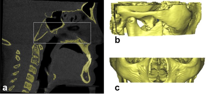
Selection of volume of interest (VOI), (a) cropping volume based on landmarks and boundary definitions (b) cropped VOI shown in lateral view (c) cropped VOI shown in coronal view.

The volume is cropped using Equation (A29), as shown in Figure A3.

Where C2sp(y) is extracted using Equation (A21), ANS(y) is extracted from Equation (A7), PNS(z) is extracted from Equation (A6) and N3³³ (z) extracted fromEquation (A16).

The left- and right-most lateral points on Zygomatic arch in VOI are the left Zygomatic and right Zygomatic landmarks, respectively. Hence, these can be detected by computing the left most point and right most point in the volume V1.

The landmark Condylion also exists in the same VOI V1. The left-most disconnected component of the inferior-most axial slice of VOI V1 is obtained as shown in Figure A4a. A mask is generated using the left, right and top boundaries of the disconnected component including inferior boundary till the end of the slice as shown in Figure A4b.

Figure A4.

Condylion landmark detection (a) left-most disconnected component of axial slice of the cropped VOI as referred from the (b) and shows Condylion region in axial view; (b) generated mask based on the boundaries of (a); (c) projected view of the logical addition on the axial slice; (d) logical addition of slices visualized in coronal view for the extraction of Condylion region; (e) Condylion region after removal of noise (f) 3D view of Condylion region with landmark plotted.

The generated mask was logically multiplied over the last slices with 3 mm range which is approximately 12 slices of 0.25 mm resolution in V1 and all these slices were projected on one axial slice as shown in Figure A4c.The inferior row of the Figure A4a was considered as the starting slice and the inferior row of Figure A4c was considered as the end slice of Condylion region in coronal view. The volume obtained in between the start and end slices of the coronal view are further used to detect Condylion landmark. Figure A4d was obtained by logical addition of the coronal slices from start slice to end slice. Figure A4e was obtained by extracting the left-most disconnected components of the Figure A4d using morphological operations. Condylion landmark is identified as the superior-most point in the Figure A4e. A similar process is applied to identify the right Condylion landmark.

The other two bilateral landmarks such as Gonion and R1 were obtained by extraction of the other VOI using Equation (A30) as shown in the Figure A5.

Figure A5.

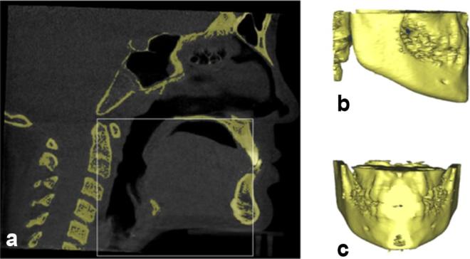
Selection of volume of interest (VOI) (a) cropping volume based on landmarks and boundary definitions (b) VOI in lateral view (c) VOI in coronal view 

$${\displaystyle \begin{array}{ll}\mathrm{V}2& =S\left(x,y,z\right),x\in \left[1,l\right],y\in \left[C2sp\left(y\right),ANS\left(y\right)\right],\\ & z\in \left[PNS\left(z\right),n\right]\end{array}}$$

Where C2sp(y) is extracted using Equation (A21), ANS(y) is extracted using Equation (A7) and PNS (z) is extracted using Equation (A6).

Gonion landmark is identified by using the VOI V2. The mask is generated using the initial axial slice of the VOI V2. The disconnected component visualized at extreme left of the initial axial slice was considered and a rectangular mask is generated using the boundaries of the same disconnected component as shown in Figure A6a. The mask is logically multiplied with all the slices in axial orientation of the VOI. Figure A6b–e shows a few axial slices arbitrarily numbered as 1, 50, 100 and 150 of same VOI V2. A graph is drawn by taking the z-axis co-ordinates of the inferior points of disconnected components in each slice of the VOI as shown in Figure A6f. The origin was considered at the location of intersection of maximum of the y-axis and minimum of x-axis irrespective of skull’s dimension. The Euclidean distances were calculated from the origin to the points in the graph. The point corresponding to the shortest distance is identified as Gonion landmark. The similar methodology is used to find the other side of the Gonion landmark.

Figure A6.

Detection of Gonion landmark (a) generated mask (b) initial axial slice of the VOI V2 after multiplication of mask (c) axial slice numbered 50 (d) axial slice numbered 100 (e) axial slice numbered 150 (f) graph obtained by using the inferior points of the slices (X-axis represents slice number, Y-axis represents inferior point in each slice); (b), (c), (d) and (e) are the exemplary slices in coronal view representing the detection of inferior-most point of the disconnected component (g) 3D view of Gonion region with plotted landmark

The landmark R1 also exists in the volume V2. A mask is generated using the initial slice of the volume V2. The disconnected component visualized at extreme right of the first slice is considered and a rectangular mask is generated using the boundaries of the same disconnected component as shown in Figure A7b. The generated mask is logically multiplied with all the axial slices of the VOI V2. The superior-most point of the disconnected component in the axial view of initial slice was extracted. The coronal slices from the detected superior-most point in axial slices were processed to detect the landmark R1. A slice was determined where a point exist showing the connecting of the inferior-most and superior-most disconnected components. This point is detected as landmark R1 the process is also shown through Figure A7c–f shows the detected landmark on the volume V2. The similar methodology is used to find the other side of the R1 landmark.

Figure A7.

Detection of landmark R1 (a) initial slice in axial view of volume of interest V2 (b) generated mask (c) coronal slice numbered 1 (d) coronal slice numbered 5 (e) coronal slice numbered 10 (f) R1 landmark on volume V2; (c), (d), (e) are the exemplary slices in coronal view representing the process of detection of R1 landmark. (c) Shows only superior-most point of disconnected point while (d) shows both the disconnected component where a connecting point of inferior-most and superior-most point of two different disconnected components can be detected. (e) Shows the joint between those disconnected components which is desirable for the R1 landmark.

FUNDING

The authors would also thank Dr Shilpa Kalra, and Dr Sushma Chaurasia at All India Institute of Medical Sciences—Centre for Dental Education and Research, New Delhi, India for manual plotting landmark on the data sets used in the study.

Ethical approval

The study was approved by institutional ethics committee (Ref. No. IEC/NP-185/2013 & RP-11/06.05.2013).

REFERENCES

- 1.Vasamsetti S, Sardana V, Kumar P, Kharbanda OP, Sardana HK. Automatic landmark identification in lateral cephalometric images using optimized template matching. J Med Imaging Health Inform 2015; 5: 458–70. doi: https://doi.org/10.1166/jmihi.2015.1426 [Google Scholar]
- 2.Shahidi S, Shahidi S, Oshagh M, Gozin F, Salehi P, Danaei SM. Accuracy of computerized automatic identification of cephalometric landmarks by a designed software. Dentomaxillofac Radiol 2013; 42: 20110187: 20110187. doi: https://doi.org/10.1259/dmfr.20110187 [DOI] [PMC free article] [PubMed] [Google Scholar]
- 3.Chien PC, Parks ET, Eraso F, Hartsfield JK, Roberts WE, Ofner S. Comparison of reliability in anatomical landmark identification using two-dimensional digital cephalometrics and three-dimensional cone beam computed tomography in vivo. Dentomaxillofac Radiol 2009; 38: 262–73. doi: https://doi.org/10.1259/dmfr/81889955 [DOI] [PubMed] [Google Scholar]
- 4.Baumrind S, Frantz RC. The reliability of head film measurements. Am J Orthod 1971; 60: 111–27. doi: https://doi.org/10.1016/0002-9416(71)90028-5 [DOI] [PubMed] [Google Scholar]
- 5.Cheng E, Chen J, Yang J, Deng H, Wu Y, Megalooikonomou V, et al. . Automatic dent-landmark detection in 3-D CBCT dental volumes. Conf Proc IEEE Eng Med Biol Soc 2011; 2011: 6204–7. doi: https://doi.org/10.1109/IEMBS.2011.6091532 [DOI] [PubMed] [Google Scholar]
- 6.Gupta A, Kharbanda OP, Sardana V, Balachandran R, Sardana HK. A knowledge-based algorithm for automatic detection of cephalometric landmarks on CBCT images. Int J Comput Assist Radiol Surg 2015; 10: 1737–52. doi: https://doi.org/10.1007/s11548-015-1173-6 [DOI] [PubMed] [Google Scholar]
- 7.Keustermans J, Mollemans W, Vandermeulen D, Suetens P. Automated cephalometric landmark identification using shape and local appearance models pattern recognition (ICPR), 2010 20th international conference on. 2010;: p.2464–7. [Google Scholar]
- 8.Keustermans J, Smeets D, Vandermeulen D, Suetens P. Automated cephalometric landmark localization using sparse shape and appearance models : Suzuki K, Wang F, Shen D, Yan P, Machine learning in medical imaging: Second International Workshop, MLMI 2011, held in conjunction with MICCAI 2011, Toronto, Canada, September 18, 2011. Proceedings. Berlin, Heidelberg: The British Institute of Radiology.; 2011. 249–56. [Google Scholar]
- 9.Shahidi S, Bahrampour E, Soltanimehr E, Zamani A, Oshagh M, Moattari M, et al. The accuracy of a designed software for automated localization of craniofacial landmarks on CBCT images. BMC Med Imaging 2014; 14: 32. doi: https://doi.org/10.1186/1471-2342-14-32 [DOI] [PMC free article] [PubMed] [Google Scholar]
- 10.Zheng P, Belaton B, Zaharudin R, Irani A, Rajion ZA. Computerized 3D craniofacial landmark identification and analysis. Electronic Journal of Computer Science and Information Technology 2011; 1. [Google Scholar]
- 11.Codari M, Caffini M, Tartaglia GM, Sforza C, Baselli G. Computer-aided cephalometric landmark annotation for CBCT data. Int J Comput Assist Radiol Surg 2017; 12: 113–21. doi: https://doi.org/10.1007/s11548-016-1453-9 [DOI] [PubMed] [Google Scholar]
- 12.Gupta A, Kharbanda OP, Sardana V, Balachandran R, Sardana HK. Accuracy of 3D cephalometric measurements based on an automatic knowledge-based landmark detection algorithm. Int J Comput Assist Radiol Surg 2016; 11: 1297–309. doi: https://doi.org/10.1007/s11548-015-1334-7 [DOI] [PubMed] [Google Scholar]
- 13.Makram MKH. Reeb graph for automatic 3D cephalometry. int J Image Process 2014; 8: 17–65. [Google Scholar]
- 14.Gupta A, Kharbanda OP, Balachandran R, Sardana V, Kalra S, Chaurasia S, et al. . Precision of manual landmark identification between as-received and oriented volume-rendered cone-beam computed tomography images. Am J Orthod Dentofacial Orthop 2017; 151: 118–31. doi: https://doi.org/10.1016/j.ajodo.2016.06.027 [DOI] [PubMed] [Google Scholar]
- 15.Guijarro-Martínez R, Swennen GR. Three-dimensional cone beam computed tomography definition of the anatomical subregions of the upper airway: a validation study. Int J Oral Maxillofac Surg 2013; 42: 1140–9. doi: https://doi.org/10.1016/j.ijom.2013.03.007 [DOI] [PubMed] [Google Scholar]