Whole-brain calcium imaging reveals an intrinsic functional network in Drosophila

Summary

A longstanding goal of neuroscience has been to understand how computations are implemented across large-scale brain networks. By correlating spontaneous activity during “resting-states”[1], studies of intrinsic brain networks in humans have demonstrated a correspondence with task-related activation patterns[2], relationships to behavior[3], and alterations in processes such as aging[4] and brain disorders[5], highlighting the importance of resting state measurements for understanding brain function. Here, we develop methods to measure intrinsic functional connectivity in Drosophila, a powerful model for the study of neural computation. Recent studies using calcium imaging have measured neural activity at high spatial and temporal resolution in zebrafish, Drosophila larvae, and worms[6–10]. For example, calcium imaging in the zebrafish brain recently revealed correlations between the midbrain and hindbrain, demonstrating the utility of measuring intrinsic functional connections in model organisms[8]. An important component of human connectivity research is the use of brain atlases to compare findings across individuals and studies[11]. An anatomical atlas of the central adult fly brain was recently described[12]; however, combining an atlas with whole-brain calcium imaging has yet to be performed in vivo in adult Drosophila. Here, we measure intrinsic functional connectivity in Drosophila by acquiring calcium signals from the central brain. We develop an alignment procedure to assign functional data to atlas regions and correlated activity between regions to generate brain networks. This work reveals a large-scale architecture for neural communication and provides a framework for using Drosophila to study functional brain networks.

eTOC blurb

Mann et. al. provide methods to quantify functional connectivity in Drosophila using wholebrain calcium imaging and tools for brain atlas registration. Their method confirms known relationships between brain regions and identifies previously unknown connections. These data lay the groundwork for future research on brain network organization.

Results

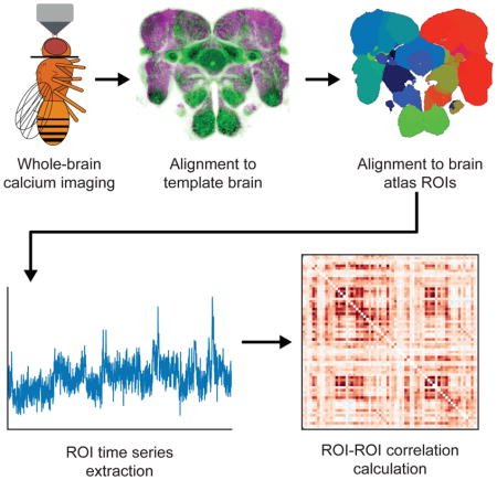
Overview of data collection and analysis pipeline

To build functional brain networks in Drosophila, we developed a streamlined method of imaging and template registration to reliably extract and compare calcium signals across animals. First, animals that expressed the calcium indicator GCaMP6m[13] and the red fluorescent protein tdTomato[14] pan-neuronally were head-fixed, immobilized, and dissected to expose the central brain. Animals were then imaged in the absence of sensory stimuli using a high-speed resonant scanning two-photon system to acquire whole-brain calcium signals (2.6×2.6×7.5μm voxels, 1.91 Hz) and a high-resolution anatomical scan (0.65×0.65×1μm voxels) using the tdTomato signal. We then developed a pipeline to align a standard atlas of annotated brain regions[12] to each animal’s anatomy using an established template brain[15]. Finally, after extracting calcium signals from each atlas region, we correlated the time series between each region pair for each fly, providing quantifications of functional connectivity that could be mapped to the current consensus on the position and nomenclature of the fly neuropil.

Brain atlas alignment

We first optimized a new alignment protocol to extract functional data from atlas regions of interest (ROIs)[12]. Previous work used the Computational Morphometry Toolkit (CMTK) to align fixed, stained brains[16, 17], but using CMTK to align a structural atlas to functional data was previously unexplored. Direct alignment of the template brain[15] to either live anatomical scans or post-hoc neuropil-stained brains proved unreliable. Therefore, we developed a three-step alignment protocol (Figure 1A). First, a live “mean brain” was generated by aligning anatomical scans of eight brains and averaging their intensity profiles. Second, the template[15] was aligned to the mean brain, producing warp parameters that were applied to the atlas ROIs[12], creating the mean-aligned atlas (Figure 1A). Third, the mean brain was aligned to each animal’s anatomical scan, producing warp parameters that were applied to the mean-aligned atlas, creating animal-specific atlases (Figure 1A). Thus, after performing this alignment protocol, atlas ROIs were warped to the morphology of each animal’s brain, allowing us to extract calcium signals from ROIs in each animal.

Figure 1. Alignment of brain atlas to functional brain data.

(A) Schematic of three-step brain alignment. (1) Eight anatomical scans of a myr:tdTomato channel from live animals were aligned to each other and averaged to generate the “mean” brain. (2a) Template brain was aligned to the mean brain. (2b) Fly brain atlas was warped to the mean brain according to the parameters in (2a). (3a) Mean brain was aligned to each individual live anatomical scan. (3b) Fly brain atlas was warped to each individual animal according to the parameters in (3a). (3c) Fly brain atlas was downsampled to the functional resolution scan and eroded by one voxel at the edges of each ROI. Examples shown in (A) are single slices used only for visualization purposes. (B) Example of the calculation of overlap shown in d, f, and h. From left to right: Post-alignment of template brain (green) to mean brain, showing ROIs from the fly brain atlas (Atlas-ROI, yellow) corresponding to the mushroom bodies (MB). Mean brain (magenta) with manually drawn ROIs corresponding to the MB of the same section (Mean-ROI, blue). Overlay of the fly brain atlas ROIs and manually drawn ROIs. Overlay of the fly brain atlas and manual ROIs also depicting the overlap (AtlasROI∩MeanROI) (red). (C) Example overlays of template (green) and mean brain (magenta) with Atlas-ROIs (yellow) from the MBs and the fan-shaped body (FB) anterior to posterior (left to right). (D) Quantification of overlap between atlas-ROIs and mean-ROIs expressed as a percent of in-plane area of the atlas-ROI. ROIs were drawn at 20μm intervals (MB, 26 in-plane ROIs, 13 in each hemisphere) and 15μm intervals (FB, 4 in-plane ROIs). (E) Example overlays of mean brain (magenta) and live anatomical scan (Anat-tdTomato, green) with Mean-ROIs (yellow) from the MBs and the FSB body anterior to posterior (left to right). (F) Quantification of overlap between mean-ROIs and live-ROIs expressed as a percent of in-plane area of the mean-ROI. (G) Example overlays of eroded fly brain atlas ROIs (Eroded-ROI, yellow) and functional data (Func-GCaMP). (H) Quantification of overlap between eroded-ROIs and func-ROIs. Note that no images used to create the “mean” brain were used to quantify registration quality. For panels D, F, and H, individual points represent the overlap for each in-plane ROI. Data is plotted as the mean ± SEM. Scale bars are 100μm. See also Figure S1.

Description of ROI terminology: Mean-ROI, manually drawn ROIs from the mean brain; Atlas-ROI, ROIs from the atlas; Live-ROI, manually drawn ROIs from live anatomical data; Func-ROI, manually drawn ROIs from functional GCaMP data (Func-ROI); Eroded_Atlas-ROI, ROIs from the atlas that have been resampled to functional resolution and eroded by one voxel.

To assess alignment quality, we compared aligned atlas ROIs to those manually drawn from the mushroom bodies (MB) and the fan-shaped body (FB) at various depths (Figure 1B), as these regions span significant portions of the brain and have easily identifiable edges. First, we quantified the overlap of each ROI drawn on the mean brain (Mean-ROI) to the corresponding atlas ROIs (Atlas-ROI) (Figure 1C, D; Figure S1). There was extensive overlap between the manually-drawn Mean-ROI and Atlas-ROI (mean ± SEM 88% ± 0.1). Second, we quantified the overlap of each ROI drawn on the mean brain (Mean-ROI) to the corresponding ROI drawn on two live anatomical scans (Live-ROI). These also showed high overlap (mean ± SEM 95.2% ± 0.5; N = 2 brains; Figure 1E, F; Figure S1). Finally, we compared the overlap of the atlas ROIs (Atlas-ROI) to those drawn on functional data (Func-ROI). As functional data was acquired at a lower spatial resolution than the structural data, slightly diminishing registration quality (Figure S1), we eroded the edges of each atlas ROI by one voxel after resampling them to functional resolution. This resulted in high overlap between the eroded atlas ROIs and functional ROIs (mean ± SEM 95.9% ± 0.8; Figure 1G, H; N = 2 brains). Thus, this alignment protocol allowed functional data to be reliably extracted from atlas regions.

Analysis of ROI-specific calcium signals

We next correlated the extracted time series between pairs of ROIs (Figure 2A). As expected, large calcium excursions that spanned multiple ROIs produced strong correlations (Figure 2B). We also observed strong correlations between ROIs that lacked such excursions (Figure 2C). Lastly, we observed that some ROIs were not significantly correlated (Figure 2D). This demonstrates that correlations between ROIs can arise from multiple features in calcium signals and are selective to particular pairs of ROIs. Examining individual voxel contributions to ROI calcium signals, we found that voxel signals within each ROI were well represented by the average ROI signal and were reasonably homogenous (Figure 2SA; Figure S2B), although future work generating functional connectivity-based atlases could potentially increase signal homogeneity within ROIs.

Figure 2. Functional imaging data and time series correlations between regions.

(A) Example ΔF/F traces of atlas ROIs (N = 61) from a single fly for 8.5 minutes (half of an imaging session). Numbers to the right of each trace correspond to those used for correlations in B–D. (B–D) Scatter plots of ΔF/F values from left, with top trace (ordinate) plotted against the bottom trace (abscissa) and their corresponding Pearson’s correlation values calculated from correlating the time series between ROIs (R). (B) Example of highly-correlated brain regions that show large calcium excursions (arrows show example excursion from both regions). (C) Example of highly-correlated brain regions that do not show large calcium excursions. (D) Example of weakly-correlated brain regions. Regions shown are (1) right mushroom body medial lobe (MBML_R), (2) right antennal lobe (AL_R), (3) right superior medial protocerebrum (SMP_R), (4) fan-shaped body (FB), (5) right inferior posterior slope (IPS_R), (6) ellipsoid body (EB). See also Figure S2.

Quantification of whole-brain functional connectivity

We next extended these time series correlations to include all atlas ROI pairs, forming a correlation matrix that represents the functional connectivity of each ROI-pair for individual flies (Figure S2C). We performed this analysis on 18 flies, each imaged for 17 minutes (2000 time points). The resulting maps were highly stereotyped (Figure S2D). There were strong correlations between correlation matrices obtained from any two flies (mean ± SEM R = 0.64 ± 0.01; Figure S2E) and from individual flies imaged at different times (average ± SEM R = 0.88 ± 0.03; Figure S2E). Examining individual functional connections, we found that approximately 27% (N = 501) of possible connections between ROIs were significantly correlated (Figure 3A; Figure S2F–H). Simulated data confirmed that functional connectivity was not an artifact of our imaging methods, as simulations produced only one significant correlation (Figure S3A–C). We also examined the frequencies over which these correlations emerged (Figure S3D, E) and found that the correlation values were highest at frequencies approximately one order of magnitude lower than our imaging rate (i.e., 0.01 – 0.1 Hz), which are well-sampled by our imaging methods. To examine the extent of each region’s functional connectivity to the rest of the brain, we measured the mean correlation of each ROI to every other ROI (Figure 3B). These mean correlations spanned approximately an order of magnitude; some regions, such as the superior medial protocerebrum (SMP), exhibited high functional connectivity to the rest of the brain; others, such as the gorget (GOR), did not exhibit significant functional connectivity with any part of the brain. Finally, we examined how differences in ROI size influenced functional connectivity. There was a correlation between the number of voxels in each ROI and its average connectivity to the rest of the brain (r = 0.46, p < 0.001), possibly reflecting noisier signals due to diminished averaging across voxels in smaller ROIs. However, there was no relationship between the number of voxels in each ROI and the number of significant connections an ROI had in total (r = 0.05, p = 0.71). This suggests that larger ROIs may have higher average functional connectivity, but not necessarily a larger number of connections.

Figure 3. Whole-brain intrinsic functional connectivity.

(A) Significant functional connections between brain atlas regions (N = 61 ROIs). For significant functional connections, the strength of each connection represents the Fisher transformed correlation value (z) between atlas regions, averaged across all N = 18 animals. Non-significant functional connections are presented as white cells. Significance of functional connections was calculated using a one-sample t-test against zero across all flies at α = 0.001 Bonferroni-corrected for all connections tested (number of connections = 1830, p < 5.46e–7). (B) Average Fisher-transformed correlation values of each atlas region to all other regions. Bars are plotted as mean ± SEM. Significance of ROI functional connectivity was calculated using a one-sample t-test against zero across all flies at α = 0.001 Bonferroni-corrected for all regions tested (number of regions = 61, p < 1.64e–5). *p < 0.001. See also Figures S2–S3, Table S1.

Deriving functional networks in Drosophila to reveal the intrinsic organization of the brain

We next used these correlation matrices to derive a network, where ROIs represent network nodes and the connections between them represent network edges. We visualized the strongest 3%–20% of significant functional connections (Figure 4A; Figure S4). Strikingly, we observed some functional connections that were predicted from previous work, as well as a number of new functional connections that were not anticipated. For example, regions involved in olfactory processing (antennal lobe (AL), lateral horn (LH), MB, SMP, superior lateral protocerebrum (SLP), crepine (CRE)) showed a high degree of interconnectivity, suggesting that intrinsic functional connectivity may capture known processing streams. We also observed functional connections between previously unassociated regions, such as the SMP and FB and a bilateral functional connection between the left and right anterior ventro-lateral protocerebrum (AVLP).

Figure 4. Organizational properties of intrinsic brain networks network in Drosophila.

(A) Fly brain network with labeled atlas regions represented as circles and functional connections between them represented as lines. Atlas regions are shown over a schematized fly brain with optic lobes (lighter, lateral) antennal lobes and mushroom bodies (darker, dorsal), and esophageal foramen (white, medial). Here, the top 3% of significant functional connections in the central fly brain are shown. The 3% cutoff corresponds to a 0.61–1.03 range of correlation values. It should be noted that this cutoff was chosen only for visualization purposes. Groups of brain regions are colored as follows: left olfactory-related regions (blue), right olfactory-related (green), midline regions (magenta), all other regions (purple). Functional connections between brain regions of the same group are colored the same as the regions themselves, while functional connections between regions of different groups are colored grey. Functional connections are weighted according to their average functional connectivity strength (reflected in the width of the line). See also Figure S4. (B) Lateralization of functional connectivity within and between hemispheres. (Left) Connectivity is presented as the average Fisher z-transformed values (i.e., connectivity calculated for each fly and averaged across flies) between groups of regions depending on hemispheric location (mean ± SEM across flies). For each fly, intra-hemispheric functional connectivity (Intra-Left, Intra-Right) was calculated by averaging functional connectivity values within left and right hemisphere atlas regions, respectively. Inter-hemispheric functional connectivity (Inter-Hemispheric) was calculated by averaging functional connectivity values between left and right hemisphere atlas regions. Homologous region functional connectivity (Homologous) was calculated by identifying regions with left-right pairs and averaging functional connectivity over these pairs. Midline functional connectivity (Midline) was calculated by averaging functional connectivity between midline regions and lateral brain regions. (Right) Individual animal values (N = 18) for data presented in (B, Left). (C) Midline functional connections, with similar coloring as in (A). Here, all significant midline functional connections are presented at a fixed connection width (i.e., functional connectivity strength is not incorporated into line width).

The fly brain is bilaterally symmetric, yet how this anatomical symmetry might be reflected in functional relationships between hemispheres and midline structures is unknown. To examine the lateralization of intrinsic functional connections, we compared correlation values between pairs of ROIs based on their hemispheric location and found that the strength of functional connectivity differed across hemispheric locations (Figure 4B; F(4,68) = 30.69, p < 0.001). In particular, while functional connectivity within left and right hemispheres was similar (t(17) = 0.54, p = 0.60), intra-hemispheric functional connectivity was greater than inter-hemispheric functional connectivity (intra-left compared to inter-hemispheric: t(17) = 5.49, p < 0.001; intra-right compared to inter-hemispheric: t(17) = 3.66, p = 0.002). Additionally, examining sub-types of inter-hemispheric functional connections, we found that functional connectivity was highest for homologous region pairs compared with other types of functional connections (all p’s < 0.001), raising the possibility that communication occurs between homologous ROIs across hemispheres. We also examined the relationship between these lateralized connectivity patterns and ROIs at the midline of the brain, which have been considered points of convergence in neural processing streams[18, 19]. In aggregate, functional connectivity between midline structures and lateral brain regions was similar to that of all inter-hemispheric functional connections (t(17) = −0.80, p = 0.43). Remarkably, however, when examining the number of significant functional connections between individual midline and lateral ROIs (N = 71 connections), we found dramatic differences in the distribution of functional connections across midline regions (χ² = 68.70, p < 0.001; Figure 4C). In particular, the FB and ellipsoid body (EB) had many distributed functional connections (N = 31 and 18, respectively), while the saddle (SAD), prow (PRW), noduli (NO) and protocerebral bridge (PB) (N = 5, 7, 3, and 7, respectively) had very few lateral functional connections and the gnathal ganglion (GNG) had none. Moreover, the lateral regions that were functionally connected to the midline overlapped significantly. Specifically, 94% of the functional connections (N = 33) made by the EB, NO, PB, SAD and PRW were also functionally connected to the FB. Thus, the FB and EB exhibited a majority of functional connections made to each hemisphere and these functional connections sampled a specific subset of lateral brain regions, suggesting that these two midline regions play an important role in inter-hemispheric communication.

Discussion

These data demonstrate the development of novel analysis tools to quantify intrinsic functional connectivity in the central brain of Drosophila. We developed protocols to acquire and register functional calcium data to a standard brain atlas. This method of acquisition, registration, and processing is widely applicable to whole-brain calcium imaging and is thus compatible with a range of experiments, including identifying functional maps for many types of stimuli and behaviors. Using these methods, we quantified properties of intrinsic functional networks in the fly brain. This revealed large-scale network organization, such as lateralization of functional connectivity, and discovered potential new roles for brain regions based on their functional connections.

Methods for quantifying intrinsic brain network functional connectivity

Here, we introduce a pipeline to reliably quantify functional connections between brain regions in Drosophila. Our approach offers three critical advantages. First, it provides a means to align functional data to a common brain template and atlas, allowing datasets to be directly compared. Second, it employs commonly used tools for image registration and analysis that can be widely applied. Third, our analyses demonstrate that intrinsic functional correlations emerge at low frequencies, a phenomenon also observed in fMRI-based connectivity. As a result, it is possible to acquire such functional measurements at high spatial resolution using commercially available laser scanning two-photon microscopes. Our results also suggest that imaging methods with higher spatial resolution may be more useful for this approach than those with greater temporal resolution. Therefore, slower GCaMP variants may be more appropriate for measuring intrinsic connectivity, although this might not be the case for stimulus-dependent connectivity where higher frequency oscillations could dominate. In this case, faster imaging could be combined with a head-fixed setup that allows for freedom of motion to examine how stimuli and behavior alter functional connectivity. Moreover, a finer parcellation of the brain atlas may allow for the identification of functional connections that would otherwise be undetected, such as activity in sub-regions of the ellipsoid body during navigation[20]. Finally, while our current methodology cannot provide information about the directionality of functional connections, future work using high speed imaging combined with indicators with faster kinetics could allow quantification of directed brain networks.

Intrinsic functional connectivity reveals functional relationships in the brain

Quantifying intrinsic functional connections between brain regions allows assessments of brain network properties based on correlations of their spontaneous, ongoing activity, rather than their anatomy or synaptic connectivity. Anatomical reconstruction of the fly brain has been used to measure structural connectivity based on neuronal morphology[18]. While much of our functional data map onto known structural connections, we observe both strong and weak functional connections not predicted by anatomy. For example, the dorsal/superior protocerebrum (SMP) and the fan shaped body (FB) are strongly interconnected based on both functional and structural measurements, while the noduli (NO) are weakly functionally connected to other brain regions by both measures (Figure 3B)[16]. Conversely, structural connectivity predicts a moderate level of functional interconnectedness in the mushroom bodies[18], while our functional analysis shows that the medial lobe of the mushroom bodies (MB_ML) is highly correlated with much of the fly brain. Thus, while structural data can predict some functional connections, functional connectivity can arise independent of direct anatomical constraints, perhaps reflecting indirect connections.

We speculate that regions implicated in similar functional and processing roles are strongly functionally connected in a task free state. For example, regions involved in olfactory processing are highly interconnected and represent some of the strongest observed correlations, even in the absence of olfactory input (Figures 3A, 4A). We also discovered previously unknown functional relationships between regions. The FB, which is involved in visual learning and shape recognition[21, 22], is highly correlated with olfactory processing centers, such as the MB. The FB also responds to a wide range of visual stimuli during flight, suggesting that it plays a role in flight motor control[23]. As olfactory cues can also direct flight, in addition to visual feedback[24, 25], the observed strong functional connections with the MB may reflect the FB’s role in integrating multimodal signals to control flight. Conversely, the AVLP, which has been shown to be involved in auditory processing[26], shows very low correlations with other auditory regions, such as the AMMC, and instead is highly correlated with its homolog, suggesting additional roles for these regions.

Defining the global architecture of lateralization

Our whole-brain imaging approach allowed us to examine large-scale network properties, such as lateralization. We find stronger functional connectivity within hemispheres compared to functional connections between hemispheres (Figure 4B). Interestingly, we also find that functional connectivity between homologous pairs is higher than that observed for intra-hemispheric functional connectivity. This suggests that specific cross-hemisphere communication between analogous brain regions is high, in accordance with work in humans[27], perhaps reflecting parallel processing streams in the hemispheres from common inputs or cross-talk between homologous regions. In addition, while we find that midline regions have similar functional connectivity strength to inter-hemispheric connectivity, we also observe that a subset of midline regions plays a prominent role in the network. Specifically, we find that the FB and EB have widespread functional connections across the brain, while the remaining midline brain regions have few functional connections. Thus, the FB and EB may be particularly well-suited to integrate information across hemispheres, while other midline regions may have more specialized roles. Future work should consider how this functional description of hemispheric architecture maps onto descending neuron populations to guide behavior.

Applications of functional network analysis in Drosophila

While much of our understanding of functional brain networks has come from research in humans, our ability to perform invasive experiments to manipulate networks in humans is limited. We suggest that Drosophila is a powerful model for the study of brain networks. First, individual neurons, clusters of neurons, or whole brain regions can be manipulated, through a combination of genetic and optical methods, on both short and long time scales, allowing us to probe dynamic network changes as individual elements are perturbed. Such experiments could, for example, guide understanding of brain lesions by causally probing the relationship between a lesioned region’s connectivity and changes in network organization[28]. Second, mutations that affect behavior or model brain disorders in flies could be combined with this approach to use network architecture as a phenotypic readout that extends our mechanistic understanding. In the future, we anticipate that exploring how cellular, genetic, and physiological manipulations alter intrinsic brain network architecture in the fly will make important advances in our understanding of brain organization and behavior.

STAR Methods

CONTACT FOR REAGENT AND RESOURCE SHARING

Further information and requests for resources and reagents should be directed to and will be fulfilled by the Lead Contact, Thomas R. Clandinin (trc@stanford.edu).

EXPERIMENTAL MODEL AND SUBJECT DETAILS

Fly stocks

Strains are provided in the Key Resources Table. All animals used in experiments were females of the genotype w+; UAS-myr::tdTomato/UAS-GCaMP6m; nSyb-Gal4/+. Flies were raised on molasses medium at 25°C with a 12/12-hour light/dark cycle. Flies were housed in mixed male/female vials and 5-day old females were selected for imaging.

KEY RESOURCES TABLE.

REAGENT or RESOURCE	SOURCE	IDENTIFIER
Deposited Data
Raw and analyzed data	This paper	http://dx.doi.org/10.17632/8b6nw2xxhn.1
Experimental Models: Organisms/Strains
D. melanogaster w*; P{10XUAS-IVS-myr::tdTomato}attP40	Bloomington Drosophila Stock Center	FBst0032222, RRID:BDSC_32222
D. melanogaster w1118; P{20XUAS-IVS-GCaMP6m}attP40	Bloomington Drosophila Stock Center	FBst0042748, RRID:BDSC_42748
D. melanogaster w1118; P{GMR57C10-GAL4}attP2	Bloomington Drosophila Stock Center	FBst0039171, RRID:BDSC_39171
Software and Algorithms
CMTK	NITRC	https://www.nitrc.org/projects/cmtk/, RRID:SCR_002234
AFNI	[29]	https://afni.nimh.nih.gov/, RRID:SCR_005927
FSL	[30]	https://fsl.fmrib.ox.ac.uk/fsl/, RRID:SCR_002823
Python 2.7	Python Software Foundation	http://www.python.org, RRID:SCR_008394
Custom-built Python code	This paper	https://github.com/cgallen/MannGallen_2017_CurrentBiology
Prism 6.0h	GraphPad	https://www.graphpad.com/scientific-software/prism/, RRID:SCR_002798
Other
Template brain and atlas	Virtual Fly Brain	http://www.virtualflybrain.org/

METHOD DETAILS

Calcium imaging

Preparation

All animals were imaged on the fifth day post-eclosion. Flies were cold-anaesthetized by putting them in an empty vial and chilling them on ice for approximately one minute. Flies were then inserted into a collar that fits around the cervix and provides a separate chamber for the head and the rest of the fly as previously described (Figure S1N–Q)[10]. Animals were immobilized using nail polish applied to the back of the head, to the proximal portions of the legs, and to the wings to prevent motion. Nail polish was applied via mouth pipette through a pulled glass capillary, allowing for precise application. Animals were gently dissected in cold fly saline (103 mM NaCl, 3 mM KCl, 5 mM TES, 1 mM NaH2PO4, 4 mM MgCl2, 1.5 mM CaCl2, 10 mM trehalose, 10 mM glucose, 7 mM sucrose, and 26 mM NaHCO3) lacking calcium or sugar. To expose the central brain, the proboscis, antennae, and surrounding cuticle were removed, as were the trachea and fat occluding the brain. The eyes and other cuticle were left intact. Flies were then transferred to a custom mount and perfused with complete saline bubbled with 95% O₂ and 5% CO₂.

Microscopy

Flies were imaged at room temperature on a Bruker Ultima system with resonant scanning capability, a piezo objective mount, and GaAsP type PMTs using a Leica 20× HCX APO 1.0 NA water immersion objective lens. GCaMP6m signals were excited with a Chameleon Vision II femtosecond laser (Coherent) at 920nm, and collected through a 525/50nm filter. Myr::tdTomato signals were excited at 920nm and collected through a 595/50nm filter. GCaMP6m was selected over other variants as its kinetics best matched our imaging rate. Both channels were collected in resonant scanning mode (8kHz line scan rate, bidirectional scanning). GCaMP6m functional data was volumetrically imaged at a resolution of 128×128 (2.6×2.6μm) with 25 z-sections (7.5μm steps with 2× frame averaging, effective frame rate ~50Hz). For high speed z-sectioning, a piezo mount was used to control the position of objective. Z-stacks were collected unidirectionally. While the entire fly CNS, including the cell body cortex and central neuropils, were imaged in these experiments, only voxels corresponding to the neuropil atlas were used in analyses. Neuropils are highly structured in Drosophila and represent the functional units of the fly CNS. As the central brain of the fly is estimated to have 100,000 neurons that span tens to hundreds of microns in length, with submicron scale processes, each neuron contributed signals to multiple voxels, and each voxel contained the signals from tens of neurons.

Each fly was imaged for two 17.4-minute sessions (2000 time points) in the absence of any sensory stimuli. Specifically, the imaging room was temperature controlled (70°F) and flies were imaged in complete darkness. Removal of antennae prevented possible olfactory or auditory inputs. Removal of the proboscis and immobilization of the legs prevented possible gustatory inputs and contact with tastants. Anatomical myr::tdTomato stacks were collected in resonant scanning mode immediately prior to each functional GCaMP6m imaging session. These anatomical scans were collected at a resolution of 512×512 (0.65×0.65μm) with 181 z-sections (1 μm steps with 32× frame averaging).

Data preprocessing

Alignment

All alignment was done on the anatomical scan using CMTK, via the munger wrapper with the parameters specified[17]. Specifically, alignment was performed using the munger parameters (-X 26 –C 8 –G 80 –R 4 –A ‘–accuracy 0.4’ –W ‘–accuracy 0.4’). The atlas was then warped with each specific set of warping parameters using the reformatx command (CMTK) with the –nn (nearest neighbor) flag to prevent errors in the edge assignment of the atlas. Both the template and the atlas used can be downloaded from the virtual fly brain project website (www.virtualflybrain.org).

For the generation of the mean brain, eight myr::tdTomato anatomical scans (collected as stated above), not included in our experimental dataset, were aligned to each other (seven brains to one seed brain) using the same CMTK parameters. The seed brain was determined by selecting the best aligned single anatomical scan from multiple flies and was collected with a voxel resolution of 0.62×0.62×0.6 μm. The process of averaging brains aligned to the seed brain to generate the mean brain produced better alignment to the template than the seed brain alone (data not shown). An average of each voxel was taken by loading these as a 4D hyper-stack in ImageJ and taking the mean value across the eight brains.

Motion correction

Functional data was motion corrected using the 3dvolreg command in AFNI[29]. First, a mean functional dataset for each fly was created by averaging the first 100 volumes, using AFNI’s 3dTstat command. To perform motion correction, each functional volume was then aligned to the mean functional using 3dvolreg. Each dataset was inspected visually for quality of motion correction and confirmation that the motion-corrected functional data was aligned to the live structural data.

Data exclusion

Data was excluded from both imaging runs (i.e., data not included in analyses presented here, N = 6) or one imaging run (N = 8) prior to calculation of correlation matrices for several reasons. These included data that could not be adequately aligned to the template brain, functional data that drifted beyond our initial imaging bounds in any dimension during the imaging session, excessive motion in functional data, and animals in which the esophagus or other structure occluded any part of the brain.

Additionally, fourteen atlas ROIs were not included in our functional connectivity analyses because we either did not image them in total (i.e., optic lobe ROIs, medulla, lobula, lobula plate, and accessory medulla) or the erosion process eliminated them from any single fly in our dataset, usually a result of their small size (i.e., bulb, cantle, left inferior posterior slope, left gall).

Functional connectivity and network analyses

ROI erosion

ROIs were eroded by one voxel (using the 3dmask_tool command in AFNI) after resampling them to functional resolution (using the 3dresample command in AFNI) to prevent incorrect assignment of edge voxels to ROIs. Erosion by one voxel was chosen to approximate our alignment error (Figure 1) and was limited by the fact that further erosion eliminated many ROIs.

Quantification of functional connectivity

Using the 3dmaskave command in AFNI, we then extracted calcium imaging signals from all voxels in an ROI and then averaged the time series across these voxels to produce a single time series for each ROI in each fly. We next computed correlations of the time series between each ROI pair using Pearson’s correlations and applying a Fisher z-transform to generate 61 × 61 correlation matrices for each fly that represent functional connectivity between ROIs.

ROI homogeneity was calculated with two methods. First, for each ROI and fly, we calculated the Pearson’s correlation between the time series of each voxel in that ROI and the average time series of that ROI (‘Voxel-Mean’; Figure S2A). Second, for each ROI and fly, we calculated the Pearson’s correlations between each voxel pair in that ROI (‘Voxel-Voxel’; Figure S2B). For each method, we then Fisher z-transformed the resulting correlation values and averaged across the voxels within each ROI to provide a summary statistic for each ROI and fly. One ROI in one fly was excluded from further analysis because it contained only one voxel.

Reliability of correlation matrices between and within flies was examined by quantifying the correlation of functional connectivity values across datasets. First, to examine reliability between animals, correlations of functional connectivity values were computed between all possible pairs of flies (N = 18 flies, N = 153 inter-animal correlations) and were averaged over all pairs. Second, to examine reliability within flies, we collected two imaging runs (N = 2000 timepoints each) on a subset of flies (N = 10). Correlations of functional connectivity values were computed between the two imaging runs for each fly and then averaged.

Examination of intrinsic network properties

We next examined various properties of functional connectivity to characterize large-scale intrinsic network organization in the fly brain. First, to examine the significance of individual functional connections across all animals, we conducted one-sample t-tests against a comparison value of zero on the Fisher-transformed correlation values for each connection pair across flies, to identify functional connections with significant positive or negative correlation values. We used stringent significance threshold of α = 0.001, Bonferroni-corrected for all functional connection pairs (N = 1830 possible connections for 61 brain regions; p < 5.46e–7). Second, we examined how functional connectivity strength differs depending on the hemispheric-location of functional connections. For each fly, we quantified right and left intra-hemispheric functional connectivity by averaging correlation values (i.e., Fisher z-transformed values) within all right (N = 28 ROIs) and left-hemisphere (N = 26 ROIs) regions, respectively.

We quantified inter-hemispheric functional connectivity by averaging correlation values between all right- and left-hemisphere region pairs. We quantified homologous pair functional connectivity by averaging correlation values between the same brain regions in the opposite hemispheres (N = 26 ROI pairs). We quantified midline functional connectivity by averaging correlation values between midline regions (N = 7 ROIs) and all other brain regions. To examine whether functional connectivity strength differed across these five categories, we conducted a repeated-measures ANOVA with a within-subjects factor of lateralization category. Post-hoc comparisons between category pairs were conducted with paired-samples t-tests.

Third, we examined regional differences in the number of functional connections between midline and lateral regions (e.g., number of significant functional connections passing a corrected p < 0.001). For each of the seven midline regions, we calculated the number of its functional connections to lateral (non-midline) regions. To examine whether these 71 functional connections were uniformly distributed across the seven midline regions, we conducted a chi-squared test on the number of lateral functional connections for each midline region.

Generation of simulated data and spectral analyses

To confirm that the observed significant functional connections were not spuriously caused by our imaging methods or sampling rate, we generated simulated time series based on properties of our real data from N = 18 flies. Specifically, for each fly, we generated ROI-specific time series of random data with the same mean and standard deviation as the real ROI time series. To simulate data with similar temporal properties as our calcium imaging signal, we convolved these simulated time series with the kinetic profile of GCaMP6m[13] (Figure S3B) using a sum of exponentials:

$$f(x)=e^{-0.696x}-e^{-4.5x}$$

In particular, the initial random data were scaled such that the simulated data had the same mean and standard deviation as the real ROI time series after convolution. We repeated this procedure 1000 times for each fly, thus generating a dataset of 18000 simulated time series for each ROI. For each simulated dataset, we computed the Pearson’s correlations between each ROI pair and applied a Fisher z-transform. Using an identical significance threshold as the real data, we then quantified the number of significant functional connections in each simulated dataset.

To examine the spectral properties of our data in relationship to our imaging methods, we applied a series of temporal filters (fifth-order Butterworth) spanning 0.1–0.9 Hz in 0.1 Hz steps to the ROI time series for each fly. After computing correlations between each ROI pair and applying a Fisher z-transform, we quantified the average functional connectivity across all ROI pairs. We then compared the average functional connectivity value for each filter to that from the unfiltered data (Figure S3D). We also computed the coherence, the spectral analog of cross-correlation, between each ROI pair for each fly (Figure S3E).

QUANTIFICATION AND STATISTICAL ANALYSIS

Quantification of ROI Homogeneity

Significance of ROI homogeneity was tested with one-sample t-tests of the average Fisher-transformed correlation values against a comparison value of 0 for N = 18 files. As this analysis was exploratory in nature, we report significant ROI functional connectivity that passes a p < 8.20e-4 threshold (α = 0.05, Bonferroni-corrected for 61 ROIs tested). Results are presented in Figures 2A and 2B and include mean ± SEM across flies.

Identification of functional connections

Significance of individual functional connection pairs was tested with one-sample t-tests of the Fisher-transformed correlation values against a comparison value of 0 for N = 18 flies. We report significant functional connections that pass a p < 5.46e-7 threshold (α = 0.001, Bonferroni corrected for 1830 comparisons for all possible ROI pairs). Results are presented in Figure 3A and include mean Fisher-transformed correlation values across flies. A similar approach was taken to identifying significant functional connections during data simulations. Example simulated data are presented in Figures S3A and S3C and include ROI time series and mean Fisher-transformed correlation values across flies, respectively. Significance of ROI functional connectivity (i.e., average functional connectivity of each ROI to the remaining 60 ROIs) was tested with one-sample t-tests of the average Fisher-transformer correlation values against a comparison value of 0 for N = 18 files. We report significant ROI functional connectivity that passes a p < 1.64e-5 threshold (α = 0.001, Bonferroni-corrected for 61 ROIs tested). Results are presented in Figure 3B and include mean ± SEM across flies.

Relationship between ROI size and connectivity

Correlations between ROI size and connectivity were calculated with Pearson’s correlations between the number of voxels in each ROI (averaged over flies) and (1) ROI functional connectivity (i.e., functional connectivity of each ROI to the remaining 60 ROIs, averaged over flies) and (2) the number of significant functional connections of each ROI. Results are presented in the Results section.

Examination of connectivity lateralization

Differences in functional connectivity depending on hemispheric location were tested with a repeated-measures ANOVA with a within-subjects factor of connectivity type (intra-hemispheric left, intra-hemispheric right, inter-hemispheric, homologous pairs, midline) for N = 18 flies. Post-hoc comparisons were conducted with paired-samples t-tests. Results are presented in Figure 4B and include mean ± SEM across flies (left) and individual flies (right). The ANOVA was performed in Prism.

Differences in the distribution of significant midline functional connections were conducted with a chi-squared test of the number of functional connections (N = 71) across the seven midline regions. All statistical tests were two-tailed. Significant midline connections are presented in Figure 4C.

DATA AND SOFTWARE AVAILABILITY

Data illustrating the alignment pipeline as well as sample functional imaging data and atlas ROIs can be found on Mendeley Data (http://dx.doi.org/10.17632/8b6nw2xxhn.1). Code using Python, AFNI[29], and FSL[30] to process functional data and generate ROI time series can be found at: https://github.com/cgallen/MannGallen_2017_CurrentBiology.

Supplementary Material

2. Table S1. Atlas region names, abbreviations, and groupings. Related to Figure 3.

Table of atlas regions. Left, regions sorted according to their atlas index. Right, regions sorted alphabetically by name.

Highlights.

• Tools for alignment of a brain atlas to live Drosophila

• Calcium imaging of the entire central brain of Drosophila

• Quantification of functional connectivity between brain regions in Drosophila

References

- 1.Power JD, Schlaggar BL, Petersen SE. Studying brain organization via spontaneous fMRI signal. Neuron. 2014;84:681–696. doi: 10.1016/j.neuron.2014.09.007. [DOI] [PMC free article] [PubMed] [Google Scholar]
- 2.Smith SM, Fox PT, Miller KL, Glahn DC, Fox PM, Mackay CE, Filippini N, Watkins KE, Toro R, Laird AR, et al. Correspondence of the brain’s functional architecture during activation and rest. Proc Natl Acad Sci USA. 2009;106:13040–13045. doi: 10.1073/pnas.0905267106. [DOI] [PMC free article] [PubMed] [Google Scholar]
- 3.Vaidya CJ, Gordon EM. Phenotypic variability in resting-state functional connectivity: current status. Brain Connect. 2013;3:99–120. doi: 10.1089/brain.2012.0110. [DOI] [PMC free article] [PubMed] [Google Scholar]
- 4.Chan MY, Park DC, Savalia NK, Petersen SE, Wig GS. Decreased segregation of brain systems across the healthy adult lifespan. Proc Natl Acad Sci USA. 2014;111:E4997–5006. doi: 10.1073/pnas.1415122111. [DOI] [PMC free article] [PubMed] [Google Scholar]
- 5.Fornito A, Zalesky A, Breakspear M. The connectomics of brain disorders. Nat Rev Neurosci. 2015;16:159–172. doi: 10.1038/nrn3901. [DOI] [PubMed] [Google Scholar]
- 6.Prevedel R, Yoon YG, Hoffmann M, Pak N, Wetzstein G, Kato S, Schrödel T, Raskar R, Zimmer M, Boyden ES, et al. Simultaneous whole-animal 3D imaging of neuronal activity using light-field microscopy. Nat Methods. 2014;11:727–730. doi: 10.1038/nmeth.2964. [DOI] [PMC free article] [PubMed] [Google Scholar]
- 7.Lemon WC, Pulver SR, Höckendorf B, McDole K, Branson K, Freeman J, Keller PJ. Whole-central nervous system functional imaging in larval Drosophila. Nature Communications. 2015;6:7924. doi: 10.1038/ncomms8924. [DOI] [PMC free article] [PubMed] [Google Scholar]
- 8.Ahrens MB, Orger MB, Robson DN, Li JM, Keller PJ. Whole-brain functional imaging at cellular resolution using light-sheet microscopy. Nat Methods. 2013;10:413–420. doi: 10.1038/nmeth.2434. [DOI] [PubMed] [Google Scholar]
- 9.Chhetri RK, Amat F, Wan Y, Höckendorf B, Lemon WC, Keller PJ. Whole-animal functional and developmental imaging with isotropic spatial resolution. Nat Methods. 2015;12:1171–1178. doi: 10.1038/nmeth.3632. [DOI] [PubMed] [Google Scholar]
- 10.Harris DT, Kallman BR, Mullaney BC, Scott K. Representations of Taste Modality in the Drosophila Brain. Neuron. 2015;86:1449–1460. doi: 10.1016/j.neuron.2015.05.026. [DOI] [PMC free article] [PubMed] [Google Scholar]
- 11.Stanley ML, Moussa MN, Paolini B. Defining nodes in complex brain networks. Frontiers in Computational Neuroscience. 2013:7. doi: 10.3389/fncom.2013.00169. [DOI] [PMC free article] [PubMed] [Google Scholar]
- 12.Ito K, Shinomiya K, Ito M, Armstrong JD, Boyan G, Hartenstein V, Harzsch S, Heisenberg M, Homberg U, Jenett A, et al. A systematic nomenclature for the insect brain. Neuron. 2014;81:755–765. doi: 10.1016/j.neuron.2013.12.017. [DOI] [PubMed] [Google Scholar]
- 13.Chen TW, Wardill TJ, Sun Y, Pulver SR, Renninger SL, Baohan A, Schreiter ER, Kerr RA, Orger MB, Jayaraman V, et al. Ultrasensitive fluorescent proteins for imaging neuronal activity. Nature. 2013;499:295–300. doi: 10.1038/nature12354. [DOI] [PMC free article] [PubMed] [Google Scholar]
- 14.Shaner NC, Campbell RE, Steinbach PA, Giepmans BNG, Palmer AE, Tsien RY. Improved monomeric red, orange and yellow fluorescent proteins derived from Discosoma sp. red fluorescent protein. Nat Biotechnol. 2004;22:1567–1572. doi: 10.1038/nbt1037. [DOI] [PubMed] [Google Scholar]
- 15.Jenett A, Rubin GM, Ngo TTB, Shepherd D, Murphy C, Dionne H, Pfeiffer BD, Cavallaro A, Hall D, Jeter J, et al. A GAL4-driver line resource for Drosophila neurobiology. Cell Rep. 2012;2:991–1001. doi: 10.1016/j.celrep.2012.09.011. [DOI] [PMC free article] [PubMed] [Google Scholar]
- 16.Jefferis GSXE, Potter CJ, Chan AM, Marin EC, Rohlfing T, Maurer CR, Luo L. Comprehensive maps of Drosophila higher olfactory centers: spatially segregated fruit and pheromone representation. Cell. 2007;128:1187–1203. doi: 10.1016/j.cell.2007.01.040. [DOI] [PMC free article] [PubMed] [Google Scholar]
- 17.Cachero S, Ostrovsky AD, Yu JY, Dickson BJ, Jefferis GSXE. Sexual dimorphism in the fly brain. Curr Biol. 2010;20:1589–1601. doi: 10.1016/j.cub.2010.07.045. [DOI] [PMC free article] [PubMed] [Google Scholar]
- 18.Shih C-T, Sporns O, Yuan S-L, Su T-S, Lin Y-J, Chuang C-C, Wang T-Y, Lo C-C, Greenspan RJ, Chiang A-S. Connectomics-based analysis of information flow in the Drosophila brain. Curr Biol. 2015;25:1249–1258. doi: 10.1016/j.cub.2015.03.021. [DOI] [PubMed] [Google Scholar]
- 19.Chiang A-S, Lin C-Y, Chuang C-C, Chang H-M, Hsieh C-H, Yeh C-W, Shih C-T, Wu J-J, Wang G-T, Chen Y-C, et al. Three-dimensional reconstruction of brain-wide wiring networks in Drosophila at single-cell resolution. Curr Biol. 2011;21:1–11. doi: 10.1016/j.cub.2010.11.056. [DOI] [PubMed] [Google Scholar]
- 20.Seelig JD, Jayaraman V. Neural dynamics for landmark orientation and angular path integration. Nature. 2015;521:186–191. doi: 10.1038/nature14446. [DOI] [PMC free article] [PubMed] [Google Scholar]
- 21.Pan Y, Pan Y, Zhou Y, Zhou Y, Guo C, Guo C, Gong H, Gong H, Gong Z, Gong Z, et al. Differential roles of the fan-shaped body and the ellipsoid body in Drosophila visual pattern memory. Learn Mem. 2009;16:289–295. doi: 10.1101/lm.1331809. [DOI] [PubMed] [Google Scholar]
- 22.Liu G, Liu G, Seiler H, Seiler H, Wen A, Wen A, Zars T, Zars T, Ito K, Ito K, et al. Distinct memory traces for two visual features in the Drosophila brain. Nature. 2006;439:551–556. doi: 10.1038/nature04381. [DOI] [PubMed] [Google Scholar]
- 23.Weir PT, Dickinson MH. Functional divisions for visual processing in the central brain of flying Drosophila. Proc Natl Acad Sci USA. 2015;112:E5523–32. doi: 10.1073/pnas.1514415112. [DOI] [PMC free article] [PubMed] [Google Scholar]
- 24.Duistermars BJ, Chow DM, Frye MA. Flies require bilateral sensory input to track odor gradients in flight. Curr Biol. 2009;19:1301–1307. doi: 10.1016/j.cub.2009.06.022. [DOI] [PMC free article] [PubMed] [Google Scholar]
- 25.Duistermars BJ, Frye MA. Crossmodal visual input for odor tracking during fly flight. Curr Biol. 2008;18:270–275. doi: 10.1016/j.cub.2008.01.027. [DOI] [PubMed] [Google Scholar]
- 26.Lai JS-Y, Lo S-J, Dickson BJ, Chiang A-S. Auditory circuit in the Drosophila brain. Proc Natl Acad Sci USA. 2012;109:2607–2612. doi: 10.1073/pnas.1117307109. [DOI] [PMC free article] [PubMed] [Google Scholar]
- 27.Salvador R, Suckling J, Coleman MR, Pickard JD, Menon D, Bullmore E. Neurophysiological architecture of functional magnetic resonance images of human brain. Cereb Cortex. 2005;15:1332–1342. doi: 10.1093/cercor/bhi016. [DOI] [PubMed] [Google Scholar]
- 28.Gratton C, Nomura EM, Pérez F, D’Esposito M. Focal brain lesions to critical locations cause widespread disruption of the modular organization of the brain. J Cogn Neurosci. 2012;24:1275–1285. doi: 10.1162/jocn_a_00222. [DOI] [PMC free article] [PubMed] [Google Scholar]
- 29.Cox RW. AFNI: software for analysis and visualization of functional magnetic resonance neuroimages. Comput Biomed Res. 1996;29:162–173. doi: 10.1006/cbmr.1996.0014. [DOI] [PubMed] [Google Scholar]
- 30.Jenkinson M, Beckmann CF, Behrens TEJ, Woolrich MW, Smith SM. FSL. NeuroImage. 2012;62:782–790. doi: 10.1016/j.neuroimage.2011.09.015. [DOI] [PubMed] [Google Scholar]
Associated Data
This section collects any data citations, data availability statements, or supplementary materials included in this article.
Supplementary Materials