

Abstract
Deep learning models are highly parameterized, resulting in difficulty in inference and transfer learning for image recognition tasks. In this work, we propose a layered pathway evolution method to compress a deep convolutional neural network (DCNN) for classification of masses in digital breast tomosynthesis (DBT). The objective is to prune the number of tunable parameters while preserving the classification accuracy. In the first stage transfer learning, 19,632 augmented regions-of-interest (ROIs) from 2,454 mass lesions on mammograms were used to train a pre-trained DCNN on ImageNet. In the second stage transfer learning, the DCNN was used as a feature extractor followed by feature selection and random forest classification. The pathway evolution was performed using genetic algorithm in an iterative approach with tournament selection driven by count-preserving crossover and mutation. The second stage was trained with 9,120 DBT ROIs from 228 mass lesions using leave-one-case-out cross-validation. The DCNN was reduced by 87% in the number of neurons, 34% in the number of parameters, and 95% in the number of multiply-and-add operations required in the convolutional layers. The test AUC on 89 mass lesions from 94 independent DBT cases before and after pruning were 0.88 and 0.90, respectively, and the difference was not statistically significant (p>0.05). The proposed DCNN compression approach can reduce the number of required operations by 95% while maintaining the classification performance. The approach can be extended to other deep neural networks and imaging tasks where transfer learning is appropriate.
Keywords: deep learning, convolutional neural network, genetic algorithm, breast cancer, mammography, digital breast tomosynthesis, transfer learning
1. INTRODUCTION
Deep learning convolutional neural network (DCNN) is a machine learning method with a large number of parameters. DCNNs have recently gained a lot of attention by winning the large-scale image recognition challenges. Medical imaging has also seen the resurgence of CNN in the form of DCNN covering preprocessing, segmentation, detection and classification tasks (Litjens et al., 2017). However, DCNNs require significant computation and storage costs, hindering real-time implementation and restricting deployment to the clinic. Network pruning has been proposed to alleviate this limitation by reducing the memory footprint and limiting the number of parameter calculations during inference while maintaining accuracy (Li et al., 2016; Anwar et al., 2017; Hassibi et al., 1993; Dong et al., 2017). DCNN pruning was also shown to improve multi-task training, increase generalization and reduce the training sample size (Fernando et al., 2017). In this study, we propose to prune the DCNN trained for diagnosis of breast cancer in digital breast tomosynthesis (DBT) using evolutionary method.
DBT is a quasi-three-dimensional (3D) imaging modality that may be used as an adjunct to or as a replacement of digital mammography (DM) for breast imaging. The DBT volume is reconstructed from low-dose x-ray projection views acquired over a limited angular range around the breast. As of July of 2017, 27% of the Mammography Quality Standards Act (MQSA)-accredited breast imaging units in the U.S. are DBT systems (US FOOD & DRUG ADMINISTRATION, 2017). The widespread adaptation of DBT (Hardesty et al., 2014) can be attributed to the reduction of tissue overlap and thus increased visualization of masses, particularly in dense breasts. Several prospective breast screening trials comparing DM alone with combined DM and DBT have shown increased sensitivity and reduced callback rates. Computer-aided detection (CADe) and computer-aided diagnosis (CADx) systems for DBT are active research areas in breast imaging. CADx for mass characterization has the potential to reduce the false-positive rate thereby reducing unnecessary biopsies. It can also improve the positive predictive value of radiologist interpretation by providing diagnostic information not evident from a visual inspection of the DBT volume.
CNNs have been used in mammography for over two decades for classification of microcalcifications and masses (Chan et al., 1993; Chan et al., 1994; Chan et al., 1995; Lo et al., 1995; Sahiner et al., 1996) after Lo et al. introduced CNN into lung nodule detection (Lo et al., 1993). The prolific usage of deep-learning variants of CNN in medical imaging in the past few years has been reviewed by Litjens et al (Litjens et al., 2017). Many of these studies in medical imaging use transfer learning as a mechanism to overcome the limitation of large data needed for training DCNN. In transfer learning, knowledge is transferred from a source task, which usually has a large enough data to train a deep and wide CNN structure, to a target task, where the data could be relatively small and unlabeled or partially labelled. In this work, we use transfer learning as a mechanism to transfer features learned through non-medical images to classification tasks in mammography and to our goal of mass classification in DBT in a two-stage process. Transfer learning from non-medical images to medical images has been applied to a number of imaging modalities and tasks (Litjens et al., 2017). In our previous work on detection of masses in DBT, we have shown that features learned from mammography by DCNN can be transferred to DBT (Samala et al., 2016).
Our work is motivated by the work of Fernando et al. (Fernando et al., 2017) on PathNet. The goal of PathNet was to train a neural network on consecutive tasks while reusing parameters by evolution of population of pathways through the network and fixing the parameters after learning each task. The PathNet thus operated on the DCNN structure during training on consecutive tasks while freezing parts of the structure after every task. A binary tournament selection algorithm was used to select the genotype describing the pathway based on the fitness function. Another work by Dai et al (Dai et al., 2017) used a combination of growth and pruning phases during training of DCNN to generate a compact architecture. During the growth phase, the gradient information was used to grow new neurons and connections, while in the pruning phase, magnitude information was used to remove redundant neurons. We propose to use a similar approach except that transfer learning was used and without retraining the neural network while pruning the DCNN thereby eliminating the overhead of training for several combinations of the pruned network structures. The primary contributions of our work are: (1) introduction of a two-stage transfer learning process from non-medical images to classification of masses in DBT into malignant and benign classes, (2) pruning of DCNN for breast cancer diagnosis in DBT volumes using an evolutionary method, and (3) validating the performance of our pruned DCNN with an independent test data set.
2. MATERIALS AND METHODS
We developed a two-stage transfer learning approach to transfer the knowledge incorporated in the ImageNet trained weights to mammography and then from mammography trained weights to DBT as shown in fig. 1. In the first stage of transfer learning, two additional layers of fully connected layers (F4 and F5) are added to the DCNN for fine-tuning classification of masses in the mammography data sets and reducing the output classes from over 1000 to 2. In the second stage of transfer learning, features are extracted from the F3 layer followed by feature selection and pathway evolution for classification of masses in the DBT data set. A detailed description of the transfer learning approaches and pathway evolution is given in the following sections.
Fig. 1.

Flow chart of the proposed two-stage transfer learning and evolutionary pruning approach. (left) AlexNet trained on ImageNet. (middle) DCNN transfer network trained on mammography. (right) Transfer learning of DCNN for classification in DBT.
2.1 Data set
The ImageNet DCNN was trained on 1.2 million non-medical “natural scene” images to classify the imaged objects into 1000 classes (~1,200 images/class). The methodology and implementation are based on the results from the ImageNet LSVRC-2010 contest (Krizhevsky et al., 2012). The mammography data was a collection of heterogeneous data sets from two sources. With approval from the Institutional Review Board (IRB), a total of 1,655 screen-film mammography (SFM) views and 310 digital mammography (DM) views were collected from the University of Michigan Health System (UM). Another set of 277 SFM views was obtained from the Digital Database for Screening Mammography (DDSM). The SFM-UM set was digitized using a Lumiscan 85 laser scanner with an optical density of 0-4.0. The SFM-DDSM set was digitized using a Lumisys 200 laser scanner with an optical density of 0-3.6. The DM images were acquired on a General Electric (GE) Senographe 2000D FFDM system. The gray level resolution of the SFM and DM images was 12 bits/pixel and 14 bits/pixel, respectively. With IRB approval, DBT cases were collected from UM and Massachusetts General Hospital (MGH). The UM (DBT-UM) cases were acquired with a GE GEN2 prototype DBT system with a total tomographic angular range of 60°, 3° increments and 21 projections. Each case contained craniocaudal (CC) and mediolateral oblique (MLO) views of the breast, with a total of 61 malignant and 118 benign masses from 186 views. The MGH (DBT-MGH) cases were acquired with a GE prototype DBT system with a total tomographic angular range of 50°, 3° increments and 11 projections. Each case contained only an MLO view with a total of 87 malignant and 51 benign masses from 138 views. Both DBT sets were reconstructed at 1-mm slice spacing, in-plane resolution of 100 × 100 μm, and 12 bits/pixel using the simultaneous algebraic reconstruction technique. For each view, a bounding box was marked by a Mammography Quality Standards Act (MQSA) qualified radiologist using all the available clinical information. A 128 × 128-pixel region-of-interest (ROI) was extracted for each mass from each SFM, DM, or DBT view at 200 × 200 μm pixel size. All the ROIs were background corrected to normalize the gray levels and reduce the variations in the x-ray exposure conditions (Chan et al., 1995). The distributions of malignant and benign classes based on the number of views and the number of lesions in the mammography and DBT data sets are shown in fig. 2. ROI of each lesion on every view is flipped and rotated four times to obtain eight augmented samples. After data augmentation, a total of 19,632 ROIs from SFM and DM were used as training set of the first stage transfer learning. For masses in a DBT volume, ROIs from two slices above and two slices below were also extracted. After data augmentation, the total number of DBT ROIs used for this study is 12,680, which were split by patient case into a training set and an independent test set for training and testing the DCNNs. The DCNN was implemented on an Nvidia Tesla K40 GPU using cudaconvnet2 by Krizhevsky et al (Krizhevsky et al., 2012).
Fig. 2.
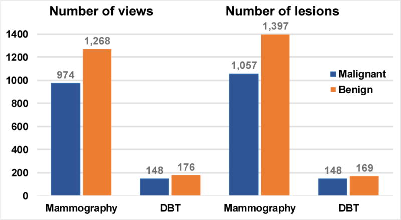
Data set characteristics. The number of views consists of craniocaudal (CC) and mediolateral (MLO) views, including CC and MLO views in the mammography data sets, CC and MLO views in the DBT-UM set and MLO views in the DBT-MGH set. Note that each patient case can have a single or multiple lesions and a lesion may not be visible on all views. After data augmentation, mammography: 19,632 ROIs and DBT: 12,680 ROIs.
2.2 Transfer learning
Deep learning requires large training data sets. Collection of medical images is time consuming and costly, as medical images with pathology proven disease are not as abundant as daily life images such as those used for ImageNet and labeling the lesion on an image often requires clinicians’ expertise. Training a DCNN for a task in medical imaging primarily relies on transfer learning for both supervised and unsupervised approaches. Because DCNNs are hierarchical representation of several feature extractors, it is assumed that transfer of such sets with some fine tuning for the target task would be robust.
We propose a multi-stage transfer learning approach; transfer learning from ImageNet-trained DCNN to mammography is performed in stage 1, and transfer learning from mammography-trained DCNN to DBT is performed in stage 2. The motivation for stage 1 transfer learning is twofold: (a) our previous work on classification of malignant and benign masses in mammograms (Samala et al., 2017) shows that transfer learning by freezing the first convolutional layer of AlexNet yielded the best performance and (b) in the same work, the multi-task approach (training on SFM and DM) versus single-task approach (training on SFM only) improved the performance. The stage 2 transfer learning is motivated by our previous work on detection of masses in mammograms (Samala et al., 2016) that showed a DCNN trained on mammograms, without additional fine-tuning, could detect masses in DBT with an average sensitivity of approximately 80%. This shows a strong similarity of the low-level features learned by the DCNN between masses in mammography and DBT. This characteristic of DCNN can be exploited by fine-tuning only a small set of deeper layer features (e.g., the last fully connected layer) with the small available DBT set to the specific task of differentiating malignant and benign masses in DBT.
In this study, for the first stage of transfer learning, we froze only the first convolutional layer and the remaining layers were allowed to update using the mammography training set. Two additional fully connected layers, F4 and F5 with 100 and 2 nodes were added to the DCNN for fine tuning towards classification of malignant and benign masses as shown in fig. 1. After this fine tuning, all the weights in the convolutional layers were frozen. In the second stage, (a) 1000 features were extracted from the F3 layer and feature selection was performed using a recursive feature elimination (Ambroise and McLachlan, 2002) strategy and (b) based on the selected N features, pruning of the DCNN was performed using genetic algorithm. The area under the receiver-operating characteristic (ROC) curve (AUC) for a random forest classifier was used to guide the feature selection from the DBT training set using a leave-one-case-out cross-validation (LOOCV) resampling method. For this purpose, each ROI input to the DCNN was propagated to the random forest classifier to generate an output score. The scores of the eight augmented samples from an original ROI were averaged to obtain a single score for that ROI. The set of average scores was then used to estimate an “ROI-based” ROC curve and its AUC value.
2.3 Layered pathway evolution with genetic algorithm
In the genetic algorithm (Goldberg, 1989), the genes in each chromosome in the population are encoded as a string of bits of 0’s or 1’s, with the length of the chromosome chosen to be the total number of nodes (or filter kernels) in the convolutional layers. The status of the nodes is indicated by a single bit of 0 or 1 for inactive or active status, respectively. Dropping nodes from the structure during DCNN training is called ‘dropout’ and many studies have shown that dropout improves the generalization ability of DCNNs. However, in this work, dropout is performed on the DCNN structure through the evolutionary method without retraining the DCNN. This is the key difference between our proposed method and previous DCNN pruning methods. The lack of retraining allows for a faster pruning. Evolution of the population is controlled by selection, crossover, and mutation. Selection of the individuals from the population is determined by maximization of the fitness values. A tournament selection method (Miller and Goldberg, 1995) selects the next generation of population by maximizing the classification accuracy in terms of AUC of the random forest classifier. A count-preserving crossover and mutation technique,(Umbarkar and Sheth, 2015; Hartley and Konstam, 1993) where the number of active bits is constrained to be a constant, guides the convergence (crossover) and divergence (mutation) towards an optimal solution. An iterative layered approach is followed for pruning the DCNN. At the first iteration, evolution of C1 layer is performed while all the layers from C2 to C5 are activated (‘1’). In the second iteration, the pruned C1 is frozen, evolution of C2 is performed while all the nodes from C3-C5 are activated. The process is repeated until the C1-C4 layers have been pruned and frozen while the evolution of C5 layer is performed.
There are 64, 192, 384, 256 and 256 nodes in the convolutional layers from C1 to C5. An individual chromosome is encoded with a string of 1152 bits representing the total number of nodes from all convolutional layers. The initial population size is 500 and every new generation has a population size of 100. In the tournament selection process, an individual with the best fitness value is selected from a group of 10 individuals (fixed tournament size) that are randomly selected from each generation. The number of active nodes in each pruned convolutional layer is chosen to be 16 to facilitate parallel implementation that adheres with graphics processing unit (GPU) memory grid design.
3. RESULTS AND DISCUSSION
The results of network pruning are shown in Table 1 and 2. There is 87% reduction in the number of neurons and 34% reduction in the number of parameters in the pruned DCNN. The number of multiply-and-add operations in the convolutional layers reduced by 95%. The total number of connections between the convolutional nodes reduced from 249,856 to 1024. Fig. 3 shows the trend of AUC as the DCNN evolved through the generations at each layered pruning stages. The iteration at which convergence of the genetic algorithm occurs depends on many factors such as initial solution by the initial population which is randomly generated and the crossover and mutation rates in the tournament selection of chromosomes. Fig. 4 shows the filter kernels from the first convolutional layer (C1) for the original DCNN with 64 nodes for the task of classifying malignant and benign breast masses and the pruned DCNN with 16 nodes. Note that the C1 layer is frozen in the first stage of transfer learning so that these kernels are the same as those in the ImageNet.
Table 1.
DCNN structure properties before and after pruning.
| Layer | Num. of Neurons | Num. of Nodes (filter size) | Num. of Parameters |
|---|---|---|---|
| Before pruning | |||
| C1 | 61,504 | 64 (11 × 11) | 23,296 |
| C2 | 43,200 | 192 (5 × 5) | 307,392 |
| C3 | 18,816 | 384 (3 × 3) | 663,936 |
| C4 | 12,544 | 256 (3 × 3) | 884,992 |
| C5 | 12,544 | 256 (3 × 3) | 590,080 |
| F1 | 4096 | 9,441,280 | |
| F2 | 4096 | 16,781,312 | |
| F3 | 1000 | 4,097,000 | |
| F4 | 100 | 100,100 | |
| F5 | 2 | 202 | |
| Total | 148,608 |
Convolutional: 1,152 Fully-connected: 9,294 |
32,889,590 |
| After pruning | |||
| C1 | 15,376 | 16 (11 × 11) | 5,824 |
| C2 | 1,350 | 16 (5 × 5) | 6,416 |
| C3 | 786 | 16 (3 × 3) | 2,320 |
| C4 | 786 | 16 (3 × 3) | 2,320 |
| C5 | 786 | 16 (3 × 3) | 2,320 |
| F1 | 4096 | 593,920 | |
| F2 | 4096 | 16,781,312 | |
| F3 | 1000 | 4,097,000 | |
| F4 | 100 | 100,100 | |
| F5 | 2 | 202 | |
| Total | 19,084 |
Convolutional: 80 Fully connected: 9,294 |
21,591,734 |
| Decrease in number of neurons: 87.2% | Decrease in number of parameters: 34.4% | ||
Table 2.
Number of multiply-and-add (MAC) computations in the convolutional layers.
| Layer | Num. of MAC operations | |
|---|---|---|
| Before pruning | After pruning | |
| C1 | 20,908,800 | 5,227,200 |
| C2 | 44,236,800 | 921,600 |
| C3 | 23,887,872 | 82,944 |
| C4 | 31,850,496 | 82,944 |
| C5 | 21,233,664 | 82,944 |
| Total | 1,42,117,632 | 6,397,632 |
| Decrease in number of MAC computations: 95.5% | ||
Fig. 3.

Layered pathway evolution using genetic algorithm. The table at the top shows the number of initial active nodes of the AlexNet (leftmost) from C1 to C5 (top to bottom) and the number of active nodes at each step of pruning in the convolutional layers. The corresponding population evolution in each convolutional layer is shown in the graph below. Five parallel bars at the top indicate the five convolutional layers either pruning, frozen or pruned. The ROI-based validation AUCs from the LOOCV resampling method are shown.
Fig. 4.
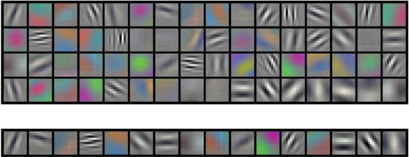
Filter kernels of size 11 × 11 pixels from convolutional layer, C1. Top: 64 nodes from original DCNN, bottom: 16 nodes from pruned DCNN. C1 layer is frozen during the first stage of transfer learning.
An independent DBT test set is used to validate the DCNN pruning method. The original DCNN, feature extraction, use of selected features (N=240) from recursive feature selection and the random forest classifier is compared with the pruned DCNN, feature extraction, use of the selected features and random forest classifier. The fitted binormal ROC curves (Metz et al., 1998) for the two approaches is shown in fig. 5 and the AUC of the original DCNN and pruned DCNN methods are 0.88±0.05 and 0.90±0.04, respectively. The difference between the two methods did not reach statistical significance (two tailed p-value > 0.05). The performance did not decrease when the DCNN structure was pruned for classification of masses in DBT and the sensitivity of the pruned DCNN were substantially higher over a wide range of specificity (i.e., 1- false positive fraction).
Fig. 5.

ROC curves for independent DBT test between original DCNN and pruned DCNN.
There are limitations in our study. We did not prune the fully connected layers and instead we chose to reduce only the number of convolutional layer nodes. For our target task of classification of masses in DBT, we chose to use the DCNN as feature extractor and hence did not need to prune the fully connected layers. However, due to the reduction in the number of filter kernels (nodes) in the C5 layer, the number of parameters in the F1 layer reduced by 93.7%, thus reducing the number of parameters for the entire fully connected layers by 29%. We did not try our pruning approach on much larger and deeper CNN structures like VGG and GoogLeNet. These other larger structures require much larger data sets for transfer training and validation, which is beyond the data set sizes that we can collect. Medical data collection is an expensive and time-consuming process that requires expert annotations for any meaningful training of computer-assisted systems. Features from DCNN can be extracted at any fully connected layers, but we chose F3 with 1000 nodes. The decision was based on the discriminability of features into malignant and benign. F1 features are less specific and more generic to target task while F5 features are more specific and less generic. F3 is a good balance but future work is needed to investigate the characteristics of the features in the different layers.
4. CONCLUSION
Transfer learning has been a valuable tool for medical imaging to overcome the limitation of data requirements to train a DCNN. In this work we propose a method to prune a large two-stage transfer learned DCNN by reducing 87% of the number of neurons, 34% of the number of parameters, and 95% of the number of multiply-and-add operations required in the convolutional layers for a classification task in DBT without a reduction in performance. Our method simulated dropout in a trained DCNN using evolutionary methods guided by diagnostic performance. The advantage of a pruned DCNN is that it requires much less memory and computations for processing an unknown image so that the efficiency increases in a high throughput environment. The validation results on the independent test set indicate potential deployment of deep learning systems into clinical workflow without excessive hardware requirements.
Acknowledgments
This work is supported by National Institutes of Health award numbers R01 CA151443 and R01 CA214981.
References
- US FOOD & DRUG ADMINISTRATION: MQSA National Statistics. 2017 Link: www.fda.gov/Radiation-EmittingProducts/MammographyQualityStandardsActandProgram/FacilityScorecard/ucm113858.htm (accessed on: 07/03/2017)
- Ambroise C, McLachlan GJ. Selection bias in gene extraction on the basis of microarray gene-expression data. Proceedings of the national academy of sciences. 2002;99:6562–6. doi: 10.1073/pnas.102102699. [DOI] [PMC free article] [PubMed] [Google Scholar]
- Anwar S, Hwang K, Sung W. Structured pruning of deep convolutional neural networks. ACM Journal on Emerging Technologies in Computing Systems (JETC) 2017;13:32. [Google Scholar]
- Chan H-P, Lo SC, Helvie M, Goodsitt MM, Cheng SNC, Adler DD. Recognition of mammographic microcalcifications with artificial neural network. Radiology. 1993;189(P):318. [Google Scholar]
- Chan H-P, Lo SCB, Sahiner B, Lam KL, Helvie MA. Computer-aided detection of mammographic microcalcifications: Pattern recognition with an artificial neural network. Medical Physics. 1995;22:1555–67. doi: 10.1118/1.597428. [DOI] [PubMed] [Google Scholar]
- Chan H-P, Sahiner B, Lo SC, Helvie M, Petrick N, Adler DD, Goodsitt MM. Computer-aided diagnosis in mammography: detection of masses by artificial neural network. Medical Physics. 1994;21:875–6. [Google Scholar]
- Dai X, Yin H, Jha NK. NeST: A Neural Network Synthesis Tool Based on a Grow-and-Prune Paradigm. arXiv preprint arXiv:1711.02017 2017 [Google Scholar]
- Dong X, Chen S, Pan SJ. Learning to Prune Deep Neural Networks via Layer-wise Optimal Brain Surgeon. arXiv preprint arXiv:1705.07565 2017 [Google Scholar]
- Fernando C, Banarse D, Blundell C, Zwols Y, Ha D, Rusu AA, Pritzel A, Wierstra D. Pathnet: Evolution channels gradient descent in super neural networks. arXiv:1701.08734 2017 [Google Scholar]
- Goldberg DE. Genetic algorithms in search, optimization, and machine learning. New York: Addison-Wesley; 1989. [Google Scholar]
- Hardesty LA, Kreidler SM, Glueck DH. Digital breast tomosynthesis utilization in the United States: a survey of physician members of the Society of Breast Imaging. Journal of the American College of Radiology. 2014;11:594–9. doi: 10.1016/j.jacr.2013.11.025. [DOI] [PubMed] [Google Scholar]
- Hartley SJ, Konstam AH. Proceedings of the 1993 ACM Conference on Computer Science. ACM; 1993. Using genetic algorithms to generate Steiner triple systems; pp. 366–71. [Google Scholar]
- Hassibi B, Stork DG, Wolff GJ. Optimal brain surgeon and general network pruning. Neural Networks, 1993, IEEE International Conference on: IEEE. 1993:293–9. [Google Scholar]
- Krizhevsky A, Sutskever I, Hinton GE. Imagenet classification with deep convolutional neural networks. Advances in Neural Information Processing Systems. 2012:1097–105. [Google Scholar]
- Li H, Kadav A, Durdanovic I, Samet H, Graf HP. Pruning filters for efficient convnets. arXiv preprint arXiv:1608.08710 2016 [Google Scholar]
- Litjens G, Kooi T, Bejnordi BE, Setio AAA, Ciompi F, Ghafoorian M, van der Laak JA, van Ginneken B, Sánchez CI. A survey on deep learning in medical image analysis. arXiv preprint arXiv:1702.05747. 2017 doi: 10.1016/j.media.2017.07.005. [DOI] [PubMed] [Google Scholar]
- Lo SC, Lin JS, Freedman MT, Mun SK. Proceedings of the SPIE-Medical Imaging 1898. 1993. Computer-assisted diagnosis of lung nodule detection using artificial convolution neural network; pp. 859–69. [Google Scholar]
- Lo SCB, Chan H-P, Lin JS, Li H, Freedman M, Mun SK. Artificial Convolution neural network for medical image pattern recognition. Neural Networks. 1995;8:1201–14. [Google Scholar]
- Metz CE, Herman BA, Shen JH. Maximum-likelihood estimation of receiver operating characteristic (ROC) curves from continuously-distributed data. Statistics in Medicine. 1998;17:1033–53. doi: 10.1002/(sici)1097-0258(19980515)17:9<1033::aid-sim784>3.0.co;2-z. [DOI] [PubMed] [Google Scholar]
- Miller BL, Goldberg DE. Genetic algorithms, tournament selection, and the effects of noise. Complex Systems. 1995;9:193–212. [Google Scholar]
- Sahiner B, Chan H-P, Petrick N, Wei D, Helvie MA, Adler DD, Goodsitt MM. Classification of mass and normal breast tissue: A convolution neural network classifier with spatial domain and texture images. IEEE Transactions on Medical Imaging. 1996;15:598–610. doi: 10.1109/42.538937. [DOI] [PubMed] [Google Scholar]
- Samala RK, Chan H-P, Hadjiiski LM, Helvie MA, Cha K, Richter C. Multi-task transfer learning deep convolutional neural network: application to computer-aided diagnosis of breast cancer on mammograms. Physics in Medicine and Biology. 2017;62:8894–908. doi: 10.1088/1361-6560/aa93d4. [DOI] [PMC free article] [PubMed] [Google Scholar]
- Samala RK, Chan H-P, Hadjiiski L, Helvie MA, Wei J, Cha K. Mass detection in digital breast tomosynthesis: Deep convolutional neural network with transfer learning from mammography. Medical Physics. 2016;43:6654–66. doi: 10.1118/1.4967345. [DOI] [PMC free article] [PubMed] [Google Scholar]
- Umbarkar A, Sheth P. Crossover operators in genetic algorithms: a review. Journal on Soft Computing. 2015;6:1083–92. [Google Scholar]