Assessing the performance of the generalized propensity score for estimating the effect of quantitative or continuous exposures on binary outcomes

Abstract

Propensity score methods are increasingly being used to estimate the effects of treatments and exposures when using observational data. The propensity score was initially developed for use with binary exposures. The generalized propensity score (GPS) is an extension of the propensity score for use with quantitative or continuous exposures (eg, dose or quantity of medication, income, or years of education). We used Monte Carlo simulations to examine the performance of different methods of using the GPS to estimate the effect of continuous exposures on binary outcomes. We examined covariate adjustment using the GPS and weighting using weights based on the inverse of the GPS. We examined both the use of ordinary least squares to estimate the propensity function and the use of the covariate balancing propensity score algorithm. The use of methods based on the GPS was compared with the use of G‐computation. All methods resulted in essentially unbiased estimation of the population dose‐response function. However, GPS‐based weighting tended to result in estimates that displayed greater variability and had higher mean squared error when the magnitude of confounding was strong. Of the methods based on the GPS, covariate adjustment using the GPS tended to result in estimates with lower variability and mean squared error when the magnitude of confounding was strong. We illustrate the application of these methods by estimating the effect of average neighborhood income on the probability of death within 1 year of hospitalization for an acute myocardial infarction.

1. INTRODUCTION

In many observational studies, the treatment or exposure variable may not be binary, but categorical or continuous. When the exposure is continuous, the objective is the estimation of a dose‐response function, relating the value of the exposure variable to the mean or expected outcome. In conducting such studies, analysts must account for the confounding that occurs when the distribution of baseline covariates differs between treated and control subjects. Appropriate statistical methods must be used to account for this confounding so that valid inferences on treatment effects can be drawn from observational studies. Statistical methods based on the propensity score are increasingly being used to reduce or minimize the confounding that occurs in observational studies.1, 2

The propensity score was developed by Rosenbaum and Rubin for use with binary or dichotomous treatments or exposures (eg, active treatment vs control). However, propensity score methods have subsequently been extended to allow analysts to estimate the effect of continuous or quantitative exposures.3, 4, 5 Examples of such quantitative exposures include dose or quantity of medication used, pack‐years of cigarettes smoked, income, or years of education. The extension of propensity score methods to quantitative exposures has been referred to as the generalized propensity score (GPS).5, 6

The original methods papers that introduced the GPS considered continuous outcomes such as labor earnings,5, 6 medical expenditures,4 and birth weight.7 In biomedical research, binary or dichotomous outcomes occur frequently (eg, death vs survival and presence vs absence of complications after surgery).8 Despite the frequency of binary outcomes and the increased use of the GPS, there is a paucity of studies examining the performance of the GPS for estimating the effect of continuous or quantitative exposures on binary outcomes.

The objective of the current study was to examine the performance of different methods when using the GPS to estimate the effect of continuous or quantitative exposures on binary outcomes. The paper is structured as follows: In Section 2, we provide notation, a brief background on the GPS, and describe methods for using the GPS to estimate the effect of continuous exposures on binary outcomes. In Section 3, we use Monte Carlo simulations to evaluate the performance of these methods. In Section 4, we provide a case study to illustrate estimation of the effect of average neighborhood income on the probability of death within 1 year of hospital admission using a sample of patients hospitalized with acute myocardial infarction (AMI). Finally, in Section 5, we summarize our findings and place them in the context of the existing literature.

2. USING THE GPS WITH BINARY OUTCOMES

In this section, we introduce the GPS. We then describe 2 ways, in which it can be used to estimate the dose‐response function for a quantitative exposure and binary outcomes.

2.1. Notation and assumptions

We use the following notation throughout the paper. Let T denote a continuous or quantitative variable denoting the level of exposure (eg, dose or quantity of a medication), and let X denote a vector of measured baseline covariates. We work within Rubin's potential outcomes framework for causal inference.9 This assumes the existence of a set of potential outcomes, Y_i(t), for t ∈ Ψ. Y_i(t) denotes the outcome of the ith subject if they received exposure T = t, while Ψ denotes the set of all possible values of the exposure. In the conventional setting with a dichotomous exposure, Ψ = {0, 1}. When using the GPS with quantitative exposures, Ψ is a subset of the real line (Ψ ⊂ ℜ).

We make the stable unit treatment value assumption, which posits that Y_i(t), the response by the ith subject under exposure T = t, is not affected by how treatment was assigned or by what exposures are received by other subjects.10, 11 Finally, we require the weak unconfoundedness assumption: Y(t) ⊥ T ∣ X for all t ∈ Ψ.5

2.2. The GPS

Using the terminology of Hirano and Imbens, let r(t, x) denote the conditional density of the continuous exposure variable given the covariates:

$$r\left(t,x\right)=f_{T\mid X}\left(t|x\right).$$ (1)

Then the GPS is R = r (T, X).5 Imai and van Dyk refer to the conditional density function f _T|X as the propensity function.4 The propensity function can be estimated by regressing the quantitative outcome on the set of observed baseline covariates. In practice, this might be done using ordinary least squares (OLS) regression. When using OLS regression, one can determine the density function of the conditional distribution of the continuous exposure by using the estimated regression coefficients and the estimated residual variance. For a given subject, the density function can be evaluated at the observed value of that subject's exposure. This is the value of the GPS for that subject.

The GPS is a balancing function: X ⊥ 1{T = t} ∣ r (t, X).5 Thus, the probability that T = t is independent of X. This is similar to the balancing property of the conventional propensity score for use with binary treatments, which states that the distribution of observed covariates is the same between treated and control subjects who share the same value of the propensity score.1

While OLS regression may be the most common method of estimating the propensity function, other methods have been suggested. Imai and Ratkovic described the covariate balancing propensity score (CBPS) methodology, which models treatment assignment while optimizing covariate balance.12 Fong et al subsequently extended the CBPS methodology to quantitative exposures.13 Both Flores et al and Bia et al suggested using that generalized linear models could be used to estimate the propensity score function.14, 15

2.3. Estimation of the dose‐response function using the GPS

The dose‐response function is defined as μ (t) = E[Y_i(t)]. This dose‐response function denotes the average response in the population (or sample) if all subjects were to receive T = t. By comparing μ(t₁) with μ(t₂), one can estimate the mean change in the outcome if all subjects were exposed with T = t₂ instead of T = t₁. A variety of methods have been proposed for using the GPS to estimate the dose‐response function.3, 5, 6, 7, 16 We will focus on 2 approaches: covariate adjustment using the GPS and weighting using the inverse of the GPS. When outcomes are binary, the dose‐response function relates the value of the continuous or quantitative exposure to the probability of the occurrence of the outcome.

When using covariate adjustment using the GPS, one regresses the occurrence of the binary outcome on the continuous treatment and the estimated GPS using logistic regression.5, 6 Based on the fitted regression model, one can then estimate the probability of the occurrence of the outcome for a given subject if their exposure was set equal to T = t. By taking the mean of this quantity over the study sample, one can estimate the dose‐response function: μ(t) = E[Y_i(t)].

Both Imbens and Robins et al suggested that weights could be derived from the GPS. These weights can then be used to estimate the dose‐response function.3, 7 Weights can be defined as $\frac{W\left(T_i\right)}{r\left(T_i|X_i\right)}$, where the numerator is a function of T that is included to stabilize the weights. It has been suggested that a reasonable choice for W is an estimate of the marginal density function of T.7 Note that the denominator of a given weight is the value of the density function for a conditional normal distribution evaluated at the observed exposure level. Subjects with exposure levels closer to the conditional mean (and thus more “typical”) will have a greater value for the density function and will have a correspondingly lower weight. Conversely, subjects with exposure levels further from the conditional mean (and thus less “typical”) will have a smaller value for the density function and will have a correspondingly greater weight. Once the GPS‐based weights have been estimated, a univariate logistic regression can be conducted, in which the occurrence of the outcome is regressed on the continuous exposure using a weighted regression model that incorporates the GPS‐based weights. From the fitted outcomes model, the dose‐response function can be estimated by calculating the mean probability of the occurrence of the outcome across all levels of exposure.

Alternative methods to estimating the dose‐response function have been described recently. Both Flores et al and Bia et al suggest that kernel methods and penalized spline methods can be used to estimate the dose‐response function.14, 15

3. MONTE CARLO SIMULATIONS OF THE PERFORMANCE OF THE GPS FOR ESTIMATING THE EFFECT OF CONTINUOUS EXPOSURES ON BINARY OUTCOMES

We conducted a series of Monte Carlo simulations to examine the performance of different methods of using the GPS to estimate the effect of continuous exposures on binary outcomes.

3.1. Methods

3.1.1. Simulating a large superpopulation

We simulated baseline covariates and a continuous exposure for a large population consisting of 1 000 000 subjects. Ten baseline covariates (X₁ − X₁₀) were simulated for each subject from independent standard normal distributions. For each subject, a continuous exposure variable was generated from the following linear model:

$$T_i=1x_{1i}+1.5x_{2i}+2x_{3i}+3x_{4i}-2x_{5i}-2x_{6i}+1x_{7i}+1.5x_{8i}+2x_{9i}+3x_{10i}+{\epsilon }_i,$$ (1)

where ε_i~N(0, σ²). Thus, increasing values of 8 of the baseline variables were associated with an increase in the mean exposure, while increasing values of 2 of the variables were associated with a decrease in the mean exposure. The value of σ² was chosen so that variation in the 10 baseline covariates would explain a desired proportion of the variation in the continuous exposure (see below). Note that the intercept in the above model is equal to zero. Without loss of generality, we simulated data so that for a subject whose covariates are all equal to zero, the mean exposure is equal to zero.

We then determined the probability of the occurrence of the binary outcome for each subject using the following logistic model:

$$\begin{array}{l}\text{logit}\left(p_i\right)=log\left(2\right)x_{1i}+log\left(3\right)x_{2i}+log\left(0.25\right)x_{3i}+log\left(0.33\right)x_{4i}+log\left(0.5\right)x_{5i}+log\left(1.5\right)x_{6i}+\\ log\left(2\right)x_{7i}+log\left(0.5\right)x_{8i}+log\left(0.5\right)x_{9i}+log\left(2\right)x_{10i}+log\left(1.5\right)t_i,\end{array}$$ (2)

where p _i denotes the probability of the occurrence of the binary outcome. We simulated a binary outcome for each subject from a Bernoulli distribution with subject‐specific parameter p _i: Y_i~Be(p_ij). Thus, increasing values of 5 of the covariates were associated with an increase in the odds of the occurrence of the outcome, while increasing values of 5 of the covariates were associated with a decrease in the odds of the occurrence of the outcome. Increasing values of the continuous exposure were associated with an increase in the odds of the occurrence of the outcome. The intercept in the above model is equal to zero, so that the probability of the occurrence of the outcome is equal to 0.5 for a subject whose covariates are equal to zero and for whom the exposure is also equal to zero.

We then determined the population dose‐response function at a predetermined number of values of the continuous exposure variable. We computed the 9 deciles of the population distribution of the continuous exposure. We refer to these 9 deciles as the 9 exposure thresholds and denote these exposure thresholds by T  ^k, k = 1, …, 9. We then simulated an outcome for each subject in the large superpopulation if everyone in the superpopulation had their exposure set equal to the first of the 9 exposure threshold values:

$$\begin{array}{l}{Y}_i^k~\mathrm{Be}\left(p_i^k\right),\text{where}\\ \text{logit}\left(p_i^k\right)=log\left(2\right)x_{1i}+log\left(3\right)x_{2i}+log\left(0.25\right)x_{3i}+log\left(0.33\right)x_{4i}+log\left(0.5\right)x_{5i}+log\left(1.5\right)x_{6i}+\\ log\left(2\right)x_{7i}+log\left(0.5\right)x_{8i}+log\left(0.5\right)x_{9i}+log\left(2\right)x_{10i}+log\left(1.5\right)T^k\\ \text{for}k=1,\dots ,9.\end{array}$$ (3)

The difference between Formulas (2) and (3) is that in the latter formula, rather than using the simulated exposure level, we fix the exposure level at a given exposure threshold. We then determined the probability of the occurrence of the outcome across the superpopulation. This was computed as the mean of simulated outcome variable when all subjects had their value of the continuous exposure set equal to the first of the 9 exposure thresholds. This process was repeated for the other 8 exposure thresholds values. These 9 values will serve as the values of the population dose‐response function. Thus, we have that

$$\mu \left(T^k\right)=\frac{1}{N}\sum _{i=1}^N{Y}_i^k,\text{for}k=1,\dots ,9.$$ (4)

In our simulations, the population dose‐response function consisted of 9 pairs of numbers. The first member of each pair consisted of 1 of the 9 deciles of the distribution of the continuous exposure, while the second member of each pair consisted of the marginal probability of the outcome if all members of the population were to receive that level of exposure. We note that the true dose‐response function is a function that can be evaluated at all values of a subset of the real line. However, to evaluate the performance of different methods of using the GPS to estimate the dose‐response function with binary outcomes, we are required to evaluate the dose‐response function at a finite number of points. This will permit summarizing performance using bias, variance, and mean squared error (MSE). We elected to evaluate the dose‐response function at the 9 deciles of the exposure variable, as this permits assessment of performance across a wide range of plausible values of the exposure.

3.1.2. Monte Carlo simulations

From the large superpopulation, we drew a random sample of 1000 subjects. In this random sample, we estimated the propensity function using 2 different methods. First, we used OLS regression to regress the observed continuous exposure variable on all 10 measured baseline covariates:

$$T_i=a_0+a_1{x}_{1i}+a_2{x}_{2i}+a_3{x}_{3i}+a_4{x}_{4i}+a_5{x}_{5i}+a_6{x}_{6i}+a_7{x}_{7i}+a_8{x}_{8i}+a_9{x}_{9i}+a_{10}{x}_{10i}+{\epsilon }_i,\text{where}{\epsilon }_i~N\left(0,{\sigma }^2\right).$$

The GPS was estimated under the assumption that the conditional distribution of the exposure was normal with mean equal to the linear predictor and with variance equal to the residual variance of the fitted OLS regression model. For a given subject, let ${\widehat{\alpha }}^t\mathbf{X}$ denote the mean exposure level on the basis of the above regression model. Similarly, let $\widehat{\sigma }$ denote the estimated standard deviation of the residuals. Then f_{T ∣ X}(t| x) can be estimated by the normal density function $\frac{1}{\sqrt{2\pi {\widehat{\sigma }}^2}}{e}^{-\frac{{\left(t-{\widehat{\mathbf{\beta }}}^t\mathbf{X}\right)}^2}{2{\widehat{\sigma }}^2}}$.

Second, we used the CBPS method to estimate the propensity function by regressing the observed continuous exposure variable on all 10 measured baseline covariates. We refer to the 2 different estimates of the GPS as GPS‐OLS and GPS‐CBPS to indicate the method used to estimate the propensity function.

We then used the 2 methods described above for using the GPS to estimate the dose‐response function for binary outcomes. When using GPS‐based weights, we used the stabilized weights recommended by Robins et al, in which the numerator was based on the marginal density of the continuous exposure variable. This density function can be determined by calculating the mean and the standard deviation of the quantitative exposure variable in the overall sample (μ_sample and σ_sample, respectively). Then $W\left(T_i\right)=\frac{1}{\sqrt{2{\mathit{\pi \sigma }}_{\text{sample}}^2}}{e}^{-\frac{{\left(T_i-{\mu }_{\text{sample}}\right)}^2}{2{\sigma }_{\text{sample}}^2}}$.17 Robins et al note that for quantitative exposures, unstabilized weights (ie, those with W(T _i) = 1) will have infinite variance and should not be used.17 We estimated the dose‐response function at the 9 exposure threshold described above (the 9 deciles of the population distribution of the continuous exposure).

For comparative purposes, we also examined the performance of G‐computation.18 G‐computation requires that an outcomes model be fit to the data, in which the outcome is regressed on baseline covariates and the exposure variable. The fitted regression model is then used to impute or estimate potential outcomes under different treatment conditions. As such, it assumes that the outcomes regression model has been correctly specified. In each of the random samples, we did the following:

• 1We used logistic regression to regress the occurrence of the binary outcome on the continuous exposure variable and the 10 baseline covariates:

logit(p_i) = b₀ + b₁x_1i + b₂x_2i + b₃x_3i + b₄x_4i + b₅x_5i + b₆x_6i + b₇x_7i + b₈x_8i + b₉x_9i + b₁₀x_10i + b₁₁t_i.

• 2We then created 9 pseudosamples that were replicas of the random sample in terms of the 10 baseline covariates. However, the pseudosamples differed in terms of the continuous exposure. In the first pseudosample, the value of the continuous exposure for all subjects was set equal to the first threshold value of the continuous exposure that was computed above. In the second pseudosample, the value of the continuous exposure for all subjects was set equal to the second threshold value of the continuous exposure that was computed above. Similar modifications were made in the other 7 pseudosamples.
• 3The fitted logistic regression model was then applied to each of these 9 pseudosamples to estimate the predicted probability of the outcome under a given treatment threshold: $\text{logit}\left(p_i^k\right)=b_0+b_1{x}_{1i}+b_2{x}_{2i}+b_3{x}_{3i}+b_4{x}_{4i}+b_5{x}_{5i}+b_6{x}_{6i}+b_7{x}_{7i}+b_8{x}_{8i}+b_9{x}_{9i}+b_{10}{x}_{10i}+b_{11}{T}^k.$
• 4Within each of the 9 pseudosamples, the mean predicted probability of the outcome was then determined: $\mu \left(T^k\right)=\frac{1}{N}\sum _{i=1}^N{p}_i^k$. These were used as estimates of the value of the dose‐response function at the 9 thresholds of the continuous exposure.

The process of drawing random samples of size 1000 from the superpopulation was conducted 10 000 times. For each estimation method, we determined the mean dose‐response function across the 10 000 iterations of the simulations. For each of the 9 exposure thresholds, we determined the standard deviation of the value of the dose‐response function across the 10 000 iterations of the simulations. Finally, using the true known value of the population dose‐response function (determined above), for each of the 9 exposure thresholds, we determined the MSE of the estimated dose‐response function across the 10 000 iterations of the simulations.

One factor was allowed to vary in the Monte Carlo simulations: the proportion of the variation in the continuous exposure that was explained by variation in the 10 baseline covariates. We considered 8 values for this R ²: 0.1, 0.2, 0.3, 0.4, 0.5, 0.6, 0.7, and 0.8. We thus constructed 8 different superpopulations. From each superpopulation, we drew 10 000 random samples and conducted the statistical analyses described above. The magnitude of the R ² statistic can be thought of as a measure of the magnitude of confounding. Higher values of R ² are indicative of a greater correlation between the continuous exposure variable and a linear combination of the baseline covariates. Thus, we considered scenarios in which the magnitude of confounding ranges from weak to very strong.

We explored the effect of these different R ² values on the degree of overlap of the distribution of the continuous exposure between subjects with different covariate patterns. Within each of the superpopulations, we computed the linear predictor for the continuous exposure for each subject (ie, the linear combination of the 10 baseline covariates). Subjects were then divided into 5 strata according to the quintiles of the linear predictor. Side‐by‐side boxplots were used to compare the distribution of the continuous exposure across these 5 strata (Figure 1). In examining Figure 1, one observes that as the R ² value increases, there is increasingly less overlap between the distribution of the continuous exposure and the different strata on the basis of the linear predictor. This highlights that by varying R ², we can examine scenarios with different degrees of overlap in the distribution of the continuous exposure between different subsets of subjects.

Figure 1.

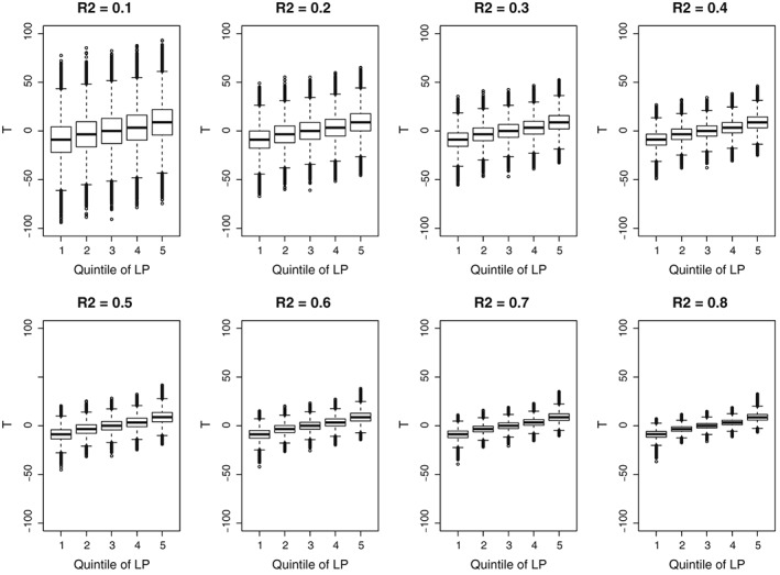
Distribution of the continuous exposure across quintiles of the linear predictor (LP)

We considered 2 additional sets of scenarios in addition to the primary set of simulations described above. First, we repeated the above simulations with the size of each simulated dataset being 500 (instead of 1000). Second, we modified the magnitude of the strength of the covariates on exposure level and on the odds of the binary outcome. In Equation (1), we doubled each of the regression coefficients, so that each covariate had a stronger effect on the exposure level. We also doubled each of the odds ratios in Equation (2), so that each covariate had a stronger effect on the odds of the occurrence of the binary outcome.

4. RESULTS

4.1.

4.1.1. Primary simulations (N = 1000)

The results of the Monte Carlo simulations for the primary set of simulations (N = 1000 and regression coefficients as in Formulas (1) and (2)) are reported in Figures 2, 3, 4. Each figure consists of 8 panels. There is one panel for each of the 8 scenarios defined by the proportion of the variation in continuous exposure variable that was explained by variation in the baseline covariates.

Figure 2.

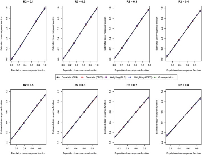
Comparison of estimated dose‐response function with population dose‐response function at the deciles of treatment (N = 1000). CBPS, covariate balancing propensity score; OLS, ordinary least squares [Colour figure can be viewed at http://wileyonlinelibrary.com]

Figure 3.

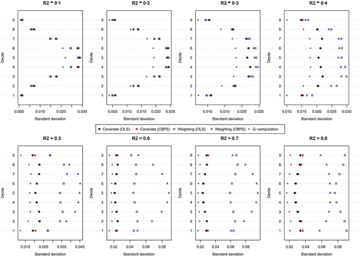
Standard deviation of estimated dose‐response function at the deciles of treatment (N = 1000). CBPS, covariate balancing propensity score; OLS, ordinary least squares [Colour figure can be viewed at http://wileyonlinelibrary.com]

Figure 4.

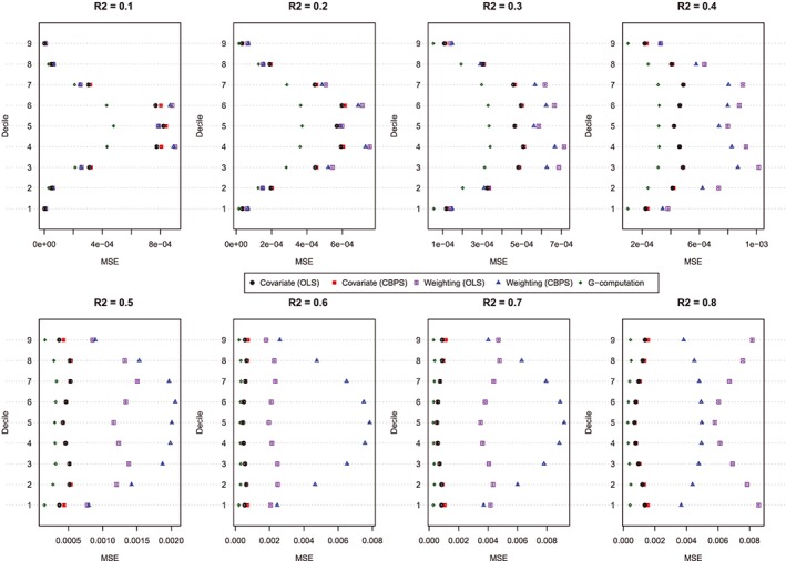
MSE of estimated dose‐response function at the deciles of treatment (N = 1000). CBPS, covariate balancing propensity score; MSE, mean squared error; OLS, ordinary least squares [Colour figure can be viewed at http://wileyonlinelibrary.com]

The mean estimated dose‐response function for each method is reported in Figure 2. In each panel, we plotted the values of the estimated dose‐response function against the values of the population dose‐response function at the 9 exposure thresholds. We have superimposed on each panel a diagonal line with slope 45°. Methods that resulted in unbiased estimation of the dose‐response function will result in estimates that lie along this diagonal line. In examining Figure 2, one observes that all methods resulted in essentially unbiased estimation of the population dose‐response function. The magnitude of confounding (as measured by the R ² statistic) had no discernible effect on the bias of the different methods. All methods performed well regardless of the magnitude of confounding.

The standard deviations of the estimated values of the dose‐response function are described in Figure 3. Each panel consists of a dot chart. Each dot chart is composed of 9 horizontal lines, 1 for each of the 9 exposure threshold values. On each of these horizontal lines are 5 symbols, denoting the standard deviation of the estimated value of the dose‐response function for the 5 estimation methods: (1) covariate adjustment using the GPS‐OLS, (2) covariate adjustment using the GPS‐CBPS, (3) weighting using GPS‐OLS‐based weights, (4) weighting using GPS‐CBPS–based weights, and (5) G‐computation. In general, G‐computation resulted in estimates that displayed the least variability. When using covariate adjustment using the GPS, there was little difference in variability of the estimated effects when OLS regression was used compared with when CBPS was used to estimate the propensity function. When the baseline covariates explained a modest proportion of the variation in the continuous exposure (R ² ≤ 0.3), then there was little difference in the variability of the estimated effects between the 2 different weighted estimators (GPS‐OLS weights and GPS‐CBPS weights). Finally, when the magnitude of confounding was strong (R ² ≥ 0.4), covariate adjustment using the GPS tended to display less variability than did GPS‐based weighting. Furthermore, when the magnitude of confounding was very strong (R ² ≥ 0.6), the method of estimating the propensity function (OLS vs CBPS) had a strong impact on the variation of the estimated effect when weighting was used.

The MSE of the estimated values of the dose‐response function is described in Figure 4. Figure 4 has a similar structure to Figure 3. In general, G‐computation resulted in estimates with the lowest MSE. Among the GPS‐based methods, covariate adjustment using the GPS tended to result in estimates with modestly lower MSE than did GPS‐based weighting. Differences between these 2 approaches were amplified as the magnitude of confounding (as measured using the R ²) increased. In general, covariate adjustment using GPS‐OLS and GPS‐CBPS resulted in estimates with similar MSE. However, when using GPS‐based weighting, the method of estimating the propensity function had a noticeable impact on the MSE of the estimated effect. However, results were inconsistent as to which of the 2 estimation methods resulted in estimates with the lowest MSE.

4.1.2. Secondary simulations

The results for the secondary simulations are reported in Figures 5, 6, 7 for the setting with N = 500. In smaller sample sizes, the observed results were qualitatively similar to those observed in the primary simulations whose results were described in detail above. When the magnitude of the effect of the covariates on the level of exposure and on the odds of the occurrence of the outcome were increased, the results of the simulations were qualitatively similar to those observed for the primary simulations (data not shown).

Figure 5.

Comparison of estimated dose‐response function with population dose‐response function at the deciles of treatment (N = 500). CBPS, covariate balancing propensity score; OLS, ordinary least squares [Colour figure can be viewed at http://wileyonlinelibrary.com]

Figure 6.

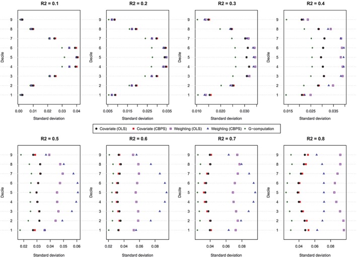
Standard deviation of estimated dose‐response function at the deciles of treatment (N = 500). CBPS, covariate balancing propensity score; OLS, ordinary least squares [Colour figure can be viewed at http://wileyonlinelibrary.com]

Figure 7.

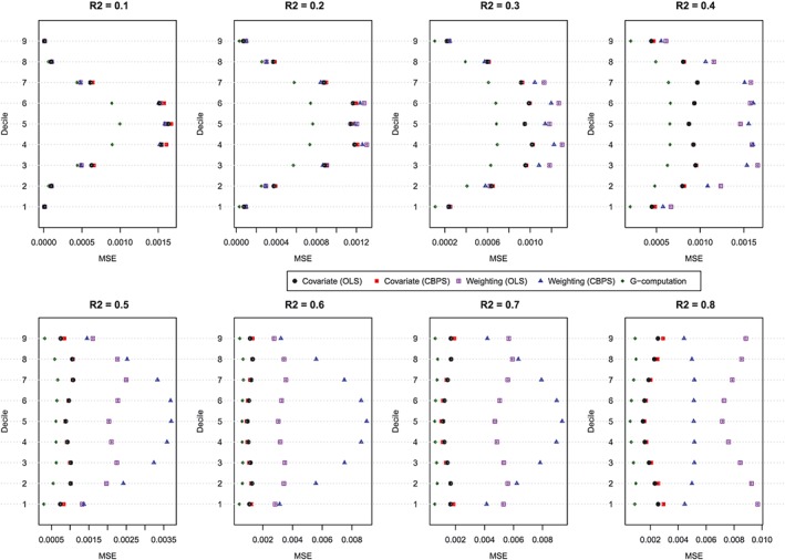
MSE of estimated dose‐response function at the deciles of treatment (N = 500). CBPS, covariate balancing propensity score; MSE, mean squared error; OLS, ordinary least squares [Colour figure can be viewed at http://wileyonlinelibrary.com]

5. CASE STUDY

We provide an empirical example to illustrate the application of the proposed methods to estimate the effect of average neighborhood income on the probability of death within 1 year of hospitalization for an AMI. In social epidemiology and health services research, there is often an interest in examining the effect of neighborhood characteristics on patient outcomes. An example in cardiovascular research is a study examining the effects of neighborhood income on access to invasive cardiac procedures and mortality after an AMI.19 An example from the endocrinology literature is a study examining the effect of neighborhood income on mortality in patients with diabetes.20

5.1. Data and analyses

We used data consisting of 10 007 patients hospitalized with an AMI in Ontario, Canada, between April 1999 and March 2001. Data on patient characteristics were obtained by retrospective chart review by trained cardiovascular research nurses. These data were collected as part of the Enhanced Feedback for Effective Cardiac Treatment Study.21 These data were linked to census data from Statistics Canada to determine the average neighborhood income for each subject (neighborhood was defined using the patient's forward sortation area, which is defined by the first 3 characters of the patient's postal code) and to the Registered Persons Database to determine the vital status of each subject. Average neighborhood income was used as the continuous exposure variable in this case study. For the purposes of regression modeling, average neighborhood income was standardized to have mean zero and unit variance. For the current case study, we considered the binary outcome denoting whether the subject died within 1 year of hospital admission.

The propensity function was estimated using 2 different methods: first, by regressing standardized average neighborhood income on a set of 34 baseline covariates using a linear regression model estimated using OLS and, second, by using the CPBS methodology to regress standardized average neighborhood income on a set of 34 baseline covariates. The 34 baseline covariates included demographic characteristics (age and sex), vital signs on admission (systolic and diastolic blood pressure, respiratory rate, and heart rate), initial laboratory values (white blood count, hemoglobin, sodium, glucose, potassium, and creatinine), signs and symptoms on presentation (acute congestive heart failure and cardiogenic shock), classic cardiac risk factors (family history of heart disease, current smoker, history of hyperlipidemia, and hypertension), and comorbid conditions (chronic congestive heart failure, diabetes, stroke or transient ischemic attack, angina, cancer, dementia, previous AMI, asthma, depression, hyperthyroidism, peptic ulcer disease, peripheral vascular disease, previous coronary revascularization, history of bleeding, renal disease, and aortic stenosis). For both OLS estimation and CBPS estimation, the effect of each continuous covariate on average neighborhood income was modeled using restricted cubic splines with 4 knots.22

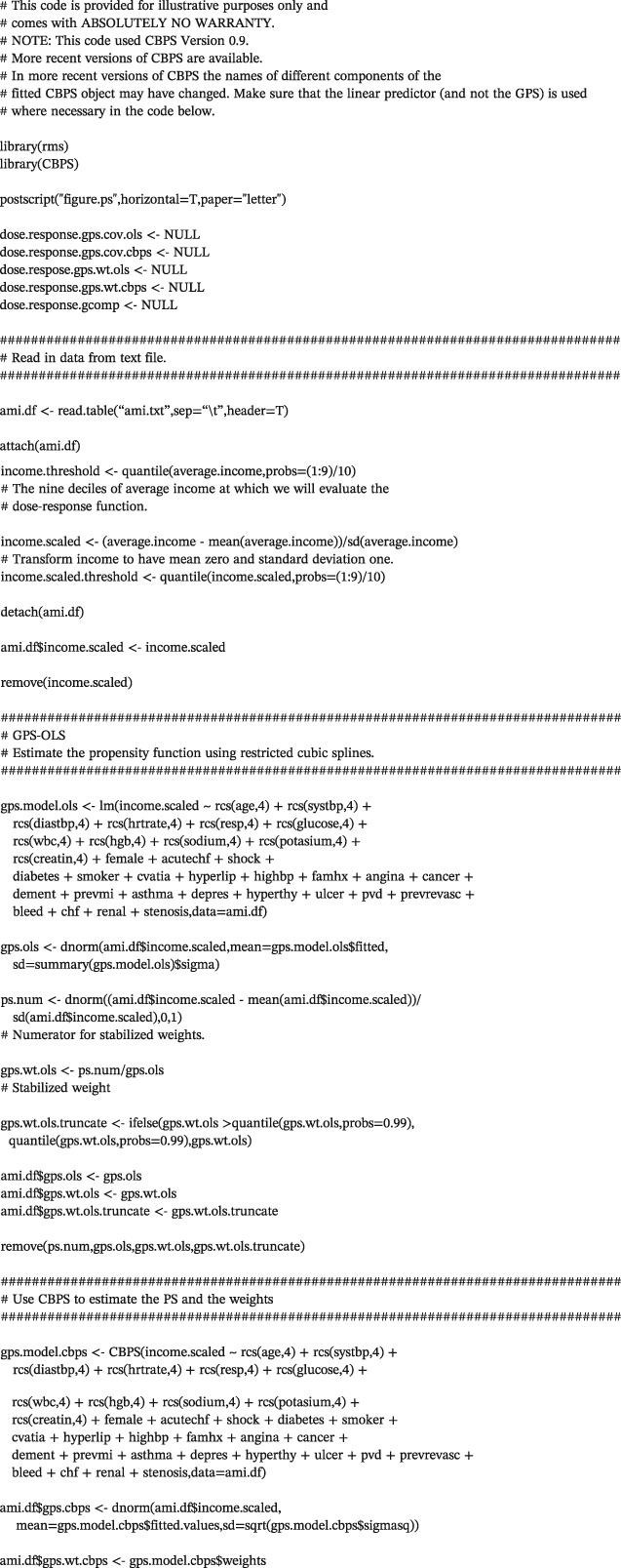
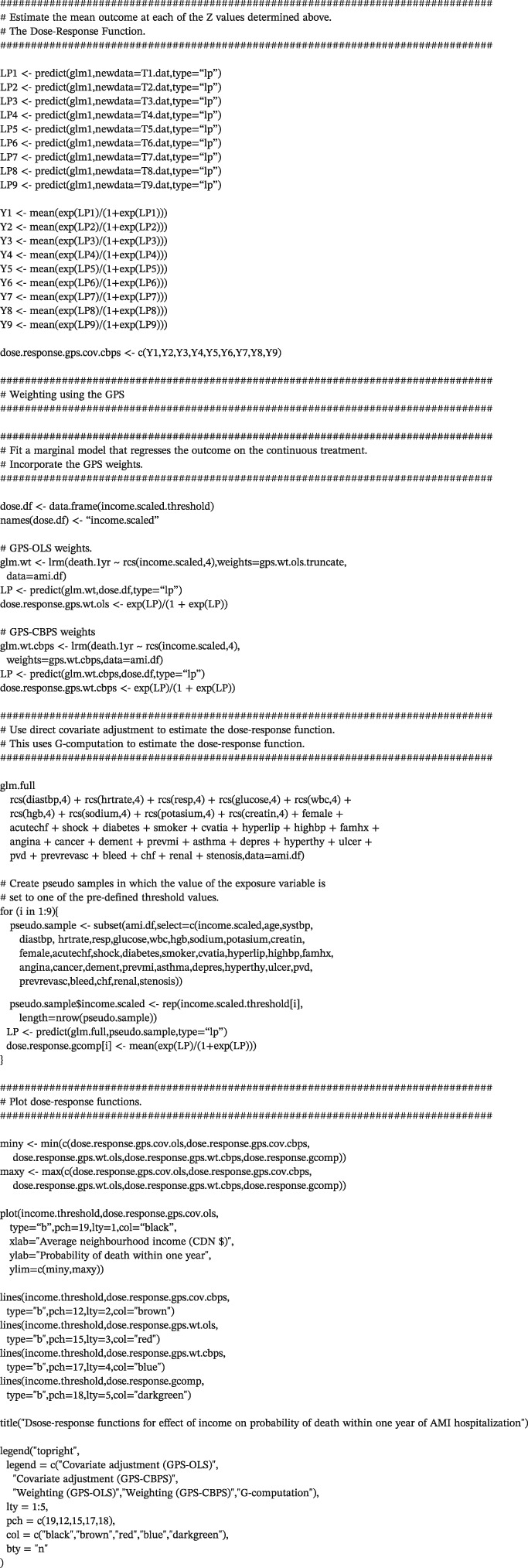
We computed the 9 deciles of the continuous exposure (average neighborhood income). We then used the methods described in Section 2, whose performance we evaluated in Section 3, to estimate the dose‐response function at these 9 deciles of average neighborhood income. When using covariate adjustment using the GPS, the occurrence of death within 1 year of hospital admission was regressed on the GPS and standardized average neighborhood income (this was done separately for both the GPS with OLS estimation and the GPS with CBPS estimation). Restricted cubic splines with 4 knots were used to model the relationship of each of these 2 covariates with the log‐odds of death. When using weighting using GPS‐based weights, truncation was used for the stabilized GPS‐OLS–based weights because of the small number of subjects with very large weights.23 Truncation was implemented by setting all weights that exceeded the 99th percentile of the distribution of weights to be equal to the 99th percentile of the distribution of weights. When fitting the weighted logistic regression in which the occurrence of death within 1 year was regressed on standardized average neighborhood income, restricted cubic splines with 4 knots were used to model the relationship between the log‐odds of death and standardized average neighborhood income. When using G‐computation, logistic regression was used to regress the occurrence of death within 1 year on standardized average neighborhood income and the 34 baseline covariates described above. In this model, the effect of each continuous covariate (including standardized average neighborhood income) was modeled using restricted cubic splines with 4 knots. Code in the R statistical programming language for conducting these analyses is described in Appendix A.

5.2. Results

The estimated dose‐response function is described in Figure 8. The figure depicts the estimated dose‐response function that describes the relationship between average neighborhood income and the probability of death within 1 year of hospitalization with an AMI. The shape of the dose‐response function was qualitatively similar across the 5 different estimation methods. The effect of average neighborhood income was more muted when using G‐computation than it was for the other 4 methods. For each of the dose‐response functions, the probability of death increased initially within increasing average neighborhood income. It reached a maximum and then began to decrease with increasing average neighborhood income. When using weighting, there was relatively little difference between the dose‐response functions obtained using weights obtained using OLS regression and weights obtained using the CBPS. Similarly, there was little difference between the approaches when using covariate adjustment using the GPS.

Figure 8.

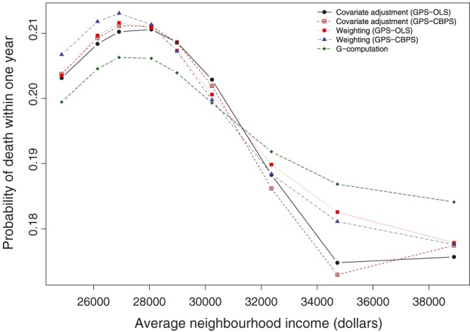
Dose‐response functions for effect of income on probability of death within 1 year of acute myocardial infarction hospitalization. CBPS, covariate balancing propensity score; GPS, generalized propensity score; OLS, ordinary least squares [Colour figure can be viewed at http://wileyonlinelibrary.com]

When using covariate adjustment using the GPS‐OLS, the difference in the probability of 1‐year mortality between the lowest and highest values of the dose‐response function was 0.036. When using CBPS to estimate the GPS, the difference in the probability of 1‐year mortality between the lowest and highest values of the dose‐response function was 0.038. For weighting using GPS‐OLS–based weights, the corresponding difference was 0.034. When using the GPS‐CBPS–based weights, the difference was 0.036. For G‐computation, the corresponding difference was 0.022.

The shape of the dose‐response function at lower values of neighborhood income is unexpected, with the probability of death within 1 year initially increasing with increasing income and then reaching a maximum and subsequently decreasing with increasing income (although note that the initial increase in the probability of mortality ranged from 0.006 to 0.008). It is possible that the analysis was affected by unmeasured confounding, in that there were unmeasured characteristics, either at the individual level or at the level of the neighborhood, such that neighborhoods with very low incomes also had characteristics that were protective for 1‐year mortality. Neighborhood characteristics that would warrant further exploration would be the location of the neighborhood (rural or urban). Subject characteristics that would warrant further exploration, but to which we do not have access would be lifestyle characteristics (exercise and diet) and ethnicity.

6. DISCUSSION

In the current study, we evaluated the performance of different methods of using the GPS to estimate the effect of continuous exposures on binary outcomes. We found that all methods resulted in essentially unbiased estimation of the underlying dose‐response function. However, the use of a weighted logistic regression using GPS‐based weights (estimated either using OLS or CBPS) tended to result in estimates that displayed greater variability and that had higher MSE than did estimates obtained using covariate adjustment using the GPS. This difference was particularly evident when the baseline covariates explained a high proportion of the variation in the continuous exposure.

As noted in Section 1, the original papers that introduced the GPS considered continuous outcomes such as labor earnings,5, 6 medical expenditures,4 and birth weight.7 In biomedical research, binary or dichotomous outcomes occur frequently.8 Despite the frequency of binary outcomes in biomedical and epidemiological research and the increased use of the GPS, there is a paucity of studies examining the performance of the GPS for estimating the effect of continuous or quantitative exposures on binary outcomes. The current study fills this gap in the existing literature.

In our simulations, we observed that GPS‐based weighting tended to result in estimates that displayed the greatest variability when the strength of confounding was strong (R ² ≥ 0.4). The reason for this high variability is likely provided by examining Figure 1. In Figure 1, it was observed that as R ² increased, the degree of overlap in the distribution of the continuous exposure between subjects with different covariate patterns decreased. We hypothesize that this may have resulted in some subjects having large weights, resulting in estimates with high variability.

In the current study, we observed that all methods resulted in estimates of the dose‐response function with minimal bias. G‐computation tended to result in estimates that displayed the lowest variability, particularly when the magnitude of confounding was strong. This suggests that G‐computation would be an attractive analytic option. However, G‐computation requires that an outcome model be specified. In practice, it is difficult to ascertain whether a multivariable outcomes model has been correctly specified. In contrast to this, a variety of balance diagnostics have been proposed for use with the GPS.5, 6, 24 These allow one to assess whether incorporating the GPS has allowed one to balance the distribution of measured baseline covariates between subjects with different values of the continuous exposure. Thus, from an implementation perspective, the use of GPS‐based methods is appealing.

There are certain limitations to the current study. The primary limitation is that the evaluation of the performance of different methods of using the GPS to estimate the effect of continuous exposures on binary outcomes was conducted using Monte Carlo simulations. For pragmatic reasons, we were constrained to examining a limited number of scenarios in our simulations. It is possible that results would differ under different data‐generating processes. However, the magnitude of the strength of confounding varied strongly across the 8 scenarios. Thus, we examined scenarios that were representative of a wide range of plausible scenarios. Furthermore, our use of simulations reflects what is frequently done to evaluate the performance of propensity score methods when used with dichotomous outcomes.25, 26, 27, 28, 29, 30, 31, 32, 33, 34, 35, 36, 37

In summary, the current study represents the first study to examine the performance of different methods of using the GPS to estimate the effect of continuous or quantitative exposures on binary outcomes. We found that both covariate adjustment using the GPS and weighting using GPS‐based weights resulted in unbiased estimation of the dose‐response function. However, weighting with GPS‐based weights tended to result in estimates of the values of the dose‐response function that displayed greater variability, particularly when the magnitude of confounding was strong.

APPENDIX A.

R CODE FOR THE ANALYSES IN THE CASE STUDY

Austin PC. Assessing the performance of the generalized propensity score for estimating the effect of quantitative or continuous exposures on binary outcomes. Statistics in Medicine. 2018;37:1874–1894. https://doi.org/10.1002/sim.7615

REFERENCES

- 1. Rosenbaum PR, Rubin DB. The central role of the propensity score in observational studies for causal effects. Biometrika. 1983;70:41‐55. [Google Scholar]
- 2. Austin PC. An introduction to propensity‐score methods for reducing the effects of confounding in observational studies. Multivar Behav Res. 2011;46:399‐424. https://doi.org/10.1080/00273171.2011.568786 [DOI] [PMC free article] [PubMed] [Google Scholar]
- 3. Imbens GW. The role of the propensity score in estimating dose‐response functions. Biometrika. 2000;87(3):706‐710. [Google Scholar]
- 4. Imai K, van Dyk DA. Causal inference with general treatment regimes: generalizing the propensity score. J Am Stat Assoc. 2004;99(467):854‐866. [Google Scholar]
- 5. Hirano K, Imbens GW. The propensity score with continuous treatments In: Gelman A, Meng X‐L, eds. Applied Bayesian Modeling and Causal Inference from Incomplete‐Data Perspectives. John Wiley & Sons, Ltd: Chichester; 2004:73‐84. [Google Scholar]
- 6. Bia M, Mattei A. A Stata package for the estimation of the dose‐response function through adjustment for the generalized propensity score. Stata J. 2008;8(3):354‐373. [Google Scholar]
- 7. Zhang Z, Zhou J, Cao W, Zhang J. Causal inference with a quantitative exposure. Stat Methods Med Res. 2016;25(1):315‐335. [DOI] [PubMed] [Google Scholar]
- 8. Austin PC, Manca A, Zwarenstein M, Juurlink DN, Stanbrook MB. A substantial and confusing variation exists in handling of baseline covariates in randomized controlled trials: a review of trials published in leading medical journals. J Clin Epidemiol. 2010;63(2):142‐153. https://doi.org/10.1016/j.jclinepi.2009.06.002 [DOI] [PubMed] [Google Scholar]
- 9. Rubin DB. Estimating causal effects of treatments in randomized and nonrandomized studies. J Educ Psychol. 1974;66:688‐701. [Google Scholar]
- 10. Morgan SL, Winship C. Counterfactuals and causal inference: methods and principles for social research. New York, NY: Cambridge University Press; 2007. [Google Scholar]
- 11. Rubin DB. Which ifs have causal answers (Comment on ‘Statistics and Causal Inference’ by Paul Holland). J Am Stat Assoc. 1986;81:961‐962. [Google Scholar]
- 12. Imai K, Ratkovic M. Covariate balancing propensity score. J Royal Stat Soc‐ Ser B. 2014;76(1):243‐263. [Google Scholar]
- 13. Fong, C. , Hazlett, C. , and Imai, K. Covariate balancing propensity score for a continuous treatment: application to the efficacy of political advertisements. Annals of Applied Statistics. 2017. DOI. (In‐press) [Google Scholar]
- 14. Bia M, Flores CA, Flores‐Lagunes A, Mattei A. A Stata package for the application of semiparametric estimators of dose‐response functions. Stata J. 2014;14(3):580‐604. [Google Scholar]
- 15. Flores CA, Flores‐Lagunes A, Gonzalez A, Neumann TC. Estimating the effects of length of exposure to instruction in a training program: the case of job corps. Rev Econ Stat. 2012;94(1):153‐171. [Google Scholar]
- 16. Yang W, Joffe MM, Hennessy S, Feldman HI. Covariance adjustment on propensity parameters for continuous treatment in linear models. Stat Med. 2014;33:4577‐4589. [DOI] [PMC free article] [PubMed] [Google Scholar]
- 17. Robins JM, Hernan MA, Brumback B. Marginal structural models and causal inference in epidemiology. Epidemiology. 2000;11(5):550‐560. [DOI] [PubMed] [Google Scholar]
- 18. Snowden JM, Rose S, Mortimer KM. Implementation of G‐computation on a simulated data set: demonstration of a causal inference technique. Am J Epidemiol. 2011;173(7):731‐738. [DOI] [PMC free article] [PubMed] [Google Scholar]
- 19. Alter DA, Naylor CD, Austin P, Tu JV. Effects of socioeconomic status on access to invasive cardiac procedures and on mortality after acute myocardial infarction. N Eng J Med. 1999;341(18):1359‐1367. https://doi.org/10.1056/NEJM199910283411806 [DOI] [PubMed] [Google Scholar]
- 20. Lipscombe LL, Austin PC, Manuel DG, Shah BR, Hux JE, Booth GL. Income‐related differences in mortality among people with diabetes mellitus. CMAJ. 2010;182(1):E1‐E17. https://doi.org/10.1503/cmaj.090495 [DOI] [PMC free article] [PubMed] [Google Scholar]
- 21. Tu JV, Donovan LR, Lee DS, et al. Effectiveness of public report cards for improving the quality of cardiac care: the EFFECT study: a randomized trial. JAMA. 2009;302(21):2330‐2337. [DOI] [PubMed] [Google Scholar]
- 22. Harrell FE Jr. Regression modeling strategies. New York, NY: Springer‐Verlag; 2001. [Google Scholar]
- 23. Lee BK, Lessler J, Stuart EA. Weight trimming and propensity score weighting. PLoS One. 2011;6(3):e18174. [DOI] [PMC free article] [PubMed] [Google Scholar]
- 24. Austin, P. C. Assessing covariate balance when using the generalized propensity score with quantitative or continuous treatments. Statistical Methods in Medical Research. 2018. https://doi.org/10.1177/0962280218756159 [DOI] [PMC free article] [PubMed] [Google Scholar]
- 25. Austin PC, Grootendorst P, Normand SL, Anderson GM. Conditioning on the propensity score can result in biased estimation of common measures of treatment effect: a Monte Carlo study. Stat Med. 2007;26(4):754‐768. [DOI] [PubMed] [Google Scholar]
- 26. Austin PC, Grootendorst P, Anderson GM. A comparison of the ability of different propensity score models to balance measured variables between treated and untreated subjects: a Monte Carlo study. Stat Med. 2007;26(4):734‐753. [DOI] [PubMed] [Google Scholar]
- 27. Austin PC. Some methods of propensity‐score matching had superior performance to others: results of an empirical investigation and Monte Carlo simulations. Biom J. 2009;51(1):171‐184. [DOI] [PubMed] [Google Scholar]
- 28. Austin PC. Type I error rates, coverage of confidence intervals, and variance estimation in propensity‐score matched analyses. Int J Biostat. 2009;5(1). [DOI] [PMC free article] [PubMed] [Google Scholar]
- 29. Austin PC. The performance of different propensity‐score methods for estimating differences in proportions (risk differences or absolute risk reductions) in observational studies. Stat Med. 2010;29(20):2137‐2148. [DOI] [PMC free article] [PubMed] [Google Scholar]
- 30. Austin PC. The performance of different propensity score methods for estimating marginal odds ratios. Stat Med. 2007;26(16):3078‐3094. [DOI] [PubMed] [Google Scholar]
- 31. Austin PC. Comparing paired vs non‐paired statistical methods of analyses when making inferences about absolute risk reductions in propensity‐score matched samples. Stat Med. 2011;30(11):1292‐1301. [DOI] [PMC free article] [PubMed] [Google Scholar]
- 32. Austin PC. The performance of different propensity score methods for estimating marginal hazard ratios. Stat Med. 2013;32(16):2837‐2849. https://doi.org/10.1002/sim.5705 [DOI] [PMC free article] [PubMed] [Google Scholar]
- 33. Austin PC. A comparison of 12 algorithms for matching on the propensity score. Stat Med. 2014;33(6):1057‐1069. [DOI] [PMC free article] [PubMed] [Google Scholar]
- 34. Austin PC, Small DS. The use of bootstrapping when using propensity‐score matching without replacement: a simulation study. Stat Med. 2014;33(24):4306‐4319. https://doi.org/10.1002/sim.6276 [DOI] [PMC free article] [PubMed] [Google Scholar]
- 35. Austin PC, Stuart EA. The performance of inverse probability of treatment weighting and full matching on the propensity score in the presence of model misspecification when estimating the effect of treatment on survival outcomes. Stat. Methods Med. Res. 2017;26(4):1654‐1670. https://doi.org/10.1177/0962280215584401 [DOI] [PMC free article] [PubMed] [Google Scholar]
- 36. Austin PC. The performance of different propensity‐score methods for estimating relative risks. J Clin Epidemiol. 2008;61(6):537‐545. [DOI] [PubMed] [Google Scholar]
- 37. Gayat E, Resche‐Rigon M, Mary JY, Porcher R. Propensity score applied to survival data analysis through proportional hazards models: a Monte Carlo study. Pharm Stat. 2012;11(3):222‐229. https://doi.org/10.1002/pst.537 [DOI] [PubMed] [Google Scholar]