Evaluation of an Automated Pipeline for Large Scale EEG Spectral Analysis: The National Sleep Research Resource

Abstract

Study Objectives

We present an automated sleep electroencephalogram (EEG) spectral analysis pipeline that includes an automated artifact detection step, and we test the hypothesis that spectral power density estimates computed with this pipeline are comparable to those computed with a commercial method preceded by visual artifact detection by a sleep expert (standard approach).

Methods

EEG data were analyzed from the C3-A2 lead in a sample of polysomnograms from 161 older women participants in a community based cohort study. We calculated sensitivity, specificity, accuracy and Cohen’s kappa measures from epoch-by-epoch comparisons of automated to visual-based artifact detection results; then, we computed the average EEG spectral power densities in six commonly used EEG frequency bands and compared results from the two methods using correlation analysis and Bland-Altman plots.

Results

Assessment of automated artifact detection showed high specificity (96.8 to 99.4% in NREM, 96.9 to 99.1% in REM sleep), but low sensitivity (26.7 to 38.1% in NREM, 9.1 to 27.4% in REM sleep). However, large artifacts (total power > 99th percentile) were removed with sensitivity up to 87.7% in NREM, 90.9% in REM, with corresponding specificities of 96.9% and 96.6%. Mean power densities computed with the two approaches for all EEG frequency bands showed very high correlation (>0.99). The automated pipeline allowed for a 100-fold reduction in analysis time with respect to the standard approach.

Conclusion

Despite low sensitivity for artifact rejection, the automated pipeline generated results comparable to those obtained with a standard method that included manual artifact detection. Automated pipelines can enable practical analyses of recordings from thousands of individuals, allowing for use in genetics and epidemiological research requiring large samples.

1. Introduction

Sleep is a complex and dynamic process often quantified through spectral analysis of the electroencephalogram (EEG). Quantitative analysis of the EEG (qEEG), including spectral analysis, is advantageous in that it is not based on the use of arbitrary criteria and their subjective interpretation, and it provides a wealth of information that exceeds traditional sleep stage scoring^1–7. In fact, application of qEEG has led to new insights into the homeostatic regulation of sleep, reflected in the sleep-wake dependent changes of EEG slow-wave activity^8,9. Moreover, among its manifold applications, qEEG during sleep has identified markers that associate with psychiatric disease^6,10,11, cognitive development and decline^12,13, memory consolidation^4,14,15 drug responses^16–18, and genetic variants¹⁹. An important barrier for further discovery is that qEEG has required labor-intensive annotation and thus has mostly been applied in relatively small studies. While large-scale qEEG was impractical in the past, advances in algorithms and the collection of electronic polysomnography (PSG) data provide opportunities to apply qEEG on large numbers of individuals.

The application of Fourier spectral analysis to the EEG was proposed early in the study of this signal²⁰ and continues to be used commonly in research^21,22. Fourier spectral analysis transforms a signal from the time domain into the frequency domain, that is, it defines the signal as a sum of sinusoidal signals with different frequencies and phases²³. Power spectra are usually computed separately for NREM and REM sleep due to characteristic differences in the EEG signal that reflect different states and physiological generators. The current gold standard approach to qEEG analysis involves pre-processing of studies with visual identification and manual removal of EEG artifacts typically arising from body and eye movements, electrode instability, power line noise, etc., prior to the computation of the power spectrum. Commercial software tools for facilitating manual artifact removal and performing spectral analysis are commonly provided as part of an EEG data collection system or are available for purchase as stand-alone software products.

As interest in using qEEG grows for improving phenotypic characterization of sleep, there is a need to identify automated methods for producing consistent results, applicable to analysis of large numbers of records, as is needed for genetic association tests or precision medicine. Although commercial software tools provide a turn-key solution for analyzing small numbers of sleep studies, the cost and time required for manual artifact removal of individual recordings can become prohibitive for analysis of large numbers of studies. We estimate that the current analysis approach with manual artifact removal requires between 1 and 2 hours per lead in each study. Commercial and open source applications provide automatic artifact detection routines that may include routines for identifying artifacts arising from the electrocardiogram, eye movements, body movements and muscle activation, which can reduce the time required to perform spectral analysis^24–28. However, proprietary algorithms are often unavailable for examination in sufficient detail to provide the ability to reproduce findings. Available current spectral analysis software may also provide only limited documentation, and not detail validation procedures. Across vendors, various algorithms are used, which limits generalization. The need for transparent and validated methods for data analysis is increasingly emphasized by the National Institutes of Health, which now requires plans for ensuring “reproducibility and rigor” in research.

In order to address these needs, we developed a computationally efficient open-source spectral analysis pipeline that integrates an artifact detection step, provides a wide range of spectral features, and can automatically create reports and figures. The latter allow large-scale results to be quickly reviewed by a trained technician. The analysis pipeline can be performed on multiple recordings per run (in contrast to many current software tools) and is modeled after a procedure that includes manual artifact removal and spectral analysis performed with commercial software. Results generated by the automated pipeline were compared to those from a previously reported study²⁹, where spectral analysis was conducted with commercial software and preceded by manual artifact detection. In this study, we tested the hypothesis that, despite the expectation of some residual artifacts present in the EEG signal following automated artifact detection and removal, spectral power density estimates for commonly used EEG bands computed with the two approaches are comparable. We further hypothesized that substantial decreases in spectral analysis time could be achieved by integrating each analysis step (data preparation, data checking, artifact detection, spectral analysis, report generation and visualization) into a single tool and that processing a large number of recordings in conjunction with efficient visual review of studies will reduce the need to apply manual artifact removal.

2. Methods

2.1. Study Data

Polysomnography data were analyzed from 170 female participants (mean age: 83.1 years; SD: 3.1 years) in the Sleep and Cognition Ancillary Study (SleepCog) of the Study of Osteoporotic Fractures (SOF)²⁹, a study of the potential association between indices derived from polysomnography and spectral analysis of the sleep EEG and later-life cognitive impairment. SleepCog is a sub-study of the SOF study, a multi-site, prospective, observational study of incident osteoporotic fractures in women at age 65 years and older with recruitment occurring in Baltimore, Maryland; Minneapolis, Minnesota; Portland, Oregon; and the Monongahela Valley, Pennsylvania³⁰. SOF recruited a total of 9704 Caucasian women between 1986 and 1988. Sleep was assessed by actigraphy in 2932 subjects and two cognitive function tests, the Mini-Mental State Examination and the Trail Making B Test, were administered by trained clinic staff³¹. The study included a subsample of the SOF participants enrolled at the Minnesota and Pennsylvania sites, encompassing 461 women in whom polysomnography and cognitive testing (4 years after the sleep recording) were carried out. Participants also underwent wrist actigraphy and completion of questionnaires, including the Pittsburg Sleep Quality Index (PSQI). For the present analysis, data from 170 participants – 85 randomly chosen controls and the 85 women identified with cognitive impairment (n=49) or a diagnosis of dementia (n=36) – were used. In this sample, 97 subjects (57%) had a PSQI greater than 5, indicative of poor sleep quality. Data were combined across groups as initial analyses did not show statistically significant differences between healthy controls and the group of cognitive impairment/dementia subjects when comparing the automated pipeline performance against the standard approach (in terms of epoch-by-epoch artifact detection accuracy and differences in EEG spectral power). Information for sleep analysis is reported on the National Sleep Research Resource (https://sleepdata.org/datasets/sof).

2.2. Polysomnography

Polysomnograms were collected using an in-home PSG collection system and procedures adapted from the Sleep Heart Health Study³². Study staff underwent centralized data collection training and assessed data quality on an ongoing basis. Each study was reviewed for quality and scored by certified technicians according to published guidelines³². The Compumedics Siesta Portable PSG (Abbotsford, AU) system was used. The montage included the EEG C3-A2 and C4-A1 leads (sampling frequency 128 Hz, acquisition filters: low-pass at 63 Hz, high pass at 0.5 Hz, notch at 60 Hz), bilateral electrooculograms (EOG), a bipolar submental electromyogram (EMG), thoracic and abdominal excursions, airflow, bilateral leg movements, finger pulse oximetry, electrocardiogram (ECG) and body position. Trained technicians conducted sleep stage scoring according to conventional AASM criteria on a 30-s epoch basis³³.

Mean recording time was 9.81 hours (SD 2.15 hours); mean sleep efficiency 61.33% (SD 14.10%); mean AHI was 26.0 (SD 17.28).

For the analysis, we employed the C3-A2 EEG lead.

2.3. Quantitative analysis of the sleep EEG with commercial system and manual artifact removal (standard approach)

Offline spectral analysis of EEG signals was performed using a Fast-Fourier Transform (FFT)³⁴ routine (Vitascore, TEMEC, Kerkrade, The Netherlands) with Welch’s method³⁵. A trained technician visually inspected all recordings and manually excluded artifacts on a 4-s sub-epoch basis. Raw power spectra were first computed for 4-s sub-epochs by applying a 50% tapered cosine window³⁶ to adjust for edge effects. Next, spectra were calculated for consecutive 30-s epochs after removing 4-s sub-epochs with visually identified artifacts and then averaging the remaining artifact-free 4-s spectra from up to ten overlapping 4-s sub-epochs. For each 30-s epoch, the number of 4-s sub-epochs labeled as artefactual was exported. Spectral power densities in the range of 0.25 to 25 Hz were included in further analysis. Average NREM and REM sleep EEG spectra were calculated for each EEG signal. Spectral power densities were calculated for commonly used frequency bands: slow oscillations (SlowOsc, 0.25–1 Hz), delta (1.25–4 Hz), theta (4.25–8 Hz), alpha (8.25–12 Hz), sigma (12.25–15 Hz), and beta (15.25–20 Hz).

2.4. Quantitative analysis of the sleep EEG with the automated pipeline

We calculated raw power spectra on an epoch-by-epoch basis. Similar to the previously described approach, we applied Welch’s method, using 10 overlapping 4-s sub-epochs for each 30-s epoch, with a 50% tapered cosine (Tukey) window^35–37, using the Matlab function pwelch.

We designed the artifact detection method as a modification of a published automated method³⁷. The algorithm includes: (i) computing the EEG power in a slow frequency band (0.5–4.5 Hz) and in a fast frequency band (20–40 Hz) for consecutive 30-s epochs; (ii) calculating a 15-epoch running average for each of the two bands; and (iii) computing the ratio of the EEG power in each band over the current epoch and its respective moving average, i.e., the average on the 15-epoch window centered on that epoch. 30-s epochs in which this ratio for the slow or the fast frequency band exceeded 2.5 and 2.0 (i.e. the recommended defaults³⁸), respectively, were considered to be contaminated by artifacts and therefore excluded from further analysis. Thus, in contrast to manual artifact removal (see above), artifacts were excluded on a 30-s basis instead of a 4-s basis. Of note, the original cited method³⁸ employed a (0.75–4.5 Hz) slow frequency band, but we elected to include the 0.5 Hz bin to also detect artifacts due to slow oscillation.

Finally, we computed the average spectral power density for each frequency band for NREM and REM sleep.

2.5. Visual Adjudication

The automated pipeline produced a visual summary for each single sleep recording, allowing the user to quickly view the data quality and identify sleep recordings with long-range artifacts that escaped automated artifact detection (Fig. 1). The visual summaries included a color-coded spectrogram (spectral power density vs. epoch and EEG frequency), a hypnogram, a plot of the time course of slow-wave activity (0.5–4.5 Hz) across the night and a plot of the average EEG spectra for NREM and REM sleep. A trained technician reviewed each visual summary according to a predefined adjudication procedure developed by the authors, and entire sleep recordings were included or excluded from the analysis accordingly. The primary exclusion criteria included non-physiological signal components and excessive undetected artifacts. Examples of criteria for identifying artifacts included tall spikes on the power density spectra (Fig. 1B), especially if occurring in pairs or triplets of similar height (indicative of electrical artifacts), very gradually sloping density spectra with little or no changes in slope in the theta and sigma bands, high amplitude peaks near 0 Hz (indicative of pervasive slow wave artifact), or clusters of short spikes occurring in groups along the density spectra (indicative of ECG contamination). A detailed description of the spectral result adjudication procedure can be found within the SpectralTrainFig on-line documentation (https://github.com/nsrr/SpectralTrainFig/wiki/SpectralTrainFig-Results-Adjudication). Figure 1 shows an example of visual summary, where panel A) reports a recording that would pass adjudication, while panel B) shows a recording with noise that would be excluded.

Figure 1.

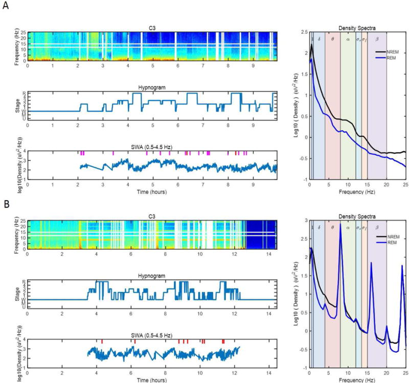
Spectral analysis adjudication panel for a high quality signal and a signal with harmonic contamination. Each panel includes a frequency vs. epoch number spectrogram with color-coded power density (top left), a hypnogram (middle left), a slow-wave activity (SWA) vs. epoch number plot (bottom left) and average spectra for NREM and REM sleep (right). White vertical lines in top left plot indicate beginning and end of wake periods, white horizontal lines highlight spindle frequency band. Tick marks in bottom left plot denote epochs removed due to artifacts (pink = slow frequency artifact, red = high frequency artifact, black = both slow and high frequency artifact). (A) Example of a recording that does not meet any of the a priori adjudication rules for exclusion. The spectra summary figure is typical of data from an older person that is included in the analysis. (B) Example of a recording with harmonic contamination is shown. Harmonic contamination can be found at 8, 16 and 24 Hz in the NREM spectra. Data is identified as having a non-physiological component. Data is removed from further analysis according to the a priori adjudication rules. Note that the long-range harmonic contaminations escaped automated artifact detection but were identified during adjudication.

2.6. Statistical Analysis

2.6.1. Artifact Detection

We compared automated artifact detection with visual artifact detection (i.e. the gold standard) by means of contingency tables listing true positive, true negative, false positive and false negative detections. Since the two analyses were performed using different parameters – automated scoring returned a 1/0 classification of each 30-s epoch as artifactual or not, while visual scoring returned, for each 30-s epoch, the number of artifactual 4-s sub-epochs – there was no unique way to define the gold standard. Thus, we considered the agreement between methods as a function of the number of artifactual sub-epochs (1 to 10) required to designate a 30-s epoch as artifactual. Thus, our gold standard ranged from a more “stringent” definition, where we considered a 30-s epoch as containing artifact even if only one of its 4-s sub-epochs had been scored as artifact, to a more “liberal” definition, where we considered a 30-s epoch as containing artifact only if all 10 4-s sub-epochs had been scored as artifact. We computed the sensitivity, specificity, accuracy and Cohen’s Kappa for each of these 10 definitions.

As a secondary analysis, we restricted the comparison to the sole “large” artifacts, that is, the epochs visually scored as containing artifact where the total EEG power was higher than the 99^th percentile for that night. We compared the two classifications with the same procedure as described above.

2.6.2. Spectra Comparison

We used Spearman correlation analysis to determine the strength of association between EEG spectra computed with the commercial system following visual artifact detection and with the automated pipeline. Wilcoxon rank sum tests were used to compare the average spectral power density in NREM and REM sleep in each relevant EEG band between the two approaches. In addition, we investigated the intra-participant Spearman correlation between the power density values computed for each method across all epochs of sleep, and we plotted the histogram of the r values.

We constructed Bland-Altman plots to examine the agreement between average power densities in NREM and REM computed with the two approaches for the different frequency bands. In these representations, the differences in power density between the two methods are plotted against the means of the two methods.

2.7. Software Tools

We developed and made publicly available the tool box used to conduct the analyses described in this paper, named SpectralTrainFig and available at https://www.sleepdata.org/community/tools/nsrr-spectraltrainfig. SpectralTrainFig contains the pipeline for spectral analysis with prior artifact detection described above, and features a user-friendly graphic user interface for the analysis of multiple recordings with different options. The user is prompted to select the folder where the data resides, the channels to analyze and the reference channels. Additional functionalities are computation of spectral coherence, decontamination from ECG interference³⁹, and sleep cycle-specific analysis⁴⁰. All the code was implemented in Matlab® (The Mathworks, Inc., Natick, MA), version R2015b, and is periodically updated and improved following user feedback. Figure 2 shows the Graphic User Interface of the tool.

Figure 2.

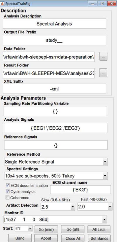
Graphic User Interface of SpectralTrainFig. The user can select data folders, signals to be analyzed, spectral settings, optional ECG decontamination, cycle analysis and coherence computation.

3. Results

3.1. Pipeline Performance and Adjudication

3.1.1. Pipeline Processing Speed

Our open source pipeline was designed to replicate the results of the standard analysis in an automatic way. The generation of average EEG power spectra for NREM and REM sleep including automated artifact detection took approximately 8 seconds per recording on a 3.50 GHz processor, 32 GB RAM system. Approximately 15 additional seconds were required to save adjudication figures to a Microsoft PowerPoint file and numeric results to Excel files. In contrast, the time to perform manual artifact removal and spectral analysis with the commercial system was between 1 and 2 hours per recording.

3.1.2. Visual Verification and Adjudication of Spectral Results

After visual review, nine studies (5%) were excluded from further analysis. The primary reasons for exclusion were the presence of non-physiological signal components and excessive artifacts within the signals during sleep. In the perspective of a big data analysis, which prioritizes computing speed over data retention, we removed these records entirely from the analysis rather than attempt to identify recording segments that could be analyzed, which could also introduce bias. Figure 1 shows examples of visual summaries for representative included and excluded recordings.

3.2. Validation: Artifact Detection

We report the statistics on the global performance of the automated artifact detection method in Table 1. We analyzed 86,250 NREM epochs and 20,717 REM epochs from the sample of 161 participants (excluding 9 participants as described above). Of note, although the method specificity is very high (96.8 to 99.4% in NREM, 96.9 to 99.1% in REM sleep) and consequently the accuracy is high (due to the higher proportion of epochs scored as non-artifact compared to epochs scored as artifact), the sensitivity is low (max sensitivity = 38% to recognize as artifact an epoch of NREM sleep with at least four visually identified sub-epochs with artifacts). The performance of the automated classifier varies as the criterion for defining visual classification changes, that is, with the number x of sub-epochs with artifact needed to define an epoch with artifact. The best agreement, as indicated by Cohen’s kappa, is obtained for x=2 in NREM and x=3 in REM, where x represents the minimum number of artifactual 4-s subepochs needed to define a 30-s epoch as artifactual.

Table 1.

Performance statistics of the automated artifact detector as compared to visual artifact scoring, when considering all visually scored artifacts.

	NREM epochs (N=86,250)							REM epochs (N=20,717)
Th	N art	sens	spec	acc	PPV	NPV	K	N art	sens	spec	acc	PPV	NPV	K
1	8799	26.66	99.36	91.94	82.52	92.26	0.37	6327	9.06	99.08	71.59	81.28	71.25	0.11
2	6904	31.94	99.20	93.81	77.56	94.37	0.43	3997	12.98	98.89	82.31	73.62	82.62	0.17
3	4347	36.62	98.47	95.36	56.00	96.70	0.42	1986	18.78	98.23	90.61	52.91	91.94	0.24
4	2485	38.11	97.74	96.02	33.31	98.16	0.34	1037	22.28	97.59	93.82	32.77	95.97	0.23
5	1293	35.19	97.19	96.26	16.00	99.00	0.20	511	25.05	97.14	95.37	18.16	98.09	0.19
6	653	27.72	96.89	96.37	6.37	99.43	0.09	274	27.37	96.92	96.00	10.64	99.01	0.14
7	400	23.00	96.80	96.45	3.24	99.63	0.05	142	23.94	96.74	96.24	4.82	99.46	0.07
8	283	21.55	96.76	96.52	2.15	99.73	0.03	80	25.00	96.68	96.40	2.84	99.70	0.04
9	226	21.24	96.75	96.55	1.69	99.79	0.03	43	30.23	96.65	96.51	1.84	99.85	0.03
10	194	20.10	96.74	96.57	1.37	99.81	0.02	30	33.33	96.64	96.55	1.42	99.90	0.02

Th: sub-epoch threshold indicating the minimum number of visually identified artifactual 4-s sub-epochs that needed to be present within a 30-s epoch in order to consider this epoch as artifactual. N art: number of 30-s epochs that are considered artifactual with the corresponding sub-epoch threshold. Sens: sensitivity; spec: specificity; acc: accuracy; PPV: positive predictive value; NPV: negative predictive value; K: Cohen’s kappa. The automated pipeline detected 2843 epochs with artifact in NREM and 705 epochs with artifact in REM.

Accuracy and Cohen’s Kappa did not differ between control and cognitively impaired subjects, for any of the 10 criteria, according to the Wilcoxon’s rank sum test (P>0.06).

In Table 2 we report the artifact detection performance when the analysis is restricted to large artifacts only. The sensitivity for these artifacts, that are the most likely to confound the spectral analysis, is very high.

Table 2.

Performance statistics of the automated artifact detector as compared to visual artifact scoring, when considering only the visually scored artifacts having total power greater than the 99% percentile.

	NREM epochs (N=86,250)							REM epochs (N=20,717)
Th	N art	sens	spec	acc	PPV	NPV	K	N art	sens	spec	acc	PPV	NPV	K
1	579	81.35	97.23	97.12	16.57	99.87	0.27	170	75.29	97.19	97.01	18.16	99.79	0.28
2	560	82.14	97.22	97.12	16.18	99.88	0.26	159	78.62	97.18	97.04	17.73	99.83	0.28
3	443	84.88	97.12	97.06	13.23	99.92	0.22	122	82.79	97.07	96.98	14.33	99.90	0.24
4	306	86.60	97.00	96.96	9.32	99.95	0.16	90	85.56	96.96	96.91	10.92	99.94	0.19
5	163	87.73	96.86	96.85	5.03	99.98	0.09	51	88.24	96.81	96.79	6.38	99.97	0.11
6	66	86.36	96.77	96.76	2.00	99.99	0.04	28	85.71	96.71	96.69	3.40	99.98	0.06
7	41	80.49	96.74	96.73	1.16	99.99	0.02	11	90.91	96.64	96.64	1.42	100.00	0.03
8	28	71.43	96.73	96.72	0.70	99.99	0.01	8	87.50	96.63	96.63	0.99	100.00	0.02
9	20	70.00	96.72	96.71	0.49	99.99	0.01	6	83.33	96.62	96.62	0.71	100.00	0.01
10	18	72.22	96.72	96.71	0.46	99.99	0.01	5	80.00	96.62	96.61	0.57	100.00	0.01

Th: sub-epoch threshold indicating the minimum number of visually identified artifactual 4-s sub-epochs that needed to be present within a 30-s epoch in order to consider this epoch as artifactual. N art: number of 30-s epochs that are considered artifactual with the corresponding sub-epoch threshold. Sens: sensitivity; spec: specificity; acc: accuracy; PPV: positive predictive value; NPV: negative predictive value; K: Cohen’s kappa. The automated pipeline detected 2843 epochs with artifact in NREM and 705 epochs with artifact in REM.

Figure 3 illustrates the performance of the two artifact detection methods exemplified for a short segment of raw EEG data. In general, the automated detector is very accurate at detecting large, obvious artifacts that affect the slow band or the fast band descriptor. In the example, the two larger artifacts at 50 and 240 s, approximately, are detected by the automatic algorithm, while the smaller one at 80 s is missed.

Figure 3.

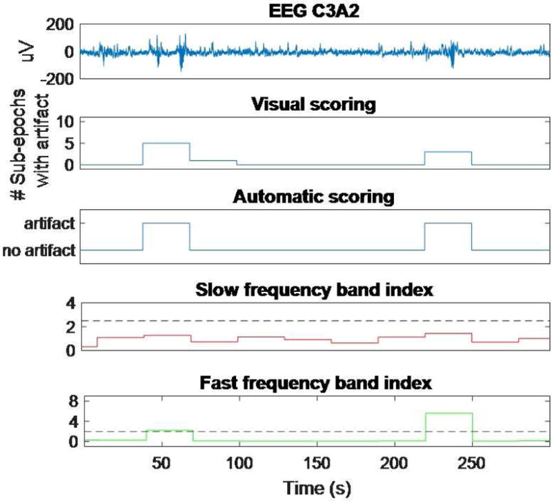
Comparison between visual and automated artifact scoring exemplified for a 5-min segment of sleep EEG. The top panel shows the raw EEG signal. The second panel shows, for each 30-s epoch, the number of 4-s sub-epochs with artifacts according to the visual scoring. The third panel shows the automatic artifact scoring for each 30-s epoch. The two bottom panels show the two indices used to derive the automated scoring, each with its respective threshold (dashed lines). For details, see Methods.

The visual artifact detection procedure resulted in the removal of 3.55% and 8.51% of recording time spent in NREM sleep and REM sleep, respectively. The automatic artifact detection procedure resulted in the removal of 3.30% and 3.40% of recording time spent in NREM sleep and REM sleep, respectively.

3.3. Validation: Spectra characteristics

We computed sleep EEG spectra characteristics for the analysis dataset with both the standard approach and the automated pipeline.

Spearman correlations between mean log-transformed spectral power density obtained with the standard and the automated procedures ranged between 0.99 and 1.00 for all frequency bands (Table 3) for both REM and NREM sleep. Bland-Altman plots showed good agreement between spectral analyses results computed with the two procedures (Figure 4). For all bands, the Wilcoxon test showed no significant difference between the means of the two distributions. Mean differences in spectral power obtained with the two approaches ranged between 0.46% (for NREM delta power) and 10.10% (for NREM beta power). Differences in spectral power, both absolute and relative, did not differ between healthy and cognitively impaired subjects (p> 0.2).

Table 3.

Spectral power density in characteristic EEG frequency bands computed with the standard approach and the automated pipeline.

	Band limits (Hz)	Power density (Standard) (log10(uV2/Hz)) mean (std)	Power density (Automated) (log10(uV2/Hz)) mean (std)	Absolute Difference (log10(uV2/Hz)) mean (std)	%-Difference mean (std)	Spearman r
NREM
Slow Osc.	0.25–1	2.34 (0.18)	2.36 (0.19)	0.02 (0.02)	0.65 (0.63)	0.99
Delta	1.25–4	1.35 (0.17)	1.35 (0.17)	0.01 (0.01)	0.46 (0.65)	1.00
Theta	4.25–8	0.87 (0.21)	0.87 (0.21)	0.00 (0.01)	0.47 (0.71)	1.00
Alpha	8.25–12	0.55 (0.22)	0.56 (0.22)	0.01 (0.01)	1.74 (3.41)	1.00
Sigma	12.25–15	0.16 (0.21)	0.17 (0.21)	0.01 (0.01)	6.73 (12.16)	1.00
Beta	15.25–20	−0.27 (0.19)	−0.26 (0.19)	0.01 (0.02)	10.10 (25.04)	1.00
REM
Slow Osc.	0.25–1	1.99 (0.23)	2.03 (0.25)	0.04 (0.05)	1.85 (1.69)	0.99
Delta	1.25–4	0.95 (0.17)	0.96 (0.17)	0.02 (0.04)	2.09 (3.10)	0.99
Theta	4.25–8	0.61 (0.22)	0.62 (0.22)	0.01 (0.02)	2.03 (5.83)	0.99
Alpha	8.25–12	0.41 (0.26)	0.41 (0.26)	0.01 (0.01)	4.12 (12.44)	1.00
Sigma	12.25–15	0.07 (0.25)	0.07 (0.26)	0.01 (0.01)	7.97 (18.24)	1.00
Beta	15.25–20	−0.19 (0.24)	−0.19 (0.24)	0.01 (0.01)	7.58 (18.25)	1.00

Differences between average spectral power density values computed with the two approaches in REM and NREM are all not significant (p > 0.05). All correlations are statistically significant (p <0.01). In the standard approach, spectra were calculated for consecutive 30-s epochs after removing 4-s sub-epochs with visually identified artifacts and then averaging the remaining artifact free 4-s spectra from up to ten overlapping 4-s sub-epochs. In the automated approach, epochs with automatically scored artifact were excluded from the analysis. It must be noted that activity in the slow oscillation band (0.25–1 Hz) is often due to sweating artifact.

Figure 4.

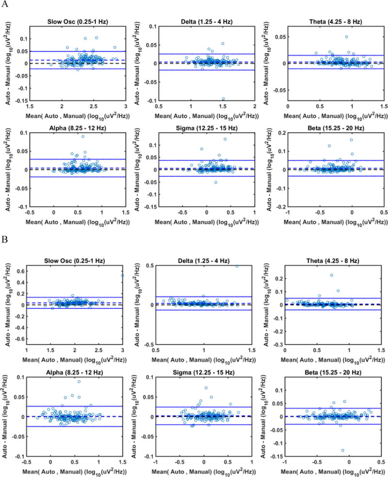
Bland-Altman plots of power density computed with standard and automated pipeline for various frequency bands. Bland-Altman plots are provided to show the agreement between the two approaches. Differences in power density between the two approaches (y-axis) are plotted against the means of them (x-axis). Each blue circle represents results for a single participant. The dashed blue horizontal line corresponds to the average difference between the two approaches. The two dotted blue lines correspond to plus/minus 2 standard deviations of the difference. Data are shown for NREM sleep (A) and REM sleep (B) separately.

Figure 5 shows the distribution of per-individual Spearman correlation for epoch-by-epoch log-transformed spectral power in each band between the two methods. For the large majority of participants, very high correlation coefficients were obtained. Participants for whom the correlation was lower, were in general those with larger numbers of visually identified artifacts, as shown in supplemental Figure S1.

Figure 5.

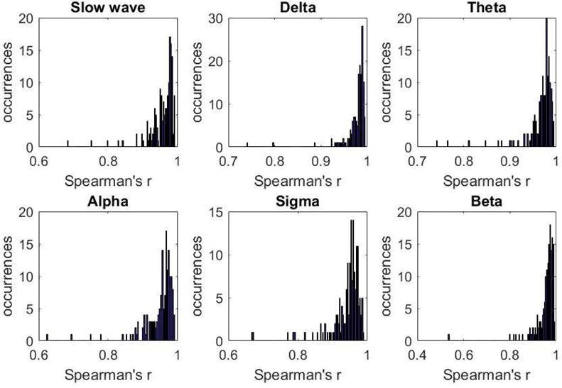
Histograms of Spearman’s correlation coefficients between power densities computed following standard and automated artifact removal. Individual correlation coefficients are from 161 participants and were calculated across 30-s epochs of sleep that remained after artifact removal.

To investigate the effect of automated artifact rejection on spectral power, we also plotted power in the relevant bands obtained with the traditional approach, with the automated approach with no artifact rejection, and with automated approach with artifact rejection. An example is shown in Figure S2.

As a final analysis, we computed mean spectral power density in each band, for consecutive NREM-REM sleep cycles. We defined sleep cycles as periods of NREM sleep lasting at least 15 minutes, and terminated by either 1) the end of a period of stage REM sleep of any duration for cycle 1 or at least 5 minutes for other cycles, or 2) a period of wake or stage N1 for at least 15 contiguous minutes. This analysis by cycles revealed that the correlation coefficients between the standard and the automated approach ranged between 0.98 and 1 while no significant differences in power density were found (Wilcoxon). Figure S3 shows the results.

4. Discussion

We implemented an open-source, user-friendly tool for both automating artifact rejection and for computing EEG spectral analysis. This automated pipeline reduces analysis time 100-fold with respect to standard analysis, which requires visual artifact scoring by a sleep expert. Although overall epoch-by-epoch sensitivity for detecting artifacts was low to modest, major artifacts, that are most likely to distort average spectral estimates, were detected with high sensitivity. The automated pipeline produced average power densities and power densities across the night that were nearly identical to values computed with traditional visual editing. In particular, correlations between EEG spectral power density computed with the two methods were greater than 0.99 for both NREM and REM, and differences between power densities in the relevant EEG bands ranged between 0.5 and 10% on average.

Research opportunities to aggregate and analyze large amounts of data are gaining increasing attention. Publicly available programs, source code, and documentation reduce the startup time for new users, facilitate the ability to replicate analyses, and provide a platform for technology-enabled research. Additional details and cohort specific spectral analysis information are made available from the National Sleep Research Resource (NSRR)⁴¹ website (http://sleepdata.org). To optimize the uptake of the tools, a detailed standard operating procedure for adjudication was developed.

A focus of our work was detection and elimination of artifact in the EEG channel, which could be due to cardiac, electrode, environmental, muscle and ocular artifact is a known limitation of quantitative analysis⁴². While traditional approaches have used manual artifact removal¹⁷, we adapted an automated threshold-based artifact detection approach described in the literature³⁸ supported by a report demonstrating that physiology-driven, threshold-based artifact detection can perform well in comparison to more sophisticated methods⁴³. We combined this automated method with a procedure involving quick expert review (adjudication). We found that visual adjudication of a one-page summary per recording identified studies with substantial missing data, electrical (60 Hz) contamination, environmental contamination and cardiac contamination that escaped threshold-based artifact detection. Taken together, the current analyses support the utility of using a single artifact detection approach that removes epochs with large non-physiological components in the 0.5–4.5 Hz and 20–40 Hz range combined with a brief review of informative summary figures to identify problematic recordings as an acceptable a and efficient approach for generating spectral analysis output for large numbers of studies.

The artifacts that are not picked up by the algorithms seem to occur at frequencies that are often not in the range of spectra commonly examined for clinical purposes and for many sleep research purposes, and did not materially affect the summary spectra results. Nonetheless, while the artifact rejection method is suitable for spectral analysis of the EEG on a macroscopic scale, it is important to recognize that there are qEEG analyses for which more sensitive, and perhaps multiple, artifact detection methods are needed, such as for studies of transient EEG events In our analysis of sleep spindles⁴⁴, we additionally incorporated statistical filtering on per-epoch Hjorth parameters, RMS and clipped signals to increase detection sensitivity.

The amount of recording time that was rejected with the visual and automated methods was similar for NREM sleep (3.6% for the visual scoring, 3.3% for the automated scoring), while for REM sleep the automated method removed a smaller proportion (3.4%) with respect to the visual method (8.5%). This difference is most likely due the presence of artifacts caused by interspersed rapid-eye movements, REM sleep twitches or transitions into and out of REM accompanied by some brief movement, which escaped automated detection. The process for rejecting epochs also was influenced by the size of the epochs, since individual short artifacts of 4 s could be rejected in the visual method, while in the automated pipeline the artifact needed to be pervasive over the 30-s epoch. This difference also influenced the performance assessment, as the gold standard could not be uniquely defined. The best performance was obtained with the presence of a minimum of two 4-s artifacts (x=2) within a 30-s epoch of NREM sleep and three 4-s artifacts (x=3) within a 30-s epoch of REM sleep. For smaller values of x, the sensitivity decreases, as shorter artifacts scored visually may be harder to detect by the automated detector, and it is particularly low in REM. In NREM, the sensitivity decreases also for increasing threshold values.

We considered application of additional and customized artifact detection algorithms. EEG artifact detection utilities are available that include functions for identifying a range of environmentally and physiologically generated artifacts^25,27,45. Open source tools such as Brainstorm⁴⁶ and EEGlab⁴⁷ include a large set of artifact detection methods that support spectral analysis of EEG data and interactive/automated artifact detection. Although the analysis procedures are sophisticated, Brainstorm and EEGlab were developed to primarily analyze EEG evoked response data, and the artifact detection methods are based on Independent Component Analysis, which requires multiple leads and is computationally more intensive. The pipeline presented in our study is designed for sleep analysis, providing measures that are tailored to represent sleep rhythms, available for analysis in customized spreadsheets. Artifact rejection utilizes a simple approach that does not require multiple leads, and includes sleep-dedicated features, such as ECG decontamination and cycle-specific analysis. In addition, our pipeline offers a user-friendly approach when working with large datasets of hundreds of recordings at a time.

There are many commercial products that include spectral analysis of sleep studies and provide artifact detection such as Prana Software (Strasbourg, France)⁴⁸. However, commercial sleep analysis software that includes spectral analysis and automatic artifact detection is often costly, and code is proprietary. Moreover, application of additional and customized artifact detection algorithms that identify physiological and environmental artifacts seemed cumbersome and potentially subjective.

Future automation of visual adjudication rules may be possible, resulting in a completely automated pipeline. In addition, the spectral analysis performed in the pipeline currently relies on manually staged sleep, but could be integrated into an automated sleep staging approach in the future. Artifact detection could be used to eliminate noisy epochs prior to feature extraction for sleep stage classification or provide an additional feature for wakefulness detection. As some artifacts, such as in the case of Figure 1B, are only present for part of the night, future iterations of the program might allow for selection of non-artifactual portions of the recordings, in order to retain a larger amount of data.

One limitation of the study is that the algorithms were tested using data from a single, elderly cohort of women. Additional validation studies in different populations and with different spectral parameters/methods are required to better understand how the current analysis pipeline performs compared to standard manual artifact detection. Given the challenges in EEG collection in older individuals and data collected in in-home settings, however, our estimates of agreement are likely conservative compared to data obtained in young individuals or in controlled laboratory settings. While we focused our analysis on absolute power in each band, there is also interest in calculating relative power, i.e., absolute power in a certain band divided by total power (up to a certain frequency). Since the pipeline produces the epoch-by-epoch spectral power density values for each frequency bin, the relative power can easily be derived, and we tested it in our cohort. There was good agreement between the two approaches in this case as well, with all p values from the Wilcoxon t tests showing no significant differences between spectral power in each band computed with the two approaches and percentage differences ranging from 0.7 to 4.8%.

Our pipeline was designed with the NSRR datasets in mind, accommodating input data that are in European Data Format (EDF) for signals and XML for annotations. However, our approach is easily generalizable to any sleep recording, as most sleep acquisition systems can output data in EDF. The tool has been developed in Matlab, which is a commercial software. Future implementation in versions compatible with GNU-Octave, could provide a free alternative.

5. Conclusion

In summary, the study results demonstrate that automated artifact detection can be applied in conjunction with spectral analysis efficiently and maintain good agreement with gold standard methods. The analysis pipeline resulted in a decrease of two orders of magnitude in the amount of time required to perform spectral analysis. This computational advance has enabled spectral analyses of thousands of recordings that aggregate across several NIH funded cohorts (data posted at sleepdata.org) and has the potential to provide new insights into individual and subgroup differences in sleep, cognitive development, and cognitive decline. In this perspective, we predict that the statistical power that is realized by processing large numbers of recordings will likely outweigh the effects of residual differences in artifact detection between hand-scored and automatically scored recordings for many purposes. Employing an open source analysis framework is consistent with national data, analysis and computational initiatives⁵² that encourage availability of source code so that the research community can replicate published analyses^49,50. Our methods will address an important gap on the path to next-generation national sleep research opportunities⁵¹.

The publicly released software provides the scientific community with a suite of tools designed to support large-scale spectral analyses of sleep studies. Future work will involve expanding the pipeline to include additional artifact detection approaches, analyses of transient events, and multivariate approaches. Incorporating higher order statistics, EMG driven EEG artifact detection, and sleep/wake-state aware artifact detection could greatly enhance the applicability of the analysis pipeline to other research problems. Extending the pipeline to include additional methods for analyzing unique features of the EEG (e.g., spindles) or cross-signal analysis could accelerate the development of an array of physiological metrics for use in a wide range of genomic, precision medicine and other research. Future enhancements may include computational informatics that combine analyses with distributing computing and reporting functionality. Such computational informatics derived from methods used in computer science to address Big Data analysis are encouraged by Big Data to Knowledge initiatives, but have only been applied sparingly in sleep analyses^52,53.

Supplementary Material

2

Figure S1: Relationship between the number of artifacts identified by the standard approach and the agreement in power density between standard and automated approach. The scatter plot shows, for each participant, the number of 4-s epochs identified as artifact on the x axis, and the mean Spearman correlation coefficient for the six bands between the two approaches. It can be noticed that, as expected, recording with a higher number of artifacts have lower correlation between methods.

Figure S2: Spectral power density in the slow oscillation bands obtained with the traditional method (top panel), the automated pipeline with no artifact rejection (middle panel) and the automated pipeline with artifact rejection (bottom panel). The automated artifact rejection method identifies major artifacts that affect spectral density estimation.

Figure S3: Power densities per sleep cycle for (a) NREM sleep and (b) REM sleep. The bars represented mean values (± SEM)) for each band. Grey bars represent results of the standard approach while black bars show results of the automated approach.

Highlights.

• An automated pipeline for spectral analysis of the sleep electroencephalogram is proposed, which includes automated artifact detection

• Our pipeline is featured in the framework of the National Sleep Research Resource, for efficient analysis of large cohorts of polysomnographic data

• We validate our method by comparing it with a standard approach which employs manual artifact scoring and the use of a commercial software

References

- 1.AESCHBACH D, BORBÉLY AA. All-night dynamics of the human sleep EEG. J Sleep Res. 1993;2:70–81. doi: 10.1111/j.1365-2869.1993.tb00065.x. [DOI] [PubMed] [Google Scholar]
- 2.Achermann P, Dijk D, Brunner DP, Borbély AA. A model of human sleep homeostasis based on EEG slow-wave activity: quantitative comparison of data and simulations. Brain Res Bull. 1993;31:97–113. doi: 10.1016/0361-9230(93)90016-5. [DOI] [PubMed] [Google Scholar]
- 3.Petit D, Gagnon J, Fantini ML, Ferini-Strambi L, Montplaisir J. Sleep and quantitative EEG in neurodegenerative disorders. J Psychosom Res. 2004;56:487–96. doi: 10.1016/j.jpsychores.2004.02.001. [DOI] [PubMed] [Google Scholar]
- 4.Walker MP, Stickgold R. Sleep-dependent learning and memory consolidation. Neuron. 2004;44:121–33. doi: 10.1016/j.neuron.2004.08.031. [DOI] [PubMed] [Google Scholar]
- 5.Carskadon MA, Dement WC. Normal human sleep: an overview. Principles and practice of sleep medicine. 2005;4:13–23. [Google Scholar]
- 6.Coburn KL, Lauterbach EC, Boutros NN, Black KJ, Arciniegas DB, Coffey CE. The value of quantitative electroencephalography in clinical psychiatry: a report by the Committee on Research of the American Neuropsychiatric Association. J Neuropsychiatry Clin Neurosci. 2006;18:460–500. doi: 10.1176/jnp.2006.18.4.460. [DOI] [PubMed] [Google Scholar]
- 7.Moretti D, Zanetti O, Binetti G, Frisoni G. Quantitative EEG markers in mild cognitive impairment: degenerative versus vascular brain impairment. International Journal of Alzheimer’s Disease. 2012;2012 doi: 10.1155/2012/917537. [DOI] [PMC free article] [PubMed] [Google Scholar]
- 8.Borbély AA. A two process model of sleep regulation. Hum Neurobiol. 1982 [PubMed] [Google Scholar]
- 9.Achermann P, Borbely A. Low-frequency (< 1 Hz) oscillations in the human sleep electroencephalogram. Neuroscience. 1997;81:213. doi: 10.1016/s0306-4522(97)00186-3. [DOI] [PubMed] [Google Scholar]
- 10.Ferrarelli F, Huber R, Peterson MJ, et al. Reduced sleep spindle activity in schizophrenia patients. Am J Psychiatry. 2007 doi: 10.1176/ajp.2007.164.3.483. [DOI] [PubMed] [Google Scholar]
- 11.Anghinah R, Kanda PAM, Lopes HF, et al. Alzheimer’s disease qEEG: spectral analysis versus coherence. which is the best measurement? Arq Neuropsiquiatr. 2011;69:871–4. doi: 10.1590/s0004-282x2011000700004. [DOI] [PubMed] [Google Scholar]
- 12.Geiger A, Huber R, Kurth S, Ringli M, Jenni OG, Achermann P. The sleep EEG as a marker of intellectual ability in school age children. Sleep. 2011;34:181–9. doi: 10.1093/sleep/34.2.181. [DOI] [PMC free article] [PubMed] [Google Scholar]
- 13.Kurth S, Achermann P, Rusterholz T, LeBourgeois MK. Development of brain EEG connectivity across early childhood: does sleep play a role? Brain sciences. 2013;3:1445–60. doi: 10.3390/brainsci3041445. [DOI] [PMC free article] [PubMed] [Google Scholar]
- 14.Huber R, Ghilardi MF, Massimini M, Tononi G. Local sleep and learning. Nature. 2004;430:78–81. doi: 10.1038/nature02663. [DOI] [PubMed] [Google Scholar]
- 15.Aeschbach D, Cutler AJ, Ronda JM. A role for non-rapid-eye-movement sleep homeostasis in perceptual learning. J Neurosci. 2008;28:2766–72. doi: 10.1523/JNEUROSCI.5548-07.2008. [DOI] [PMC free article] [PubMed] [Google Scholar]
- 16.Aeschbach D, Dijk D, Trachsel L, Brunner DP, Borbély AA. Dynamics of slow-wave activity and spindle frequency activity in the human sleep EEG: effect of midazolam and zopiclone. 1994 doi: 10.1038/sj.npp.1380110. [DOI] [PubMed] [Google Scholar]
- 17.Aeschbach D, Lockyer B, Dijk D, et al. Use of transdermal melatonin delivery to improve sleep maintenance during daytime. Clinical Pharmacology & Therapeutics. 2009;86:378–82. doi: 10.1038/clpt.2009.109. [DOI] [PMC free article] [PubMed] [Google Scholar]
- 18.Arbon EL, Knurowska M, Dijk DJ. Randomised clinical trial of the effects of prolonged-release melatonin, temazepam and zolpidem on slow-wave activity during sleep in healthy people. J Psychopharmacol. 2015;29:764–76. doi: 10.1177/0269881115581963. [DOI] [PubMed] [Google Scholar]
- 19.Landolt H, Dijk D. Genetic basis of sleep in healthy humans Principles and practice of sleep medicine. 5th. St Louis (MO): Elsevier Saunders; 2011. pp. 175–83. [Google Scholar]
- 20.Dietsch G. Fourier Analysis von Electroencephalogrammen des Menschen. Pflüger’s Arch Ges Physiol. 1932;220:106–12. [Google Scholar]
- 21.Priestley MB. Spectral analysis and time series. 1981 [Google Scholar]
- 22.Achermann P. EEG analysis applied to sleep. Epileptologie. 2009;26:28–33. [Google Scholar]
- 23.Jaffe DA. Spectrum analysis tutorial, Part 2: Properties and applications of the discrete Fourier transform. Computer Music Journal. 1987;11:17–35. [Google Scholar]
- 24.Delorme A, Sejnowski T, Makeig S. Enhanced detection of artifacts in EEG data using higher-order statistics and independent component analysis. Neuroimage. 2007;34:1443–9. doi: 10.1016/j.neuroimage.2006.11.004. [DOI] [PMC free article] [PubMed] [Google Scholar]
- 25.Anderer P, Roberts S, Schlogl A, et al. Artifact processing in computerized analysis of sleep EEG - a review. Neuropsychobiology. 1999;40:150–7. doi: 10.1159/000026613. [DOI] [PubMed] [Google Scholar]
- 26.James CJ, Hesse CW. Independent component analysis for biomedical signals. Physiol Meas. 2004;26:R15. doi: 10.1088/0967-3334/26/1/r02. [DOI] [PubMed] [Google Scholar]
- 27.Nolan H, Whelan R, Reilly R. FASTER: fully automated statistical thresholding for EEG artifact rejection. J Neurosci Methods. 2010;192:152–62. doi: 10.1016/j.jneumeth.2010.07.015. [DOI] [PubMed] [Google Scholar]
- 28.Gao J, Yang Y, Sun J, Yu G. Automatic removal of various artifacts from EEG signals using combined methods. J Clin Neurophysiol. 2010;27:312–20. doi: 10.1097/WNP.0b013e3181f534f4. [DOI] [PubMed] [Google Scholar]
- 29.Djonlagic I, Aeschbach D, Litwack Harrison S, et al. Associations between Quantitative Sleep EEG Data and Subsequent Cognitive Decline in Community-Dwelling Older Women. Journal of Sleep and Sleep Disorders Research. 2014:A339. doi: 10.1111/jsr.12666. [DOI] [PMC free article] [PubMed] [Google Scholar]
- 30.Cummings SR, Nevitt MC, Browner WS, et al. Risk factors for hip fracture in white women. N Engl J Med. 1995;332:767–74. doi: 10.1056/NEJM199503233321202. [DOI] [PubMed] [Google Scholar]
- 31.Blackwell T, Yaffe K, Ancoli-Israel S, et al. Poor sleep is associated with impaired cognitive function in older women: the study of osteoporotic fractures. The Journals of Gerontology Series A: Biological Sciences and Medical Sciences. 2006;61:405–10. doi: 10.1093/gerona/61.4.405. [DOI] [PubMed] [Google Scholar]
- 32.Redline S, Sanders MH, Lind BK, et al. Methods for obtaining and analyzing unattended polysomnography data for a multicenter study. Sleep. 1998;21:759–68. [PubMed] [Google Scholar]
- 33.Iber C, Ancoli-Israel S, Chesson A, Quan SF. The AASM manual for the scoring of sleep and associated events: rules, terminology, and technical specifications. 1st. Westchester, IL: 2007. [Google Scholar]
- 34.Cooley JW, Tukey JW. An algorithm for the machine calculation of complex Fourier series. Mathematics of computation. 1965;19:297–301. [Google Scholar]
- 35.Welch PD. The use of fast Fourier transform for the estimation of power spectra: A method based on time averaging over short, modified periodograms. IEEE Transactions on audio and electroacoustics. 1967;15:70–3. [Google Scholar]
- 36.Bloomfield P. Fourier analysis of time series: an introduction. John Wiley & Sons; 2004. [Google Scholar]
- 37.Harris FJ. On the use of windows for harmonic analysis with the discrete Fourier transform. Proc IEEE. 1978;66:51–83. [Google Scholar]
- 38.Buckelmüller J, Landolt H, Stassen H, Achermann P. Trait-like individual differences in the human sleep electroencephalogram. Neuroscience. 2006;138:351–6. doi: 10.1016/j.neuroscience.2005.11.005. [DOI] [PubMed] [Google Scholar]
- 39.Nakamura M, Shibasaki H. Elimination of EKG artifacts from EEG records: a new method of non-cephalic referential EEG recording. Electroencephalogr Clin Neurophysiol. 1987;66:89–92. doi: 10.1016/0013-4694(87)90143-x. [DOI] [PubMed] [Google Scholar]
- 40.Feinberg I, Floyd T. Systematic trends across the night in human sleep cycles. Psychophysiology. 1979;16:283–91. doi: 10.1111/j.1469-8986.1979.tb02991.x. [DOI] [PubMed] [Google Scholar]
- 41.Dean DA, Goldberger AL, Mueller R, et al. Scaling Up Scientific Discovery in Sleep Medicine: The National Sleep Research Resource. Sleep. 2016 doi: 10.5665/sleep.5774. [DOI] [PMC free article] [PubMed] [Google Scholar]
- 42.Stern JM. Atlas of EEG patterns. Lippincott Williams & Wilkins; 2005. [Google Scholar]
- 43.Delorme A, Sejnowski T, Makeig S. Enhanced detection of artifacts in EEG data using higher-order statistics and independent component analysis. Neuroimage. 2007;34:1443–9. doi: 10.1016/j.neuroimage.2006.11.004. [DOI] [PMC free article] [PubMed] [Google Scholar]
- 44.Purcell S, Manoach D, Demanuele C, et al. Characterizing sleep spindles in 11,630 individuals from the National Sleep Research Resource. Nature Communications. 2017;8 doi: 10.1038/ncomms15930. ncomms 15930. [DOI] [PMC free article] [PubMed] [Google Scholar]
- 45.Lawhern V, Hairston WD, Robbins K. DETECT: A MATLAB toolbox for event detection and identification in time series, with applications to artifact detection in EEG signals. PloS one. 2013;8:e62944. doi: 10.1371/journal.pone.0062944. [DOI] [PMC free article] [PubMed] [Google Scholar]
- 46.Tadel F, Baillet S, Mosher JC, Pantazis D, Leahy RM. Brainstorm: a user-friendly application for MEG/EEG analysis. Computational intelligence and neuroscience. 2011;2011:8. doi: 10.1155/2011/879716. [DOI] [PMC free article] [PubMed] [Google Scholar]
- 47.Delorme A, Makeig S. EEGLAB: an open source toolbox for analysis of single-trial EEG dynamics including independent component analysis. J Neurosci Methods. 2004;134:9–21. doi: 10.1016/j.jneumeth.2003.10.009. [DOI] [PubMed] [Google Scholar]
- 48.Zoubek L, Charbonnier S, Lesecq S, Buguet A, Chapotot F. A two-steps sleep/wake stages classifier taking into account artefacts in the polysomnographic signals. IFAC Proceedings Volumes. 2008;41:5227–32. [Google Scholar]
- 49.LeVeque RJ, Mitchell IM, Stodden V. Reproducible research for scientific computing: Tools and strategies for changing the culture. Computing in Science and Engineering. 2012;14:13. [Google Scholar]
- 50.Margolis R, Derr L, Dunn M, et al. The National Institutes of Health’s Big Data to Knowledge (BD2K) initiative: capitalizing on biomedical big data. J Am Med Inform Assoc. 2014;21:957–8. doi: 10.1136/amiajnl-2014-002974. [DOI] [PMC free article] [PubMed] [Google Scholar]
- 51.Zee PC, Badr MS, Kushida C, et al. Strategic opportunities in sleep and circadian research: report of the Joint Task Force of the Sleep Research Society and American Academy of Sleep Medicine. Sleep. 2014;37:219–27. doi: 10.5665/sleep.3384. [DOI] [PMC free article] [PubMed] [Google Scholar]
- 52.Dean DA, Forger DB, Klerman EB. Taking the lag out of jet lag through model-based schedule design. PLoS Comput Biol. 2009;5:e1000418. doi: 10.1371/journal.pcbi.1000418. [DOI] [PMC free article] [PubMed] [Google Scholar]
- 53.Dean IIDA, Adler GK, Nguyen DP, Klerman EB. Biological Time Series Analysis Using a Context Free Language: Applicability to Pulsatile Hormone Data. PloS one. 2014;9:e104087. doi: 10.1371/journal.pone.0104087. [DOI] [PMC free article] [PubMed] [Google Scholar]
Associated Data
This section collects any data citations, data availability statements, or supplementary materials included in this article.
Supplementary Materials