Identification of Clinically Meaningful Plasma Transfusion Subgroups Using Unsupervised Random Forest Clustering

Abstract

Statistical techniques such as propensity score matching and instrumental variable are commonly employed to “simulate” randomization and adjust for measured confounders in comparative effectiveness research. Despite such adjustments, the results of these methods apply essentially to an “average” patient. However, as patients show significant heterogeneity in their responses to treatments, this average effect is of limited value. It does not account for individual level variabilities, which can deviate substantially from the population average. To address this critical problem, we present a framework that allows the discovery of clinically meaningful homogeneous subgroups with differential effects of plasma transfusion using unsupervised random forest clustering. Subgroup analysis using two blood transfusion datasets show that considerable variablilities exist between the subgroups and population in both the treatment effect of plasma transfusion on bleeding and mortality and risk factors for these outcomes. These results support the customization of blood transfusion therapy for the individual patient.

Introduction

Numerous studies and published guidelines encourage the appropriate use of fresh frozen plasma (FFP) and recommend specific circumstances for FFP transfusions. Although there is some variation about the definition of appropriate FFP transfusion, most guidelines suggest a cutoff in the international normalized ratio (INR) of 1.5 (i.e. Prothrombin time > 1.5 × normal).¹ However, the documented compliance to these guidelines is poor.^2–4 Data suggest that inappropriate FFP transfusion varies from institution to institution and ranges from about 10% to 83%.^2;5 Moreover, FFP transfusion puts the patient at risk of a variety of outcomes. FFP transfusion is associated with high risk of transfusion-associated circulatory overload (TACO),⁶ transfusion-associated lung injury (TRALI),⁷ perioperative bleeding,^8–10 multi-organ failure,⁷ infectious complications, and increase in health resource utilization. Therefore, strategies that can safely reduce the need for FFP transfusion bear high potential for improving patient outcomes. Recognizing that inappropriate plasma transfusions should be avoided, the literature is however not clear about the remaining percentage for which it might be beneficial. Currently, no study or best-practice guidelines exist regarding either patient subpopulation or specific characteristics of those patients who might benefit from FFP transfusion. Identifying the subgroup(s) with the most beneficial; wasteful; harmful, or futile prospect of FFP transfusion can provide an efficient means to improve patient outcomes, reduce unnecessary exposure to treatment adverse effects, and save resources.

Subgroup analysis is an important task in comparative effectiveness research where assessing the effect of a treatment on an outcome is of critical interest. Large observational health care databases provide potentially rich sources of information for data mining and machine learning methods to help research on heterogeneity in patient response to treatments and to guide care-givers’ decisions. Because of the large sample sizes, heterogeneous patient population, and real-world settings, they are suitable for studying either patient-specific or group-specific characteristics with respect to a clinical measure. However, comparative effectiveness research based on observational data is challenged by both selection bias and potential for unmeasured confounding. In usual care settings, many patient and physician factors influence whether a patient is selected for a treatment or not, thus any comparison between treatment groups is subject to bias. Through classical statistical methods such as propensity score matching and instrumental variables, it is possible to adjust for measured confounding and obtain unbiased estimates of treatment effects. These methods however suffer from several known weaknesses described below.

Traditionally, treatment effect is commonly estimated by a regression model where the outcome is regressed against patient covariates and the treatment. The effect is then read off as the corresponding regression coefficient of the treatment variable. However, as patients can show significant heterogeneity in response to a treatment, this “average” effect is not appropriate for describing individual level differential effects. Average superiority of one treatment over another does not necessarily mean the treatment will remain superior for each patient. As a result of heterogeneity in patient characteristics such as genetics, phenotypic, pharmacokinetic, environmental, and socio-economic factors, clinical outcomes for some patients may deviate considerably from the population average. The important relationship between treatment effect and patient heterogeneity has been welled investigated;^11;12 however, comparative effectiveness researchers still rely on inefficient and non-robust classical regression and propensity score methods for estimation of treatment effects in observational studies.

In this study, we provide a three stage framework that allows the discovery of stable, robust and clinically meaningful homogeneous subgroups with differential effects of plasma transfusion on important patient outcomes. In the first step, our proposed framework makes use of the unsupervised random forest (URF) algorithm¹³ to derive a “proximity” or dissimilarity matrix between data points in a mixed-type (continuous and categorical) high dimensional covariate space. In the second step, we use the dissimilarity matrix in a hierarchical clustering algorithm to identify highly similar patient subgroups. Compared to classical parametrically derived propensity scores, the URF subgroup membership represents a more robust covariate balancing score.¹⁴ Thus, treatment effect estimates within subgroups of well-matched clinically homogeneous patients are then conditionally unbiased.¹⁵ In the final step, we applied the doubly robust targeted maximum likelihood estimation (TMLE)^16;17 method to estimate the effect of FFP transfusion on bleeding and mortality in each subgroup. The TMLE further insures against any potential confounding that may still exist in the subgroups.

The framework was applied to two datasets from a single academic institutional blood transfusion datamart¹⁸ to discover subgroups of patients with differential responses to pre-operative or pre-procedural plasma transfusion (PPT) on two important patient outcomes: intra-operative or intra-procedural bleeding and mortality. Using only pre-operative or pre-procedural patient information, a cluster validation technique based on the predictive strength of cluster memberships and treatment assignment indicated that the first dataset consisting of patients undergoing non-cardiac surgery (NCS) can be clustered into six homogeneous subgroups while the second dataset consisting of patients undergoing interventional radiology (IR) procedures can be clustered into five subgroups. With respect to clustering the NCS data set, we found two clusters with harmful effect, two clusters with beneficial effect, and a cluster with no effect of PPT on bleeding. Three clusters showed no effect of PPT on mortality and two clusters showed harmful effects. Similar results were obtained for the IR data set. Compared to previous studies that have shown the population wide harmful effects of plasma transfusion,^3;8–10 the findings in this study suggest the need to consider individualized and/or subgroup effects of plasma transfusion.

To further characterize phenotypes of patients within these subgroups, we applied a random forest feature contribution technique¹⁹ to determine which patient characteristics most strongly predict bleeding or mortality at both the population and individual levels. The feature contributions showed that considerable variabilities exist between population level risk factors and individualize/subgroup level risk factors.

Method

Study Population

This is a retrospective observational cohort study conducted under the approval of the Mayo Clinic Institutional Review Board (Rochester, MN) before initiation. The protocol was reviewed and approved by institutional review board as a minimal risk study and informed consent was not required. Screening for potential study participants was performed using the perioperative datamart, an institutional resource that captures clinical and procedural data for all patients who are admitted to an acute care environment including procedural suites, operating rooms, ICUs, and progressive care units at the study’s participating institution.¹⁸ This robust data warehouse also contains information on baseline demographic and clinical characteristics, fluid and transfusion therapies, perioperatve/periprocedural medications and laboratory values, postoperative/postprocedural outcomes, and lengths of stay. Two different cohorts of patients were extracted from the datamart: the first comprising patients undergoing non-cardiac surgery and the second made up of patients undergoing percutaneous invasive image-guided intervention (i.e., inpatient or outpatient procedures performed by the Division of Vascular and Interventional Radiology).

Non-Cardiac Surgery Data

The non-cardiac surgery data (NCS) was originally extracted to study the association between preoperative plasma transfusion and perioperative bleeding complications for patients with elevated INR.⁹ To be considered for study participation, patients must meet the following criteria: age ≥ 18 years, non-cardiac surgery and an INR ≥ 1.5 in the 30 days preceding surgery. Between January 1, 2008 and December 31, 2011, a total of 1,233 patients were identified and comprised the study population. Plasma transfusion was offered to 139 patients. To expand the work in⁹ that was based on traditional propensity score and matching techniques, we used the same data set and kept the same exclusion and inclusion criterion.

Baseline Variables. Baseline patient demographics include age, height, weight, gender and the ASA physical status classification. Disease conditions included myocardial infarction, congestive heart failure, cerebrovascular disease, dementia, chronic pulmonary disease, diabetes mellitus, etc. Preoperative laboratory values included INR, hemoglobin, platelet counts, creatinine, albumin, and APTT (activated partial thromboplastin time). A total of 51 predictors were considered for inclusion in the analyses.

Outcomes and Treatment. Two main outcomes were considered: periopartive bleeding and mortality. Bleeding was taken as the World Health Organization (WHO) grade 3 bleeding events, defined as the need for early perioperative red blood cell (RBC) transfusion.⁹ Mortality was death during surgery or death within 30 days post-surgery (typically in the ICU). The treatment variable PPT indicates if a patient was offered plasma transfusion after INR test and 24 hours before surgery. As a guard against residual confounding, all RBC transfusions cases within this interval were dropped.

Interventional Radiology Data

The interventional radiology (IR) data set has been used in¹⁰ to study the association between prophylactic plasma transfusion and periprocedural RBC transfusion rates (or bleeding) in patients with elevated INR (INR ≥ 1.5). Similar to the NCS study, the IR study was based on traditional propensity and matching methods and this study seeks to expand those results through application of advanced machine learning methods. As with the NCS study, the same inclusion and exclusion criteria were used. Between January 1, 2009 and December 31, a total of 1,902 patients met the inclusion criterion with 190 receiving plasma transfusion. Similar groups of baseline predictors as for the NCS data were used for the analysis.

To handle missing values in both data sets, we applied the random forest imputation method missForest²⁰ implemented in the R statistical programming language to impute variables with less than 35% missing observations. Predictors with greater missingness were removed from the data.

Unsupervised Random Forest

The goal of clustering the blood transfusion data is to discover internal structure in the data by breaking it down into groups without any prior knowledge about the groupings. The idea is that once these groups are identified and proven robust, the clusters can aid in the determination of the effects of plasma transfusion. Not only are the clusters expected to balance the covariates (mitigate confounding) and account for patient heterogeneity, we also expect them to be clinically meaningful. A clustering technique known to be able to produce accurate and clinically meaningful clusters is the unsupervised random forest (URF) clustering.^13;21 URF clustering has the additional attractive property that it can handle mixed type of variables. The NCS and IR data sets contain both continuous (e.g. age) and categorical (e.g. race) variables making the use of classical clustering methods such as hierarchical or k-means clustering based on Euclidean or binary type distance measures inappropriate. While many researchers in health sciences have mainly used the random forest¹³ method for supervised learning in the context of classification, regression, or feature selection, many are unaware of its utility in unsupervised learning. ²²

Random Forest (RF): RF is an ensemble learning method where multiple decision trees are constructed on a bootstrap sample of the training data and the predictions combined by averaging or majority vote. The left-out cases of the bootstrap also called out-of-bag (OOB) sample and consisting of around 37% of the data, are not used for tree construction but are used to validate the performance of the tree. The splitting criterion in RF is based on selecting a random subset of predictors or mtry and the predictor yielding the best split within this set is chosen to perform the split. An important output of a RF analysis is the “proximity” matrix, a similarity matrix of size n × n, where n is the number of observations. This matrix constitutes the fraction of times in which two observations are placed in the same terminal node of a tree. The intuition is, if two observations end up in the same terminal node, then they are naturally similar and their proximity or similarity score is increased by one. This is done for all observations and trees in the forest and the proximities are normalized by dividing by the number of trees. Computation of the proximity matrix is not required for classification or regression problems, but crucial for URF. The proximity matrix can be easily transformed into a dissimilarity matrix: if s_ij ∈ [0,1] is the proximity of the i and j observations, then the distance between them is given by $d_{ij}=\sqrt{1-s_{ij}}$. The dissimilarity matrix can then be used for unsupervised learning such as clustering and multidimensional scaling.

URF Clustering: URF clustering consists of two steps. In the first step, a RF classification model is generated to distinguish between the original data labeled as class 1 and a synthetic data of the same size as the original data and labeled as class 0. One way to generate the synthetic data is to take independent random samples from each dimension according to the empirical distribution of the corresponding dimension of the true data and a second approach is to simply permute each dimension. The supervised learning step attempts to distinguish the true data from a random version of the data, thus if there exists any underlying structure in the true data, the OOB error will be small, showing that the synthetic data destroyed that structure. An OOB error of about 50% indicates the original data is not very different from the synthetic data and possibly contains no informative structure. Thus the OOB error provides a natural data driven way to determine if interesting patterns exist in the data. In the second step, the proximity matrix between the true data points is extracted and passed to a clustering algorithm such as hierarchical clustering. For clustering the NCS and IR data, we use the permutation strategy to generate synthetic data and used the agglomerative hierarchical clustering method with the Ward’s minimum variance criterion to identify clinically relevant subgroups with differential effects of plasma transfusion.

Cluster Validation: Cluster validation is the process of evaluating the quality of a clustering result, and is vital to the success of clustering applications. The robustness or stability of the clustering as well as the optimal number of clusters can be determined using “internal” or “external” validation measures.²³ Internal measures used only information available to the data without reference to any external information. As our goal is to generate homogeneous clusters with respect the treatment a patient receives and an outcome, we evaluated the homogeneity of the clustering using an external validation technique that make use of the treatment and outcome not used to generate the clusters. Our external measure is based on the assumption that similar patients receiving the same type of treatment are expected to experience the same outcome. Thus, clusters are validated by measuring the area under the ROC curve (AUC) for a logistic regression model that predicts the true outcome (Bleeding and Mortality) based on cluster memberships and treatment (PPT). For a stable clustering application, the more homogeneous the clusters, the higher the AUCs, which implies that the AUC increases with the number of clusters. We select the optimal number of clusters by plotting the AUC by the number of clusters and apply the “elbow criterion”. The elbow is the point on the graph where addition of a cluster does not lead to a significant gain in AUC and corresponds to the optimal number of clusters (see Figure 1 (a) and (b)). As the elbow method can be ambiguous, we also apply principle of parsimony when selecting the number of clusters.

Figure 1.

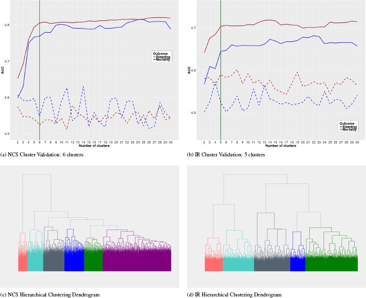
NCS and IR Data Cluster Validation and Dendrograms (dotted lines indicates performance for randomly generated clusters).

Random Forest Feature Contributions

An important component of the RF algorithm is its capability to produce a variable ranking score or variable importance based on association of a given predictor with other predictors and with the outcome variable. This score can help in interpretation of the model or for dimension reduction. The variable importance is a population measure, and as an average score, it does not indicate the relative influence of each patients’ feature value in predicting the outcome. A variable might be an important risk factor for the overall population, but not a risk factor for a given individual or subgroup of patients. Recently, the RF variable importance measure has been extended to an importance score or feature contribution¹⁹ for each individual patient in the training set. The feature contributions characterize the relative contribution of a patient’s baseline variables towards predicting an outcome value or class. Another attractive property of the feature contribution method is that it can be predicted for new patients. This offers a way to further validate the random forest model: when the average feature contributions of the training and test set matches, then the model can generalize well. For classification problems, a zero value for feature contribution indicates that the variable is irrelevant with respect to assigning a patient to a given class. Positive values indicate that the variable is influential towards classifying the patient to a reference class.

Treatment Effect of Plasma Transfusion

The standard approach to investigate the causal relationship between a treatment or exposure and an outcome is to construct statistical regression models in which the outcome is regressed against baseline covariates and the treatment variable. The attributable effect of the treatment is then read off as the corresponding regression coefficient. This study takes a different approach and estimates the treatment effect through application of machine learning methods. The theory of causal inference or technical details of the considered estimation procedure are beyond the scope of this study. The interested reader is referred to^16;24;25 for more details. However, for the purposes of this study, a brief discussion of the data structure required to compute these estimators is presented next.

Data structure and likelihood. The observations for each patient in the data set can be written as O = (X, Y, Z) where Z ∈ {0,1} is the treatment indicator with Z = 1 if patient was treated and Z = 0 if patient was not treated. X is a vector of baseline covariates that records information specific to each patient prior to treatment. Y is the outcome such as bleeding or mortality. The relationship between the observed variables in O can be written in a factorize data likelihood as

$$\mathrm{Pr}\left(X,Y,Z\right)=\stackrel{g}{\overbrace{\mathrm{Pr}\left(Z|X\right)}}\stackrel{Q}{\overbrace{\mathrm{Pr}\left(Y|X,Z\right)\mathrm{Pr}\left(X\right)}}$$ (1)

Pr(X) and Pr(Y|X, Z) are referred to as the Q component of the likelihood while Pr(Z|X) is the g component. g(Z|X) represents the propensity or the causal disposition of the treatment to produce some outcome. Let Q_o(Z, X) = E[Y|Z, X] be the true potential outcome conditional on the observed characteristics. Estimates of g and Q₀ can be obtained by standard regression or machine learning methods.

For a binary outcome and in the presence of no confounding variables, the treatment effect can be easily computed by taking the expectations ψ₁ = E[Y_Z=1] and ψ₀ = E[Y_Z=₀], where E[Y_Z=1] is the mean of Y assuming every patient in the population was exposed at level Z = 1. These two statistics can then be combined in useful ways to assess the effect of different levels of the treatment. Two commonly reported summary statistics include the Additive Treatment Effect: ATE = ψ₁ - ψ₀ and the Risk Ratio: RR = ψ₁/ψ₀.

The ATE quantifies the additive effect of every patient being exposed to the event versus not being exposed. Thus, a meaningful interpretation of ATE = 0.05 could read: “offering a patient plasma transfusion versus not increases the risk of bleeding/mortality by 5%”.¹⁶ The RR quantifies the multiplicative effect of being exposed versus not. A RR of 5 can be interpreted as: “offering a patient plasma transfusion versus not would lead to a 5 times increase in the risk of bleeding/mortality”.

Targeted maximum likelihood estimation. In observational studies, estimators of treatment effect need to account for possible confounding, i.e situations where the (apparent) effect of the treatment is actually the effect of another characteristic that is associated with both the treatment and the outcome. Several methods have been proposed for the estimation of ATE and RR in a way that can mitigate the effects of confounding (and model misspecification), e.g. G-computation formula, propensity score matching, inverse probability of treatment weighting (IPTW), and doubly-robust estimation. See^24;25 for more in-depth discussion of these estimators. In this study, the targeted maximum likelihood estimation (TMLE)^16;17 method is considered because of its double robustness and bias reduction properties. TMLE is a two stage doubly robust semi-parametric estimation methodology designed to minimize the bias of the parameters of interest. The first stage of the method estimates the density of the data generating distribution (specifically Q₀) while the second stage solves an efficient influence curve estimating equation. The influence curve describes the behavior of the target parameter under slight changes of the initial density estimates.

In TMLE, if either g or Q0 are consistently estimated, then the TMLE estimator is guaranteed to be asymptotically unbiased. However, TMLE will not return consistent estimates of the parameter of interest when both g and Q0 are misspecified. Thus it is important to avoid overfitting these measures.

As discussed above, estimating the two statistics ψ₁ and ψ₀ allows for calculating any of the causal effects ATE and RR. The TMLE estimate of ψ_z (z ∈ {0,1}) is given by

$${\widehat{\psi }}_z=\frac{1}{n}{\displaystyle \sum _{i=1}^n{\widehat{Q}}_0^{*}}(z,x_i)$$ (2)

where ${\widehat{Q}}_0^{\ast }(z,x_i)$is an update of ${\widehat{Q}}_0(z,x_i)$ The targeting step for updating ${\widehat{Q}}_0(z,x_i)$ is done by fluctuating ${\widehat{Q}}_0(z,x_i)$ through a parametric sub-model of the form: $logit\left({\widehat{Q}}_0^{*}\left(z,x\right)\right)=logit\left({\widehat{Q}}_0\left(z,x\right)\right)+Î{\widehat{H}}_z\left(z,r\right)$ where ∈ is the fluctuation parameter, $Î{\widehat{H}}_z\left(z,r\right)=I\left(Z=z\right)/\widehat{g}\left(z,x\right)$ is the efficient influence curve equations, and I is the indicator function. The MLE of ɛ is obtained by a logistic regression of Y on ${\widehat{H}}_z\left(z,r\right)$ with offset $logit\left({\widehat{Q}}_0\left(z,x\right)\right)$. Confidence intervals and p-value for TMLE can be obtained through the variance of the influence curve.

TMLE can use initial estimates of Q₀ and g from any fixed parametric model such as generalized linear models (GLM) (e.g logistic regression). However, most parametric models require a functional form for the predictors, and some assume distributions for the outcome and predictors variables, which are often not realistic such that model misspecification is difficult to avoid. It is therefore recommended to used machine learning methods that makes little or no assumptions and are able to estimate complex relationships between the outcome and observed variables.

Results

This section presents the main results: estimates of treatment effect of PPT on bleeding and mortality for the complete data and for each subgroup. For the calculations of ATE and RR, we estimate Q₀ and g using five models: generalized boosting machine (GBM), random forest, support vector machine (SVM), logistic regression and extreme logistic regression (ELR)²⁶ and select the best model through 5-fold cross-validation. First we present the cluster validation analysis, then the treatment effect analysis, and end the section with analysis of the population or median feature contributions over all patients in the cohort and the individual feature contributions for two random patients.

Cluster validation and selection of optimal number of clusters

A robust and stable clustering procedure generates homogeneous clusters such that patients within clusters are similar with respect to baseline characteristics. This implies the procedure has identified hidden structure in the data. A way to determine if the URF method identified underlying structure in the NCS and IR datasets is to look at the OOB error rates. Specifically, the OOB error rate for the NCS and IR data clustering problems were 11.95% and 1.20% respectively, indicating that the synthetic data destroyed existing structure in the data and the RF model was able to capture this information with high accuracy.

Ward’s Minimum Variance: URF can identify structure in the data, but obtaining good clusters crucially depends on the clustering algorithm. We employ the agglomerative hierarchical clustering algorithm with the Ward’s minimum variance criterion. Figure 1 (c) and (D) shows the dendrogram of the algorithm for the NCS and IR data sets respectively. The dendrogram represents the similarity relationships between patients in a tree-like form. Agglomerative hierarchical clustering starts by assuming that each patient is a cluster, and successively merges similar clusters to form larger clusters. Because of the hierarchical structure, different number of clusters can be obtained by cutting the tree at different heights. We used the Ward’s method, which minimizes the sums of squares between clusters to merge similar clusters together. However, we also tried other merging algorithms such as the single, complete, and average linkage methods, but all produced unstable and sparse clusters. In contrast, the Ward’s method produced stable and equal sized clusters.

Predictive Ability of Cluster Memberships: The clustering partitioned the data space into non-overlapping regions, where each region is associated to a given level of the treatment and outcome. In other words, if the regions are sufficiently homogeneous, then similar outcomes are expected for patients if offered the same treatment. As a consequence, a classification model can efficiently discriminate between the classes based on treatment status and subgroup allocations, and the discriminative power increases the more homogeneous the groups become.

Figure 1 (a) and (b) shows AUCs (averaged over 5-fold cross-validation) of a logistic regression model predicting bleeding (red curve) and mortality (blue curve) based on cluster memberships and plasma transfusion plotted against the number of clusters. Clearly, the cluster memberships are predictive as can be seen by the rise in AUC as the number of clusters increases (solid lines) compared to the poor and unstable performance of a randomly generated clusters (dotted lines). There is a big jump in performance from 2, 3 and 4 clusters to 5 or 6 clusters. After the 5’th or 6’th cluster, the relative increase in AUC reduces and becomes somewhat stable. We choose the number of clusters as that corresponding to the elbow or turning point of the curve. At the elbow, adding another cluster to the logistic regression model does not lead to any appreciable performance gain. Thus, 6 clusters are optimal for the NCS data and 5 for IR. Close observation of the curves will indicate that 7 or 8 clusters can equally be selected. However, these higher cluster numbers produced very sparse distributions of the observed treatment and outcome events in some of the clusters. In our implementation, we set the minimum number of events observed in each cluster to 10.

Effect of Plasma Transfusion on Bleeding and Mortality

Population Effect: Table 1 presents the ATE and RR quantifying the population effect of PPT on bleeding and mortality for the NCS and IR datasets. The GBM algorithm performed best for the NCS data, while the ELR offered the best

performance for the IR data. To save on space, discussions will be restricted to the ATE summary statistics; interpretations for RR can be similarly made. Overall, the estimates from TMLE confirmed previous findings that population wise, PPT increases the risk of bleeding.^8;27 Specifically, for the population of NCS and IR patients considered in this study, PPT significantly increases the risk of bleeding by 14% (p-value = 0.00) and 12% (p-value = 0.00) respectively (95% confidence intervals are shown in brackets). With respect to mortality, PPT marginally increases risk by 4% for NCS and has no effect for IR populations.

Subgroup Effect: Table 2 presents estimates of ATE and RR within each cluster identified for the NCS and IR data sets. With respect to the NCS clusters, we found: (a) One cluster with 551 patients where PPT increases the risk of bleeding and mortality by 32% and 6% (p-value = 0.00 and 0.05) respectively. (b) One cluster where PPT has no effect on bleeding and mortality. This cluster may represent patients where the administration of prophylactic plasmatransfusion is wasteful. (c) Two clusters of sizes 150 and 127, where PPT reduces the risk of bleeding by 9% in each cluster. Correspondingly, PPT increases the risk of mortality in one cluster and has no effect in the second. (d) The last cluster with 171 patients show harmful effect of PPT on bleeding and no effect on mortality.

Overall, the effect PPT on bleeding for the NCS data was beneficial in two subgroups and none showed any beneficial effect with respect to mortality. It is therefore interesting to investigate the characteristics of patients in these subgroups. This information can help reduce the inappropriate use of plasma products as only the patients who will truly benefit from plasma transfusion are considered for treatment.

For the IR data clustering, we found roughly similar results. One group with 187 patients having beneficial effect of PPT on bleeding (11%, p-value=0.00). The IR data set however contains two subgroups with beneficial effect of PPT on mortality. The NCS and IR clustering problems contains subgroups (n = 75 and 451 respectively) where the observed number of patients with bleeding/mortality and PPT events was less than 10, and no treatment effect estimates were computed for these groups.

Feature Contributions

We report only the results for the NCS complete data. Result for the IR data and all subgroups can be obtained by contacting the authors. Figures 2 (a) and (b) shows the median feature contributions for all patients averaged over five-fold cross-validation and the corresponding feature contributions for two random patients. The two patients (P1 and P2) were both offered plasma transfusion but experience different levels of the bleeding/mortality outcome: P1 bled/died and P2 did not bleed/die. Preoperative hemoglobin levels and PLT test value (platelet count) are the two most contributing variables towards predicting bleeding and mortality. Though appearing in different order, the same 9 variables appear among the top 10 most predictive variables for all patients in the two models. Considering the median feature contribution, these top 9 variables are somewhat equally contributive towards predicting whether a patient will bleed or not. However, these variables contribute more towards predicting the death status of a patient compared to predicting alive status.

Figure 2.

Top 35 features contributions towards predicting Bleeding and Mortality (NCS data)

The plots clearly show that significant variabilities exist between population level (median) feature contributions and the individual level. For example, while plasma transfusion is a strong contributing factor towards predicting bleeding for the random patients, the effect of the variable is almost zero when we consider the population level. Similarly, while the population level contributing factor of connective tissue disease is almost zero, it however contributes significantly towards predicting the death status of the random patient P1.

Conclusion

The most common reason cited for plasma transfusion is the correction of an elevated pre-operation/pre-procedural international normalized ratio (INR) for the prevention of bleeding complications,^4;10 despite lack of evidence to support such practices. The decision to offer plasma transfusion to patients with abnormal coagulation factors still remains largely controversial. Current recommendations are mostly based on expert opinion and a precautionary approach to correct abnormal laboratory tests results and there is wide spread variation in the practice with respect to plasma transfusion.^2–4 Many studies, including randomized control trials have shown no significant benefit for prophylactic and therapeutic use of fresh frozen plasma (FFP) across a range of indications.^3;4;28 Moreover, majority of these studies report the inappropriateness and harmful effect of prophylactic plasma transfusion. However, almost all the studies have evaluated the effect of plasma transfusion at the population level. Despite accounting for parameters such as treatment selection bias and potential confounding in observational studies, those results apply essentially to the average patient. Given that the critically ill patient population can be highly heterogeneous in their responses to treatments, the average effect of a treatment is of limited value, as it ignores individual patient level variabilities of the treatment, which often deviate substantially from the population average. Furthermore, except for the work in,⁸ most of the published work on the effect of plasma transfusion have traditionally used classical regression, propensity score, and matching methods, which often make unrealistic and difficult to satisfy assumptions about the patient population.

This study takes a different approach and applied subgroup analysis based on efficient and robust machine learning methods and identified several homogeneous subgroups exhibiting differential effects of plasma transfusion on bleeding and mortality. Specifically, using the unsupervised random forest (URF)^13;21 clustering method and the doubly robust targeted maximum likelihood estimation (TMLE) method,¹⁷ we identified stabled and clinically meaningful subgroups with beneficial, harmful, and no effect of plasma transfusion on bleeding and mortality. Recognizing the widespread inappropriate use of FFP and the lack of evidence to support the use of plasma transfusion to prevent bleeding, the results from this study suggest that researchers should reconsider evaluation measures based on the overall population, and strongly support the fact that blood transfusion therapy should be customized for the individual patient. Further, analysis of the subgroup characteristics can help shed light on the much needed evidence to support the use of plasma transfusion to correct prolonged prothrombin time and prevention of bleeding complications.

Table 1:

Population Effect of PPT on Bleeding and Mortality

Data	Outcome	ATE	p-value	RR	p-value
NCS	Bleeding	0.14 (0.08, 0.20)	0.00	1.438 (1.25, 1.65)	0.00
	Mortality	0.04 (0.00, 0.09)	0.00	1.523 (1.06, 2.00)	0.02
IR	Bleeding	0.12 (0.09, 0.15)	0.00	2.01 (1.68, 2.39)	0.00
	Mortality	-0.01 (-0.03, 0.02)	0.53	0.92 (0.72, 1.19)	0.54

Table 2:

Subgroup Effects of PPT on Bleeding and Mortality

Data	Cluster		ATE	p-value	RR	p-value
NCS	Cluster 1 (n=171)	Bleeding	-0.02 (-0.11,0.08)	0.73	0.98 (0.84, 1.13)	0.74
		Mortality	-0.03 (-0.12, 0.06)	0.53	0.89 (0.60, 1.30)	0.53
	Cluster 2 (n=551)	Bleeding	0.32 (0.23, 0.41)	0.00	2.06 (1.71, 2.47)	0.00
		Mortality	0.06 (0.00, 0.13)	0.05	1.67 (1.08, 2.59)	0.02
	Cluster 3 (n=150)	Bleeding	-0.09 (-0.18, -0.01)	0.04	0.49 (0.21, 1.11)	0.09
		Mortality	0.74 (0.65, 0.82)	0.00	26.26 (10.07, 68.48)	0.00
	Cluster 4 (n=171)	Bleeding	0.13 (0.06, 0.20)	0.00	2.22 (1.42, 3.49)	0.00
		Mortality	-0.01 (-0.02, 0.01)	0.30	0.00 (0.00, 0.00)	0.00
	Cluster 5 (n=127)	Bleeding	-0.09 (-0.12, -0.04)	0.001	0.00 (0.00, 0.00)	0.00
		Mortality	-0.01 (-0.02, 0.01)	0.32	0.00 (0.00, 0.00)	0.00
	Cluster 6 (n=75)	Bleeding	-	-	-	-
		Mortality	-	-	-	-
IR	Cluster 1 (n=650)	Bleeding	0.37 (0.33, 0.42)	0.00	4.92 (3.75, 6.44)	0.00
		Mortality	-0.04 (-0.07, -0.01)	0.02	0.60 (0.39, 0.92)	0.02
	Cluster 2 (n=390)	Bleeding	0.06 (-0.01, 0.13)	0.11	1.45 (0.94, 2.23)	0.09
		Mortality	0.01 (-0.06, 0.07)	0.89	1.038 (0.62, 1.75)	0.90
	Cluster 3 (n=451)	Bleeding	-	-	-	-
		Mortality	-	-	-	-
	Cluster 4 (n=224)	Bleeding	0.12 (0.03, 0.21)	0.01	1.50 (1.11, 2.03)	0.01
		Mortality	-0.11 (-0.18, -0.04)	0.002	0.47 (0.28, 0.81)	0.01
	Cluster 5 (n=187)	Bleeding	-0.11 (-0.18, -0.04)	0.003	0.49 (0.29, 0.81)	0.01
		Mortality	0.02 (-0.06, 0.10)	0.62	1.11 (0.73 1.70)	0.62

References

- 1.Malloy PC, Grassi CJ, Kundu S, Gervais DA, Miller DL, Osnis RB, et al. Standards of practice committee with cardiovascular and interventional radiological society of europe (cirse) endorsement. consensus guidelines for periprocedural management of coagulation status and hemostasis risk in percutaneous image-guided interventions. J Vasc Interv Radiol. 2009;20(7) doi: 10.1016/j.jvir.2008.11.027. [DOI] [PubMed] [Google Scholar]
- 2.Arnold Donald M, Lauzier Francois, Whittingham Heather, Zhou Qi, Crowther Mark A, McDonald Ellen, et al. A multifaceted strategy to reduce inappropriate use of frozen plasma transfusions in the intensive care unit. Journal of critical care. 2011;26(6):636–e7. doi: 10.1016/j.jcrc.2011.02.005. [DOI] [PubMed] [Google Scholar]
- 3.Gorlinger Klaus, Saner Fuat H. Prophylactic plasma and platelet transfusion in the critically ill patient: just useless and expensive or even harmful? BMC anesthesiology. 15(1):86, 2015. doi: 10.1186/s12871-015-0074-0. [DOI] [PMC free article] [PubMed] [Google Scholar]
- 4.Hall DP, Lone NI, Watson DM, Stanworth SJ, Walsh TS. (of Coagulopathy (ISOC) Investigators Intensive Care Study), et al. Factors associated with prophylactic plasma transfusion before vascular catheterization in non-bleeding critically ill adults with prolonged prothrombin time: a case-control study. British journal of anaesthesia. 2012;109(6):919–927. doi: 10.1093/bja/aes337. [DOI] [PubMed] [Google Scholar]
- 5.MozesMD B, Epstein M, Ben-Bassat I, Modan B, Halkin H. Evaluation of the appropriateness of blood and blood product transfusion using preset criteria. Transfusion. 1989;29(6):473–476. doi: 10.1046/j.1537-2995.1989.29689318442.x. [DOI] [PubMed] [Google Scholar]
- 6.Li Guangxi, Rachmale Sonal, Kojicic Marija, Shahjehan Khurram, Malinchoc Michael, Kor Daryl J, et al. Incidence and transfusion risk factors for transfusion-associated circulatory overload among medical intensive care unit patients. Transfusion. 2011;51(2):338–343. doi: 10.1111/j.1537-2995.2010.02816.x. [DOI] [PMC free article] [PubMed] [Google Scholar]
- 7.Watson Gregory A, Sperry Jason L, Rosengart Matthew R, Minei Joseph P, Harbrecht Brian G, Moore Ernest E, et al. Fresh frozen plasma is independently associated with a higher risk of multiple organ failure and acute respiratory distress syndrome. Journal of Trauma and Acute Care Surgery. 2009;67(2):221–230. doi: 10.1097/TA.0b013e3181ad5957. [DOI] [PubMed] [Google Scholar]
- 8.Ngufor C, Murphree D, Upadhyaya S, Madde N, Kor D, Pathak J. Effects of plasma transfusion on perioperative bleeding complications: A machine learning approach. Studies in health technology and informatics. 2015;216:721. [PMC free article] [PubMed] [Google Scholar]
- 9.Jia Qing, Brown Michael J, Clifford Leanne, Wilson Gregory A, Truty Mark J, Stubbs James R, et al. Prophylactic plasma transfusion for surgical patients with abnormal preoperative coagulation tests: a single-institution propensity-adjusted cohort study. The Lancet Haematology. 2016;3(3):e139–e148. doi: 10.1016/S2352-3026(15)00283-5. [DOI] [PMC free article] [PubMed] [Google Scholar]
- 10.Warner Matthew A, Woodrum David A, Hanson Andrew C, Schroeder Darrell R, Wilson Gregory A, Kor Daryl J. In Mayo Clinic Proceedings. Vol. 91. Elsevier; 2016. Prophylactic plasma transfusion before interventional radiology procedures is not associated with reduced bleeding complications; pp. 1045–1055. [DOI] [PMC free article] [PubMed] [Google Scholar]
- 11.Davidoff Frank. Heterogeneity is not always noise: lessons from improvement. Jama. 2009;302(23):2580–2586. doi: 10.1001/jama.2009.1845. [DOI] [PubMed] [Google Scholar]
- 12.Ruberg Stephen J, Chen Lei, Wang Yanping. The mean does not mean as much anymore: finding sub-groups for tailored therapeutics. Clinical trials. 2010 doi: 10.1177/1740774510369350. [DOI] [PubMed] [Google Scholar]
- 13.Breiman Leo. Random forests. Machine learning. 2001;45(1):5–32. [Google Scholar]
- 14.Rosenbaum Paul R, Rubin Donald B. The central role of the propensity score in observational studies for causal effects. Biometrika. 1983;70(1):41–55. [Google Scholar]
- 15.Faries Douglas E, Chen Yi, Lipkovich Ilya, Zagar Anthony, Liu Xianchen, Obenchain Robert L. Local control for identifying subgroups of interest in observational research: persistence of treatment for major depressive disorder. International journal of methods in psychiatric research. 2013;22(3):185–194. doi: 10.1002/mpr.1390. [DOI] [PMC free article] [PubMed] [Google Scholar]
- 16.Van der Laan Mark J, Rose Sherri. Targeted learning: causal inference for observational and experimental data. Springer; 2011. [Google Scholar]
- 17.Gruber Susan, van der Laan Mark J. tmle: an r package for targeted maximum likelihood estimation. 2011 [Google Scholar]
- 18.Herasevich V, Kor DJ, Li M, Pickering BW. Icu data mart: a non-it approach. a team of clinicians, researchers and informatics personnel at the mayo clinic have taken a homegrown approach to building an icu data mart. Healthcare informatics: the business magazine for information and communication systems. 2011;28(11):42–44. [PubMed] [Google Scholar]
- 19.Palczewska Anna, Palczewski Jan, Robinson Richard Marchese, Neagu Daniel. In Integration of Reusable Systems. Springer; 2014. Interpreting random forest classification models using a feature contribution method; pp. 193–218. [Google Scholar]
- 20.Stekhoven Daniel J, Buhlmann Peter. Missforest—non-parametric missing value imputation for mixed-type data. Bioinformatics. 2012;28(1):112–118. doi: 10.1093/bioinformatics/btr597. [DOI] [PubMed] [Google Scholar]
- 21.Shi Tao, Horvath Steve. Unsupervised learning with random forest predictors. Journal of Computational and Graphical Statistics. 2006;15(1):118–138. [Google Scholar]
- 22.Afanador Nelson Lee, Smolinska Agnieszka, Tran Thanh N, Blanchet Lionel. Unsupervised random forest: a tutorial with case studies. Journal of Chemometrics. 2016;30(5):232–241. [Google Scholar]
- 23.Tan Pang-Ning. Pearson Education India. Introduction to data mining. 2006 [Google Scholar]
- 24.Hubbard Alan E, Van Der Laan Mark J. Population intervention models in causal inference. Biometrika. 2008;95(1):35–47. doi: 10.1093/biomet/asm097. [DOI] [PMC free article] [PubMed] [Google Scholar]
- 25.Young Jessica G, Hubbard Alan E, Eskenazi B, Jewell Nicholas P. A machine-learning algorithm for estimating and ranking the impact of environmental risk factors in exploratory epidemiological studies. 2009 [Google Scholar]
- 26.Ngufor Che, Wojtusiak Janusz. Extreme logistic regression. Advances in Data Analysis and Classification. 2014:1–26. [Google Scholar]
- 27.Jacob Laurent, Vert Jean-philippe, Bach Francis R. Clustered multi-task learning: A convex formulation. In Advances in neural information processing systems. 2009:745–752. [Google Scholar]
- 28.Stanworth SJ, Brunskill SJ, Hyde CJ, McClelland DBL, Murphy MF. Is fresh frozen plasma clinically effective? a systematic review of randomized controlled trials. British journal of haematology. 2004;126(1):139–152. doi: 10.1111/j.1365-2141.2004.04973.x. [DOI] [PubMed] [Google Scholar]