Tracking Non-stationary EEG Sources using Adaptive Online Recursive Independent Component Analysis

Abstract

Electroencephalographic (EEG) source-level analyses such as independent component analysis (ICA) have uncovered features related to human cognitive functions or artifactual activities. Among these methods, Online Recursive ICA (ORICA) has been shown to achieve fast convergence in decomposing high-density EEG data for real-time applications. However, its adaptation performance has not been fully explored due to the difficulty in choosing an appropriate forgetting factor: the weight applied to new data in a recursive update which determines the trade-off between the adaptation capability and convergence quality. This study proposes an adaptive forgetting factor for ORICA (adaptive ORICA) to learn and adapt to non-stationarity in the EEG data. Using a realistically simulated non-stationary EEG dataset, we empirically show adaptive forgetting factors outperform other commonly-used non-adaptive rules when underlying source dynamics are changing. Standard offline ICA can only extract a subset of the changing sources while adaptive ORICA can recover all. Applied to actual EEG data recorded from a task-switching experiments, adaptive ORICA can learn and re-learn the task-related components as they change. With an adaptive forgetting factor, adaptive ORICA can track non-stationary EEG sources, opening many new online applications in brain-computer interfaces and in monitoring of brain dynamics.

I. INTRODUCTION

A variety of analytical tools for biosignals such as EEG have successful uncovered functional features related to human cognitive functions and non-brain activities [1]. In order to obtain robust estimates from noisy measurements, most of the analyses are done offline and assuming stationary data. However, in practical applications such as brain-computer-interfaces and clinical monitoring of brain dynamics, batch learning is rather infeasible in the online environment due to the large number of samples required and high computational load [2]. Furthermore, assumptions of stationarity often do not apply to real-life situations, where humans organize their behavior with respect to a complex, multi-scale and ever-changing environment. Therefore, EEG source activities are inevitably non-stationary.

To address this, several online learning methods have been proposed which take into account non-stationarity in the data to study brain dynamics or mitigate non-stationarity problem [2][3][4]. Among these methods, Akhtar et al. [5] have proposed Online Recursive ICA (ORICA), derive from iterative inversion of the fixed point solution to natural gradient Infomax ICA rule, yielding the fast convergence of a recursive-least-squares (RLS) type filter and low computational load. Previous studies have shown that ORICA is capable of real-time processing of high-density EEG data and extracting informative sources from experimental EEG data comparable to those of standard ICA approaches [6][7]. However, one important advantage of online ICA—adaptation performance—has not been explored. The difficulty lies in choosing a forgetting factor: the weight applied to new data in a recursive update rule determining the tradeoff between adaptation capability and convergence quality.

This study proposes an adaptive forgetting factor for ORICA (adaptive ORICA), modified from the adaptive rule of [2] and [8], to learn and adapt to the non-stationary data. To compare the performance of adaptive and non-adaptive forgetting factors, we use a realistically simulated non-stationary EEG dataset with the underlying sources activating and deactivating alternatively. We also compare the results of adaptive ORICA to those of a standard offline ICA (Infomax) [1]. Finally, we demonstrate the real-world applicability of adaptive ORICA using 14-ch EEG data recorded from a subject performing a task-switching experiment.

II. Methods

A. Online recursive ICA (ORICA)

With the assumption that scalp EEG signals (x) are linear mixtures of underlying independent sources (s), i.e. x = As, ICA aims to learn an unmixing matrix B such that the estimated source activations y are recovered, with permutation and scaling ambiguities, by y = Bx.

An online framework is proposed which separates the unmixing process into two stages B = WM [6]. The whitening matrix M is updated by an online RLS whitening update [9] to decorrelate the signals:

$$M_{n+1}=M_n+\frac{{\lambda }_n}{1-{\lambda }_n}\left[I-\frac{v_n·v_n^T}{1+{\lambda }_n(v_n^T·v_n-1)}\right]M_n,$$ (1)

where v_n = M_nx_n are the decorrelated signals and λ_n is a time-varying forgetting factor. This is followed by ORICA update on the weight matrix W [5]:

$$W_{n+1}=W_n+\frac{{\lambda }_n}{1-{\lambda }_n}\left[I-\frac{y_n·f_n^T}{1+{\lambda }_n(f_n^T·y_n-1)}\right]W_n$$ (2)

where y_n = W_nv_n are the recovered source activations and f(y) = −2 tanh(y) are the component-wise nonlinear functions for super-gaussian sources and f(y) = tanh(y) − y for sub-gaussian sources. An orthogonalization step is applied after each update to ensure W matrix remains orthogonal. Following [6], we assume all EEG sources are super-gaussian to improve convergence and we concurrently update the M and W matrix for a block of samples (here we used 8 samples to a block) to reduce the computational load. The forgetting factors in equations 1 and 2 are chosen to be the same.

B. Adaptive forgetting factor

In adaptive RLS filtering, the forgetting factor λ determines the effective length for a time window wherein data are exponentially weighted. A small value of λ corresponds to a long window length which yields small errors and good stability at the expense of tracking capability [10].

Three update rules for forgetting factors are considered: constant, monotonically decreasing (cooling), and adaptive. In a conventional RLS filter, a constant forgetting factor rule is often used so that it has moderate tracking performance, but the error at convergence can be large. In order to achieve better learning performance, it is desirable to have a large λ during initial learning to increase convergence speed and a small λ near convergence to minimize error. To this end, a cooling forgetting factor may lead to satisfactory performance. We use the rule defined in [11] as ${\lambda }_n=\frac{{\lambda }_0}{n^{\gamma }}$, where λ₀ is the initial forgetting factor and γ determines its decay rates. The convergence rate of the cooling scheme is analyzed in [12]. Despite the good convergence, the annealed λ cannot follow non-stationarity in the data. Clearly, there is a need for an adaptive forgetting factor which increases during the presence of non-stationarity and otherwise decreases for fast and stable convergence.

To realize an adaptive forgetting factor, we need to quantify the non-stationarity in the data. Since ORICA is derived from the fixed point solution of minimizing <I − yf^T>, the non-stationarity can be assessed by the error of nonlinear decorrelation, i.e. $I-y_n{f}_n^T$. To increase the robustness of the estimates, a leaky average with weight δ is used:

$$R_{n+1}=(1-\delta )R_n+\delta (I-y_n{f}_n^T)$$ (3)

The final non-stationarity index z_n is a scalar indicator of convergence for all sources which is defined as:

$$z_n={\Vert R_n\Vert }_F$$ (4)

Motivated by Murata et al. [2], we use the following adaptive forgetting factor:

$${\lambda }_{n+1}={\lambda }_n-\alpha {\lambda }_n^2+\beta G(z_{n+1}){\lambda }_n$$ (5)

where α controls the decay rate of λ in the learning stage (when data are relatively stationary) and β sets an upper bound on how fast λ can increase during the tracking stage (when data are non-stationary). In [2], the βG(z) term in equation (5) is defined as z_n/z_max. However, the linear mapping between z_n and λ_n does not work effectively when data dimension increases due to a large initial value of z.

To address the issue, inspired by the synaptic update from [8], we design G(z) as a modified tanh function which maps the non-stationarity index z_n to a value from 0 to 1 indicating the level of λ adjustment:

$$G(z)=\frac{1}{2}\left\{1+tanh\left[\frac{1}{b}(\frac{z}{max(z_{\mathit{min}},\epsilon )}-c)\right]\right\}$$ (6)

where b and c determine the bandwidth and the center of the tanh function. The term z_min is an indicator for initial convergence and ε controls the switching from learning stage to tracking stage. In the learning stage, we want G(z) to be small so that λ can decrease to a small value to ensure convergence. In the tracking stage, we want G(z) to be large when non-stationarity index increases.

Although many parameters are introduced in equation 5, Murata et al. [2] have discussed how to choose α, β and δ. As for b and c in equation 6, they can be designed according to the mean and variance of the non-stationarity index. This study follows the principles to search for optimal parameters.

III. Materials

A. Data collection

1) Simulated EEG data

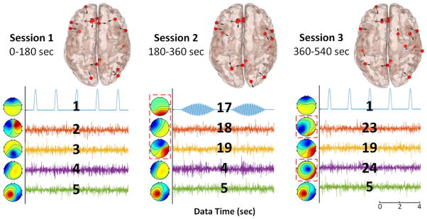
We simulate a realistic form of non-stationarity in the EEG data where the underlying sources in the brain are activating and deactivating alternately, using the EEG simulator in Source Information Flow Toolbox (SIFT) [1]. We first generate source time-series using a random-coefficient stationary autoregressive models with super-gaussian noises (128Hz sampling rate, nine minutes). In addition, two sources simulating eye blinks and alpha burst activities are manually designed (source #1 and #17 in Fig. 1). Each source is assigned to the center of a randomly selected cortical region from MNI brain atlas, with its dipole orienting normal to the cortical surface. Cortical regions for eye-blink and alpha components are manually selected to match reality (see head models in Fig. 1).

Fig. 1.

Source dipole locations and orientations (red dots and black arrows respectively in cortical head models), 10 second examples of source time-series, and component maps of select components in three sessions for the simulated 16-ch non-stationary EEG data. The red dashed boxes indicate which sources changed between sessions. Each source is labeled for comparisons with Fig. 3.

The nine minutes of source data are partitioned into three 3-min sessions, each with a different set of 16 selected (active) sources. Between each session, six sources are changed, including alternating between the eye-blink and alpha components, while ten sources remain the same. The active sources in each session are designed such that all simulated sources (27 in total) are active in at least one session. Finally, the source-level activities are projected through a zero-noise 3-layer Boundary Element Method (BEM) forward model (MNI Colin27), yielding 16-channel EEG data.

2) Actual EEG data

Three sessions of EEG data are collected from a 26 year-old male subject using a 14-channel wearable wireless Emotiv headset. The first and third session are 3-min eye-closed music listening, and the second session is 3-min eye-open typing, with ten second transitions between sessions. Artifact Subspace Reconstruction (ASR) [13], an online-capable method to detect and repair temporal burst artifacts based on signals’ covariance, is applied prior to online ICA pipeline. Our goal is to see the switching of active sources in each session.

B. Data processing

For running adaptive ORICA, both simulated and actual EEG data are processed in a simulated online environment using BCILAB [14]. The online ICA pipeline consists of an IIR high-pass filter (cutoff at 1Hz), an online RLS whitening filter, and an ORICA filter. As a comparison, we also apply a standard batch mode ICA (Infomax) available in EEGLAB [1] to both simulated and actual EEG datasets. Note that the Infomax ICA is performed on whole datasets instead of on data in each session.

IV. Results

A. Simulated 16-ch non-stationary EEG data

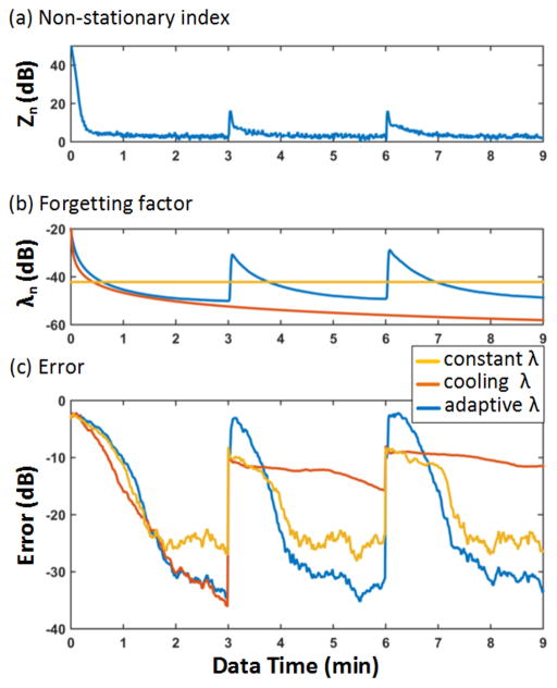
Fig. 2 demonstrates the learning and tracking performance of ORICA with three types of forgetting factors. The performance is quantified as the cross-talk error in Fig. 2c, which is a measurement of ICA decomposition given the ground truth as defined in equation (5) in [6]. The error zero implies perfect source separation, except for permutation and scaling ambiguities.

Fig. 2.

Time evolution of (a) the non-stationarity index z_n, (b) the forgetting factor λ_n, and (c) cross-talk error of ORICA decompositions with adaptive, cooling, and constant forgetting factor profiles applied to the simulated EEG data. Parameters are defined belows: for constant case, λ = 0.0078; for cooling case, λ_n = 0.995/n^0.6, for adaptive case, λ₀ = 0.1, α = 0.03, β = 0.012, δ = 0.05, b = 1.5, c = 5.

In the initial learning stage (0 to 3 minute), adaptive and cooling forgetting factors can achieve smaller errors comparing to the constant λ. In the tracking stage (3 to 9 minute), the non-stationarity index can successfully detect when the underlying sources change between sessions (Fig. 2a), which leads to an increase of the adaptive λs (Fig. 2b). This enables ORICA to relearn a new set of sources. The convergence speed after such a change is faster than that of the initial learning and reaches a comparable error level to previous sessions. Constant λ allows tracking to some extent; and while bigger λ values increase the convergence speed, they limit the quality of convergence. Cooling λs decline to values so small that tracking becomes impossible.

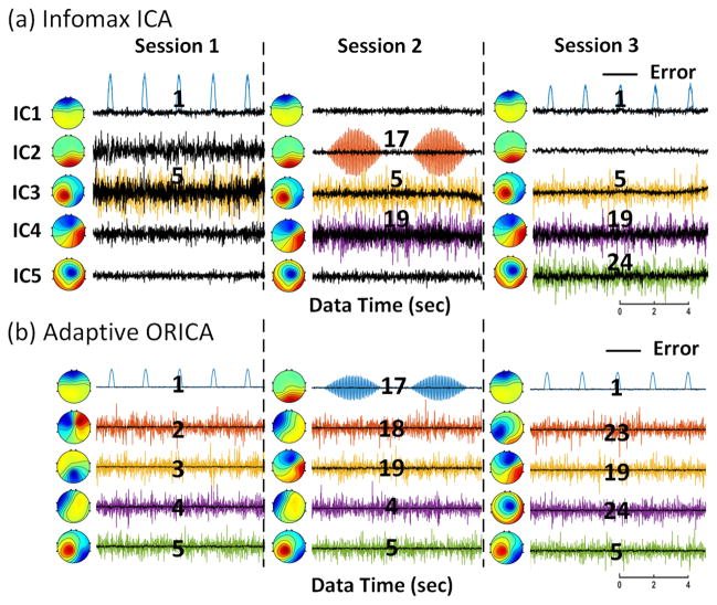
Fig. 3 shows that adaptive ORICA can separate all sources in each session while Infomax ICA can only extract a subset of the sources, as it is inherently an over-complete problem: the number of distinct sources (27) across three sessions is larger than the number of channels (16). Infomax ICA successfully decomposes the simulated eye-blink component (#1) which activates in sessions 1 and 3 while losing one dimension to account for a new source in session 2. Similarly, Infomax ICA finds the occipital alpha component (#17) which only activates in session 2, at the expense of missing sources in sessions 1 and 3. Other sources activating during different sessions are presented. The errors of Infomax ICA decompositions are near -10dB, as opposed to -30dB of adaptive ORICA.

Fig. 3.

Component maps of select sources corresponding to those in Fig. 1 (matched by correlation of component maps) decomposed and reconstructed by (a) Infomax ICA and (b) ORICA with an adaptive forgetting factor for the three sessions of simulated EEG data. 10 second windows of their reconstructed source time-series from the end of each session are presented. See Fig. 1 for an explanation of source numbering.

B. Actual 14-ch EEG data from the task-switching experiment

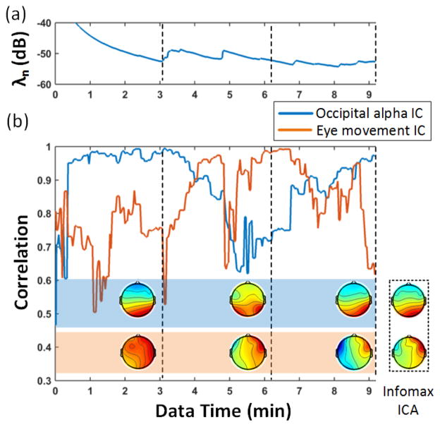
Fig. 4 demonstrates that adaptive ORICA can learn, forget, and relearn the task-specific sources in the task-switching experiment. In the first session (eye-closed), adaptive ORICA can quickly learn the alpha IC but not the eye-movement IC. In the second session (eye-open), the adaptive λ responds to the change of EEG sources at the transition between sessions (at 3 min 10 sec) and thus enables ORICA to learn the new eye-movement IC while gradually forgetting the alpha IC as it is not active anymore. Switching back to the eye-closed third session, adaptive ORICA can relearn the fading alpha IC and gradually lose the eye-movement IC. This demonstrates the applicability of adaptive ORICA to actual non-stationary EEG data. Note that some within-session non-stationarity is also present. Auditory and motor components are not clearly observed due to the limited scalp coverage of the Emotiv headset.

Fig. 4.

Adaptive ORICA applied to actual 14-ch EEG data from the task-switching experiment. Time evolution of (a) the adaptive forgetting factor and (b) the similarity (correlation) between two components decomposed by adaptive ORICA and Infomax ICA. The two components correspond to occipital alpha and horizontal eye movement activities. Dashed lines indicate the end of each session. The component maps solved by adaptive ORICA at the end of each session are shown to the left of the dashed lines with the component maps solved by Infomax ICA applied to the whole dataset are shown in a dashed box. Parameters used for adaptive ORICA: λ₀ = 0.1, α = 0.03, β = 0.005, δ = 0.05, b = 0.5, c = 3.

V. Conclusions

This study proposes and validates an adaptive forgetting factor update rule, which allows ORICA to adapt to changes in the underlying structure of the data. A realistically simulated EEG dataset mimicking brain sources activating and deactivating tests the performance of adaptive ORICA. Empirical results show that the adaptive rule maintains the fast and stable convergence of a cooling forgetting factor while presenting the ability to track changes when non-stationarity is detected. Standard offline ICA cannot solve the over-complete problem, while adaptive ORICA can learn the switching sources. Applied to actual EEG recorded from a task-switching experiment, we demonstrate adaptive ORICA can learn, forget, and relearn the task-related components.

Future works include (a) the development of an automatic, data-driven approach for selecting parameter values in the adaptive rule and (b) the integration of an online artifact removal method to stabilize ORICA convergence. The ability to track the changes in EEG source activities by the proposed method might lead to many real-world applications where modeling and tracking source dynamics are imperative.

References

- 1.Delorme A, Mullen T, Kothe C, Acar ZA, Bigdely-Shamlo N, Vankov A, Makeig S. Eeglab, sift, nft, bcilab, and erica: new tools for advanced eeg processing. Computational intelligence and neuroscience. 2011;2011:10. doi: 10.1155/2011/130714. [DOI] [PMC free article] [PubMed] [Google Scholar]
- 2.Murata N, Kawanabe M, Ziehe A, Müller K-R, Amari S-i. On-line learning in changing environments with applications in supervised and unsupervised learning. Neural Networks. 2002;15(4):743–760. doi: 10.1016/s0893-6080(02)00060-6. [DOI] [PubMed] [Google Scholar]
- 3.von Bunau P, Meinecke FC, Scholler S, Muller K. Finding stationary brain sources in eeg data. IEEE EMBS. 2010:2810–2813. doi: 10.1109/IEMBS.2010.5626537. [DOI] [PubMed] [Google Scholar]
- 4.Barlow JS. Methods of analysis of nonstationary eegs, with emphasis on segmentation techniques: a comparative review. Journal of Clinical Neurophysiology. 1985;2(3):267–304. doi: 10.1097/00004691-198507000-00005. [DOI] [PubMed] [Google Scholar]
- 5.Akhtar MT, Jung T-P, Makeig S, Cauwenberghs G. Recursive independent component analysis for online blind source separation. IEEE Circuits and Systems (ISCAS) 2012:2813–2816. [Google Scholar]
- 6.Hsu S-H, Mullen T, Jung T-P, Cauwenberghs G. Online recursive independent component analysis for real-time source separation of high-density eeg. IEEE EMBS. 2014:3845–3848. doi: 10.1109/EMBC.2014.6944462. [DOI] [PubMed] [Google Scholar]
- 7.Akhtar MT, Jung T-P, Makeig S, Cauwenberghs G. Validating online recursive independent component analysis on eeg data. IEEE EMBS Neural Engineering Conference; 2015. [Google Scholar]
- 8.Cichocki A, Unbehauen R. Robust neural networks with online learning for blind identification and blind separation of sources. IEEE Trans on Circuits and Systems I. Fundamental Theory and Applications. 1996;43(11):894–906. [Google Scholar]
- 9.Zhu X, Zhang X, Ye J. Natural gradient-based recursive least-squares algorithm for adaptive blind source separation. Science in China Series F: Information Sciences. 2004;47(1):55–65. [Google Scholar]
- 10.Paleologu C, Benesty J, Ciochina S. A robust variable forgetting factor recursive least-squares algorithm for system identification. Signal Processing Letters, IEEE. 2008;15:597–600. [Google Scholar]
- 11.Yin G. Adaptive filtering with averaging. Springer; 1995. [Google Scholar]
- 12.Amari S-I. Natural gradient works efficiently in learning. Neural computation. 1998;10(2):251–276. [Google Scholar]
- 13.Mullen T, Kothe C, Chi YM, Ojeda A, Kerth T, Makeig S, Cauwenberghs G, Jung T-P. Real-time modeling and 3d visualization of source dynamics and connectivity using wearable eeg. IEEE EMBS. 2013;2013:2184–2187. doi: 10.1109/EMBC.2013.6609968. [DOI] [PMC free article] [PubMed] [Google Scholar]
- 14.Kothe CA, Makeig S. Bcilab: a platform for brain–computer interface development. Journal of neural engineering. 2013;10(5):056014. doi: 10.1088/1741-2560/10/5/056014. [DOI] [PubMed] [Google Scholar]