Detecting Item Preknowledge Using a Predictive Checking Method

Abstract

Repeatedly using items in high-stake testing programs provides a chance for test takers to have knowledge of particular items in advance of test administrations. A predictive checking method is proposed to detect whether a person uses preknowledge on repeatedly used items (i.e., possibly compromised items) by using information from secure items that have zero or very low exposure rates. Responses on the secure items are first used to estimate a person’s proficiency distribution, and then the corresponding predictive distribution for the person’s responses on the possibly compromised items is constructed. The use of preknowledge is identified by comparing the observed responses to the predictive distribution. Different estimation methods for obtaining a person’s proficiency distribution and different choices of test statistic in predictive checking are considered. A simulation study was conducted to evaluate the empirical Type I error and power rate of the proposed method. The simulation results suggested that the Type I error of this method is well controlled, and this method is effective in detecting preknowledge when a large proportion of items are compromised even with a short secure section. An empirical example is also presented to demonstrate its practical use.

Item preknowledge occurs when test items are exposed to examinees in advance of test administrations. It is most likely to occur in a continuous testing program, where items are repeatedly used across test administrations to reduce the cost of item development. Foreseeing the chance of item repetition, some examinees may attempt to steal items they encounter and share them directly with future examinees or indirectly through online forums or coaching schools. Due to the detrimental effect of item preknowledge on test validity, quality control procedures are typically conducted to identify suspicious individual responses. If there is statistical evidence showing that an examinee is using preknowledge on many items, further investigation can be conducted, which could ultimately lead to score cancelation. In addition, by aggregating the detection results across a group of examinees, the severity of test compromise in such a group can be evaluated, and remedial actions can be taken to enhance test security.

Review of Methods to Detect Item Preknowledge

As item preknowledge generates a type of aberrant response where examinees give correct responses to items that they would not have answered correctly based solely on their proficiency, person-fit statistics (e.g., Karabatsos, 2003; Meijer & Sijtsma, 2001) can be applied to detect item preknowledge. While most person-fit statistics are targeted at general misfit between the fitted model and a person’s response vector, some effort has been devoted to the detection of item preknowledge in particular (e.g., McLeod & Lewis, 1999; McLeod, Lewis, & Thissen, 2003). However, there are still limitations to this use of person-fit statistics. First, the calculation of those statistics, especially statistics based on item response theory (IRT), typically relies on an estimate of proficiency, but such an estimate is usually biased due to the involvement of aberrant responses. When there are a large proportion of aberrant responses, the bias in the proficiency estimate may affect the power of the statistic (Sinharay, 2015). Second, most person-fit statistics do not have a known reference sampling distribution under the null hypothesis. Even for those statistics with known asymptotic sampling distributions, such as the well-known likelihood-based statistic $l_z$ (Drasgow, Levine, & Williams, 1985), the empirical null distribution could deviate from their asymptotic distribution (e.g., van Krimpen-Stoop & Meijer, 1999) when the test is short.

The first problem could be addressed when there exists a subset of items on which examinees most likely do not have preknowledge; responses to those items could be used to estimate one’s true proficiency. Several methods have been proposed to detect item preknowledge under the scenario where a test can be divided into two subsets of test items: one secure subset (denoted T1) consisting of items with zero or near zero exposure, and the other possibly compromised subset (denoted T2) consisting of items that have been repeatedly used. Segall (2002) and Shu, Henson, and Luecht (2013) incorporated a latent variable representing “cheating ability” into the standard IRT model, and used responses on the two subsets to estimate a person’s true proficiency and “cheating ability.” Despite their effectiveness shown in simulation studies, both models need to make certain assumptions to characterize an examinee’s response behavior given item preknowledge. Belov (2013, 2014) used the Kullback–Leibler (KL) divergence to summarize the difference between the posterior distributions of an examinee’s proficiency estimated from the two subsets, respectively. As the asymptotic distribution for KL divergence remained unknown, Belov used the empirical distribution of the statistic among a group of examinees as a reference. Lewis, Lee, and von Davier (2012) as well as Li, Gu, and Manna (2014) applied a regression-based method to identify unusually large score change between the two subsets of items. However, a simple linear regression method employed by Li et al. (2014) was found to be ineffective in a simulation study.

The second problem could be addressed by constructing the empirical distribution of a statistic through simulation (e.g., de la Torre & Deng, 2008). As the true item or person parameters are unknown, they are often replaced by the corresponding point estimates. However, the use of point estimates does not take into account the sampling error, especially when the sample size is small. To account for the estimation error, estimated sampling distributions of the estimated parameters can be used (Glas & Meijer, 2003; Sinharay, 2015). To address the two problems above, a predictive checking method is proposed in this study.

Predictive Checking Method

Mathematical Definition and Properties

Suppose that the test comprises two subsets of items, T1 and T2, and that an examinee performs consistently on both subsets when no preknowledge exists. To check whether an examinee uses preknowledge on the possibly compromised subset—T2, a predictive distribution of the examinee’s responses to T2 based on one’s responses to the secure subset is constructed—T1. Let ${\mathit{y}}_1$, ${\mathit{y}}_2$ be an examinee’s responses to T1 and T2, respectively. Let ω denote the unknown parameter(s) in the model, and $p(\mathbf{\omega }|{\mathit{y}}_1)$ be the posterior distribution of ω conditional on responses to T1. Let ${\tilde{\mathit{Y}}}_2$ be the responses to T2 items that would have been observed (i.e., predictive data) if the responses to T2 were generated by the same proficiency parameter that generates ${\mathit{y}}_1$. Also let $p({\tilde{\mathit{Y}}}_2|\mathbf{\omega })$ be the likelihood function for ${\tilde{\mathit{Y}}}_2$, given parameter(s) ω. By averaging over all possible values of ω, the distribution of ${\tilde{\mathit{Y}}}_2$ conditional on ${\mathit{y}}_1$ is obtained:

$$p({\tilde{\mathit{Y}}}_2|{\mathit{y}}_1)=\int p({\tilde{\mathit{Y}}}_2|\mathbf{\omega })p(\mathbf{\omega }|{\mathit{y}}_1)d\mathbf{\omega }.$$

Predictive checking evaluates the model fit by comparing the observed responses ${\mathit{y}}_2$ to the distribution of predictive data ${\tilde{\mathit{Y}}}_2$. Typically, a test statistic $T(\mathit{y})$ can be used to summarize the data, so $T({\mathit{y}}_2)$ is compared with the predictive distribution of $T({\tilde{\mathit{Y}}}_2)$. The fit is assessed by the predictive p value. For instance, the predictive p value in a right-tailed test is given as

$$\mathrm{Pr}(T\left({\tilde{\mathit{Y}}}_2\right)\ge T\left({\mathit{y}}_2\right)|{\mathit{y}}_1)={\int }_{T\left({\tilde{\mathit{Y}}}_2\right)\ge T\left({\mathit{y}}_2\right)}p({\tilde{\mathit{Y}}}_2|{\mathit{y}}_1)d{\tilde{\mathit{Y}}}_2.$$

A p value close to 0 indicates that the observed response pattern is unlikely to be produced by the fitted model, and thus it indicates model misfit.

In this study, item parameters are assumed to be known. This is a common assumption in online testing and person-fit analyses. Sinharay (2015) argued that this assumption is reasonable when a large sample is used for item calibration, such that precise item parameter estimates can be obtained. Under such an assumption, the only unknown parameter in an IRT model is the person proficiency θ, and the predictive distribution of T2 responses is then $p({\tilde{\mathit{Y}}}_2|{\mathit{y}}_1)=\int p({\tilde{\mathit{Y}}}_2|\mathrm{\theta })p(\mathrm{\theta }|{\mathit{y}}_1)d\mathrm{\theta }$. As $p({\tilde{\mathit{Y}}}_2|{\mathit{y}}_1)$ is hard to derive analytically given a large number of items, it can be constructed through simulation. Specifically, after obtaining $p(\mathrm{\theta }|{\mathit{y}}_1)$ from T1, N samples of θ (${\mathrm{\theta }}^{(1)},\dots ,{\mathrm{\theta }}^{(N)}$) can be drawn from $p(\mathrm{\theta }|{\mathit{y}}_1)$. Based on each ${\mathrm{\theta }}^{(k)}(k=1,\dots ,N)$, a predictive response vector on T2, ${\tilde{\mathit{y}}}_2^{(k)}$, can be simulated under the null condition.

This method provides several advantages over existing methods. Compared with methods that use person-fit statistics or KL divergence, the sampling distribution of the test statistic constructed in predictive checking takes into account the sampling variability in the estimation of θ, and it approximates the exact predictive distribution of the test statistic. Compared with modeling the true cheating mechanism, the predictive checking method makes fewer assumptions, and thus is much easier to implement and more applicable with real data.

Implementation of Predictive Checking

As discussed above, the implementation of predictive checking consists of three key steps: (a) estimating $p(\mathrm{\theta }|{\mathit{y}}_1)$ from T1, (b) sampling from $p(\mathrm{\theta }|{\mathit{y}}_1)$ to construct the predictive distribution, (c) choosing a statistic to summarize the predictive dataset. The following three sections delineate the technical details for each step.

Estimation of $p(\mathrm{\theta }|y_1)$

The distribution of θ from T1 items is estimated with two approaches in this study: a Bayesian posterior distribution and a fiducial distribution from generalized fiducial inference (Hannig, 2009, 2013). The former is used owing to both its popularity and its ease of implementation. A fiducial distribution is closely related to an empirical Bayesian posterior calculated from a data-dependent noninformative prior, and it is considered here because it does not need to assume a prior distribution (Fisher, 1930). Furthermore, its application in IRT parameter estimation suggested that it can lead to better item parameter recovery than Bayesian approach with a noninformative prior when sample size is small (Liu & Hannig, 2016).

Bayesian posterior distribution

According to Bayes’ rule, $p(\mathrm{\theta }|{\mathit{y}}_1)\propto p(\mathrm{\theta })p({\mathit{y}}_1|\mathrm{\theta })$, where $p(\mathrm{\theta })$ is the prior density and $p({\mathit{y}}_1|\mathrm{\theta })$ is the likelihood of the response pattern on T1. Considering T1 is likely to be short in practice due to the high cost of developing new items, weakly informative priors are employed, so that less shrinkage is introduced to the resulting posterior distribution. Two less informative priors are explored in this study: a normal distribution with a large variance, that is, N(0, $2^2$) and the Jeffreys prior. The Jeffreys prior is considered here as it has been shown to result in good coverage-efficiency balance for the binomial proportion (e.g., Brown, Cai, & DasGupta, 2001). If all the item parameters are the same, that is, the item responses are independent and identically distributed (i.i.d.) Bernoulli trials, the problem for θ estimation is then isomorphic to the problem of binomial proportion estimation. The Jeffreys prior is proportional to the square root of the Fisher information for $\mathrm{\theta }$:

$$p\left(\mathrm{\theta }\right)=I{\left(\mathrm{\theta }\right)}^{\frac{1}{2}}={\left[\sum _{i=1}^n\frac{{\left[P{\prime }_i\left(\mathrm{\theta }\right)\right]}^2}{P_i\left(\mathrm{\theta }\right)Q_i\left(\mathrm{\theta }\right)}\right]}^{\frac{1}{2}},$$

where n is the total number of items, $P_i(\mathrm{\theta })$ is the probability of a correct response on item i, and $Q_i(\mathrm{\theta })=1-P_i(\mathrm{\theta })$. $P_i^{\prime }(\mathrm{\theta })$ is the first derivative of $P_i(\mathrm{\theta })$ with respect to $\mathrm{\theta }$.

Fiducial distribution

The logic of fiducial inference can be illustrated by a normal location example. Suppose $X_1,\dots ,X_n$ are i.i.d. random variables from N(µ, ${\sigma }^2$) with known ${\sigma }^2$ but unknown µ. To make an inference about µ, as $\overline{X}~N(\mu ,{\sigma }^2/n)$, where $\overline{X}=\sum _{i=1}^n{X}_i/n$, $\overline{X}$ can be expressed as $\overline{X}=\mathbf{\mu }+U·\sigma /\sqrt{n}$, where U is a random variable from N(0,1). This is equivalent to $\mathbf{\mu }=\overline{X}-U·\sigma /\sqrt{n}$. After observing $\overline{X}=\overline{x}$, the fiducial distribution for $\mathbf{\mu }$ is $N(\overline{x},{\sigma }^2/n)$.

In generalized fiducial inference (Hannig, 2009, 2013), the definition of a fiducial distribution starts with defining the data generating equation, which is an expression representing the association among data (X), parameters in the model ($\mathbf{\omega }$) and randomness (U) whose distribution does not depend on $\mathbf{\omega }$, that is, $\mathit{X}=G(\mathbf{\omega },U)$. For instance, in the normal location example above, the data generating equation is $\overline{X}=\mathbf{\mu }+U·\sigma /\sqrt{n}$. Then, the solution set for ω is found from the data generating equation, denoted $Q(\mathit{X},\mathit{U})=\{\mathbf{\omega }:\mathit{X}=G(\mathbf{\omega },\mathit{U})\}$. In the normal location example, the solution set for µ is $\mathbf{\mu }=\overline{X}-U·\sigma /\sqrt{n}$. The solution set for µ is a singleton set, but sometimes the solution set may contain no solution or more than one solution. The empty solution case is avoided by conditioning on $Q(\mathit{X},\mathit{U})\ne \varnothing$. When there are multiple solutions, one needs to select one according to some possibly random rules, denoted $V(Q(\mathit{x},{\mathit{U}}^{*}))$. After observing $\mathit{X}=\mathit{x}$, the generalized fiducial quantity is defined as

$$V\left(Q(\mathit{x},{\mathit{U}}^{*})\right)|\{Q(\mathit{x},{\mathit{U}}^{*})\ne \varnothing \},$$

where ${\mathit{U}}^{*}$ is an independent copy of $\mathit{U}$. More details about generalized fiducial inference can be found in Liu and Hannig (2016), Hannig (2009, 2013), and Hannig, Iyer, Lai, and Lee (2016).

Take the two-parameter logistic model (2PLM) as an example. The item characteristic function takes the form of

$$P(Y_i=1|a_i,b_i,\mathrm{\theta })=\frac{\exp \left(a_i(\mathrm{\theta }-b_i)\right)}{1+\exp \left(a_i(\mathrm{\theta }-b_i)\right)}$$

where $a_i$ and $b_i$ are item discrimination and difficulty parameters, respectively. The data generating equation for a person’s response to an item i, $Y_i$, is

$$Y_i=\{\begin{array}{cc}1\hfill & \mathrm{if}{U}_i\le P(Y_i=1|a_i,b_i,\mathrm{\theta })\hfill \\ \multicolumn{1}{c}{0}& \mathrm{if}{U}_i>P(Y_i=1|a_i,b_i,\mathrm{\theta })\hfill \end{array},$$

where $U_i$ represents the randomness and $U_i~$Uniform (0,1). Equation 6 is equivalent to

$$Y_i=\{\begin{array}{cc}1\hfill & \mathrm{if}{A}_i\le a_i\mathrm{\theta }-a_i{b}_i\hfill \\ \multicolumn{1}{c}{0}& \mathrm{if}{A}_i>a_i\mathrm{\theta }-a_i{b}_i\hfill \end{array},$$

where $A_i=\log \frac{U_i}{1-U_i}~$Logistic(0,1). Assume that item parameters ($a_i$ and $b_i$) are known and $a_i>0$. The solution set for $\mathrm{\theta }$ from one single response is

$$\mathrm{\theta }\in \{\begin{array}{c}[\frac{A_i+a_i{b}_i}{a_i},+\infty )\mathrm{if}{Y}_i=1\hfill \\ \multicolumn{1}{c}{(-\infty ,\frac{A_i+a_i{b}_i}{a_i})\mathrm{if}{Y}_i=0}\end{array}$$

Given a vector of responses on n items ($Y_1,Y_2,\dots ,Y_n$), let $I_0$ be the index sets for incorrect responses, that is, $I_0=\{i:Y_i=0,i=1,2,\dots ,n\}$, and $I_1$ be the index sets for correct responses, that is, $I_1=\{i:Y_i=1,i=1,2,\dots ,n\}$. Let s =$\sum _{i=1}^n{Y}_i$ be the observed total score, and let $m_0=\underset{i\in I_0}{min}(A_i+a_i{b}_i)/a_i$ and $m_1=\underset{i\in I_1}{max}(A_i+a_i{b}_i)/a_i$. The solution set for $\mathrm{\theta }$ based on ($Y_1,Y_2,\dots ,Y_n$) is

$$\mathrm{\theta }\in \{\begin{array}{cc}[m_1,+\infty ),\hfill & \mathrm{if}s=n\hfill \\ \multicolumn{1}{c}{(-\infty ,m_0),}& \mathrm{if}s=0\hfill \\ \multicolumn{1}{c}{(m_1,m_0),}& \mathrm{if}1\le s\le n-1\hfill \\ \multicolumn{1}{c}{\varnothing ,}& \mathrm{otherwise}\hfill \end{array}$$

If the solution set is nonempty, it is an interval instead of a single value. So the following selection rule is applied: If $s=n,\mathrm{\theta }=m_1$; if $s=0,\mathrm{\theta }=m_0$; if $1\le s\le n-1,\mathrm{\theta }=m_0$with probability of .5 and $\mathrm{\theta }=m_1$with probability of .5.

Note that Equation 9 combined with the selection rule gives a single point of $\mathrm{\theta }$ for each fixed vector of ($A_1,A_2,\dots ,A_n$). To obtain the fiducial distribution of $\mathrm{\theta }$, it is necessary to generate $(A_1^{*},A_2^{*},\dots ,A_n^{*})\prime s$, that is, i.i.d. copies of ($A_1,A_2,\dots ,A_n$), subject to the constraint that the solution set is nonempty, determine the solution set by Equation 9, and apply the selection rule. In particular, if $s=n\mathrm{or}0,A_i^{*}~\mathrm{Logistic}(0,1)$ and $A_i^{*}\prime s$ are mutually independent, so $f(A_1^{*},A_2^{*},\dots ,A_n^{*})=\underset{i=1}{\overset{n}{\Pi }}f(A_i^{*})$. If $1\le s\le n-1$, for the solution to be nonempty, $A_i^{*}\prime s$ should subject to $m_1<m_0$, and each $A_i^{*}~\mathrm{Logistic}(0,1)$, which means $A_i^{*}\prime s$ should be chosen such that the value of $(A_i^{*}+a_i{b}_i/a_i)$ corresponding to any correct response is smaller than that corresponding to an incorrect response. The details of sampling for ($A_1^{*},A_2^{*},\dots ,A_n^{*}$) from their joint distribution are discussed in the next section.

Sampling From $\mathit{p}(\mathrm{\theta }|{\mathit{y}}_1)$

To sample from the Bayesian posterior distribution of θ, the random walk Metropolis algorithm (Metropolis, Rosenbluth, Rosenbluth, Teller, & Teller, 1953; Sherlock, Fearnhead, & Roberts, 2010) is used. The algorithm starts with drawing a starting point ${\mathrm{\theta }}^{\left(0\right)}$ in the support of $p(\mathrm{\theta }|y_1)$. Then, a new value ${\mathrm{\theta }}^{*}$ is proposed as ${\mathrm{\theta }}^{*}={\mathrm{\theta }}^{\left(0\right)}+z$, with z ~ N(0, ${\sigma }^2$). The variance ${\sigma }^2$ determines the size of the proposed jump, and ${\sigma }^2>0$. The proposed value ${\mathrm{\theta }}^{*}$ is accepted as the sample at time t(t = 1,2,…) with the probability of min(1, $p({\mathrm{\theta }}^{*}|y_1)/p({\mathrm{\theta }}^{(t-1)}|y_1)$); otherwise, ${\mathrm{\theta }}^{(t-1)}$ is kept as the tth sample, that is,

$${\mathrm{\theta }}^{\left(t\right)}=\{\begin{array}{cc}{\mathrm{\theta }}^{*}\hfill & \mathrm{with}\mathrm{probability}\min (1,\frac{p({\mathrm{\theta }}^{*}|y_1)}{p({\mathrm{\theta }}^{(t-1)}|y_1)})\hfill \\ \multicolumn{1}{c}{{\mathrm{\theta }}^{(t-1)}}& \mathrm{otherwise}\hfill \end{array}$$

In this study, ${\sigma }^2$ is chosen to make the acceptance rate of the algorithm fall in the range between 0.3 and 0.4.

For fiducial inference, it is necessary to draw ${\mathit{A}}^{*}=(A_1^{*},A_2^{*},\dots ,A_n^{*})$ from their joint distribution conditional on a nonempty solution set. If $s=n\mathrm{or}0$, at the tth sample of ${\mathit{A}}^{*},\mathrm{each\; element}{A}_i^{*(t)}$ is simulated from Logistic(0,1) for all i (i = 1,2,…, n), and ${\mathrm{\theta }}^{(t)}$ simply takes $m_1$ or $m_0$. If $1\le s\le n-1$, the Gibbs sampling (e.g., Gelman et al., 2013) is implemented. The algorithm starts with arbitrarily selected starting values of ($A_1^{*(0)},A_2^{*(0)},\dots ,A_n^{*(0)}$), which satisfies $m_1<m_0$. It then proceeds to update each component in ${\mathit{A}}^{*}$ in turn in one sample. Specifically, at the tth sample,

$$\begin{array}{c}{A}_1^{*\left(t\right)}\mathrm{is\; drawn\; from}p(A_1^{*}|A_2^{*(t-1)},A_3^{*(t-1)},\dots ,A_n^{*(t-1)})\hfill \\ A_2^{*\left(t\right)}\mathrm{is\; drawn\; from}p(A_2^{*}|A_1^{*\left(t\right)},A_3^{*(t-1)},\dots ,A_n^{*(t-1)})\hfill \\ ⋮\hfill \\ A_n^{*\left(t\right)}\mathrm{is\; drawn\; from}p(A_n^{*}|A_1^{*\left(t\right)},A_2^{*\left(t\right)},A_3^{*\left(t\right)},\dots ,A_{n-1}^{*\left(t\right)}).\hfill \end{array}$$

Let ${{\mathit{A}}^{*}}_{(-i)}$ denote the vector ${\mathit{A}}^{*}$ excluding component $A_i^{*}$. If $Y_i=1$, $p(A_i^{*}|{{\mathit{A}}^{*}}_{(-i)})$ is the density of Logistic(0,1) truncated from above at $a_i{m}_0-a_i{b}_i$, and if $Y_i=0$, $p(A_i^{*}|{{\mathit{A}}^{*}}_{(-i)})$ is the density of Logistic(0,1) truncated from below at $a_i{m}_1-a_i{b}_i$.

Test Statistics

Three test statistics are considered in this study: the summed score, the mean, and variance of the posterior distribution of θ from T2 (i.e., $p(\mathrm{\theta }|{\mathit{y}}_2)$). The mean of $p(\mathrm{\theta }|{\mathit{y}}_2)$ is also known as the expected a posterior (EAP) score, which is commonly used as a point estimate of $\mathrm{\theta }$ in IRT. The summed score is easy to calculate, but it only contains partial information from a response pattern. In contrast, the posterior distribution of θ from T2 keeps all the information about a response pattern on T2. However, as it is visually challenging to compare hundreds of predictive posterior distributions to the observed one, the mean and variance of $p(\mathrm{\theta }|{\mathit{y}}_2)$ are used to summarize the distribution. Right-tailed tests are conducted for the summed score and EAP, as the score increase is of primary concern here. Two-tailed tests are conducted for the posterior variance, as the variance could be either too large or too small given the item preknowledge.

Simulation Design

A simulation study was conducted to evaluate the effectiveness of the predictive checking method under four design factors:

1. The number of items in T1. As the number of items in T1 increases, $p(\mathrm{\theta }|{\mathit{y}}_1)$ will be more concentrated around the true value of θ, and accordingly $p(T({\tilde{\mathit{Y}}}_2)|{\mathit{y}}_1)$ will be closer to the true predictive distribution. Considering that T1 is usually short in practice, due to the high cost of producing new items, two relatively short test lengths for T1 were chosen: 10 and 20.

2. The number of items in T2. With fewer items in T2, the test statistic will have fewer categories, and the discreteness of the predictive distribution may affect the detection effectiveness. Depending on different exposure scenarios in reality, T2 may consist of either only a few items (such as items found posted on the Internet or discussed at a coaching session) or a larger set of items (such as all items that have been repeatedly used before). Two test lengths of T2 were explored: 10 and 20.

3. The proportion of truly compromised items in T2. Fewer compromised items result in a smaller effect on the score increase, and thus power of the summed score or EAP was expected to decrease. However, the power of testing posterior variance could be a nonlinear function of the compromise rate. Three proportions were examined, 20%, 50%, and 80%,¹ to see the power pattern for different test statistics.

4. Estimation methods for $p(\mathbf{\theta }|{\mathit{y}}_1)$. As discussed above, three methods to estimate $p(\mathrm{\theta }|y_1)$ were considered: Bayesian method with two less informative priors and the fiducial distribution.

Data Generation

In the null condition, the probability of correctly answering an item was specified by the 2PLM. The 2PLM was considered here as it demonstrates much better fit than the 1PLM to many empirical sets of data, and it is used as the calibration model in several operational testing programs. Dichotomous responses were simulated at five theta levels, that is, θ = −2, −1, 0, 1, 2 to investigate the detection effectiveness at low to high θ levels. Data generation at each θ was replicated 1,000 times. For responses in item-preknowledge conditions, the probability of endorsing a compromised item was set to be $\max (0.9,P(Y_i=1|a_i,b_i,\mathrm{\theta }))$, which is similar in spirit to the approach used by Sinharay (2017). When the length of T1 or T2 is 10, the item discrimination parameters for the 10-item subset were randomly sampled from a lognormal distribution with a mean around 1.1 and a standard deviation around 0.5, that is, log N(0,0.2), truncated to the interval [0.75, 2], which represented a realistic range adopted in most person-fit studies (Rupp, 2013). Item difficulty parameters for the 10-item subset were randomly sampled from a truncated N(0,1) between −2 and 2. The 20-item subset was formed by repeating the item parameters in the 10-item subset.

Computations

Statistical software package R (Version 3.2.4; R Core Team, 2016) was used to perform all computations. After responses were simulated, the following analyses were conducted for each response vector:

1. Estimate $p(\mathrm{\theta }|{\mathit{y}}_1)$ based on the three estimation methods and generate 1,000 draws from $p(\mathrm{\theta }|{\mathit{y}}_1)$. When the two Bayesian methods were used, the starting point of θ was set to 0 in the random walk Metropolis algorithm, and the variance of the proposal distribution (${\sigma }^2$) was set to 2.25 as the starting value. The first 100 iterations were treated as the burn-in period. After the burn-in period, ${\sigma }^2$ was tuned to make acceptance rate fall into the desired range. Once the desired acceptance rate was reached, the algorithm was kept running for 10,000 iterations with the fixed ${\sigma }^2$. To reduce the auto-correlation between successive iterations, every 10th sample was taken from the 10,000 iterations to use in Step 2. When the fiducial distribution was used, Gibbs sampling was used to generate 2,000 samples from $p(\mathrm{\theta }|{\mathit{y}}_1)$. The first 1,000 samples were treated as the burn-in period, and the last 1,000 samples were used in Step 2.

2. For each draw of $\mathrm{\theta }$ in Step 1, generate a response pattern on T2 in the null condition using the true item parameters. This resulted in 1,000 predictive response patterns on T2.

3. Calculate a test statistic for each predictive and observed response pattern. Compare the observed statistic with the predictive distribution, and calculate the predictive p value.

Evaluation Criteria

To evaluate different estimation methods for obtaining $p(\mathrm{\theta }|{\mathit{y}}_1)$, bias and mean squared error (MSE) were computed to evaluate the recovery of $\mathrm{\theta }$ using different estimation methods. Bias was computed as $\sum _{r=1}^R({\hat{\mathrm{\theta }}}_r-\mathrm{\theta })/R$, and MSE was computed as $\sum _{r=1}^R{({\hat{\mathrm{\theta }}}_r-\mathrm{\theta })}^2/R$, where R is the total number of replications. ${\hat{\mathrm{\theta }}}_r$ is the point estimate for $\mathrm{\theta }$ in the rth replication, which is EAP in the Bayesian approach and the median in the fiducial approach. To evaluate the detection effectiveness, the empirical Type I error and power in different conditions using different test statistics were evaluated at the nominal level α = .05 and α = .01. The Type I error rate was computed as the proportion of times each T2 was incorrectly flagged as being compromised in the null conditions, and power was computed as the proportion of times each compromised T2 was correctly flagged in the preknowledge conditions.

Simulation Results

Recovery of $\mathrm{\theta }$ by Different Estimation Methods

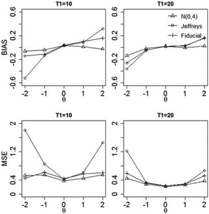
The bias results in Figure 1 show that when T1 only consists of 10 items, using the Jeffreys prior results in larger bias at θ = ±2 than the other two estimation methods; while the three estimation methods lead to similar results at the three medium θ levels, using N(0, $2^2$) results in the lowest bias among the three estimation methods. When the length of T1 increases to 20 items, the bias difference between the three methods becomes smaller at all five θ levels, while using N(0, $2^2$) still results in smaller bias at the two extreme θ levels. The MSE results demonstrate a similar pattern: Using the Jeffreys prior results in much larger MSE at θ = ±2 than the other two estimation methods, especially when T1 is short. Using the fiducial distribution and N(0, $2^2$) leads to quite similar MSE, with the MSE from N(0, $2^2$) being slightly lower.

Figure 1.

Bias and MSE for $\hat{\mathrm{\theta }}$ under three estimation methods.

Note. The two plots in the first row are the results for bias under two lengths of T1. The two plots in the second row are the results for MSE under two lengths of T1. MSE = mean squared error.

Type I Error

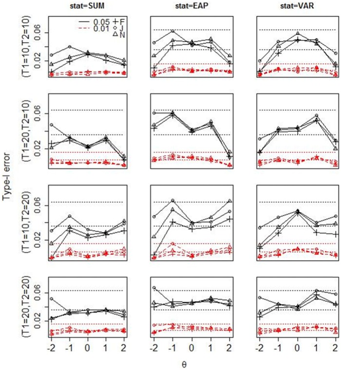
Figure 2 presents the Type I error rates for each test statistic in all conditions. Given the nominal level of 0.05 and 0.01, the 95% normal-approximation confidence intervals for the Type I error out of 1,000 replications are [0.036, 0.063] and [0.004, 0.016], respectively. Results show that using the summed score leads to slightly conservative Type I error rates at most θ levels at all lengths of T1 and T2. Using the EAP and the posterior variance tends to result in conservative Type I error rates at extreme θ levels when T1 or T2 only contains 10 items; as T1 and T2 both consist of 20 items, the Type I error for these two statistics tends to fall in the 95% confidence interval at all θ levels. The conservative Type I error for the summed score at all θ levels is due to the discreteness of its predictive distribution: The summed score only has 11 and 21 possible values when T2 has 10 and 20 items, respectively. Similarly, the conservativeness for EAP or posterior variance also relates to the fact that the predictive distribution concentrates on very few values at the extreme θ levels, especially when T2 is short. Regarding the effect of using different estimation methods, using the Jeffreys prior tends to result in larger Type I error than the other two methods, while using the fiducial distribution tends to result in smaller Type I error. In particular, using the Jeffreys prior could result in slight Type I error inflation for EAP at lower θ levels when T2 contains 20 items, but the inflation is not excessive.

Figure 2.

Type I error for each test statistic under three estimation methods (F = fiducial, J = Jeffreys, N = N(0, $2^2$)) in all simulation conditions.

Note. The first to third columns show the Type I error for the summed score, EAP, and posterior variance, respectively. Each row shows the Type I error under a given length of T1 and T2. The broken lines in each plot show the empirical Type I error at the nominal level of 0.01, and the solid lines show the empirical Type I error at the nominal level of 0.05. The two parallel dotted lines represent the 95% normal-approximation confidence interval for nominal level of 0.01/0.05, respectively. SUM = summed score; EAP = expected a posterior; VAR = posterior variance.

Power

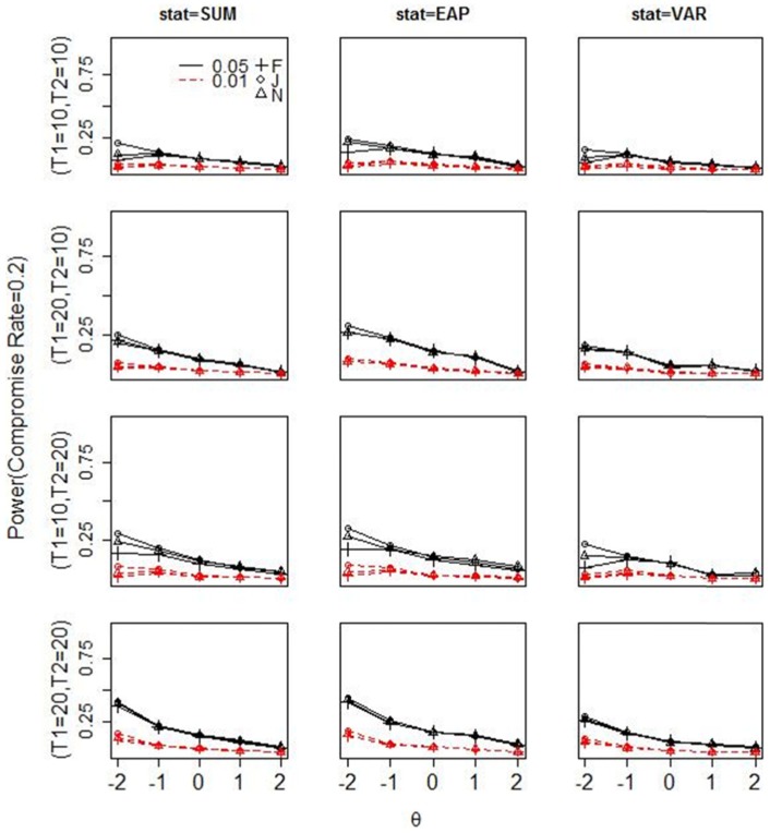
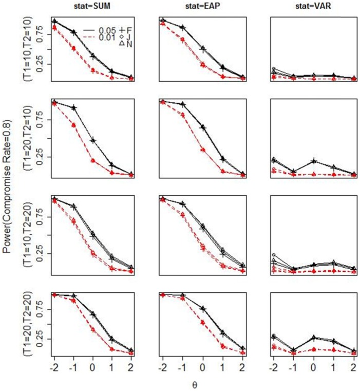
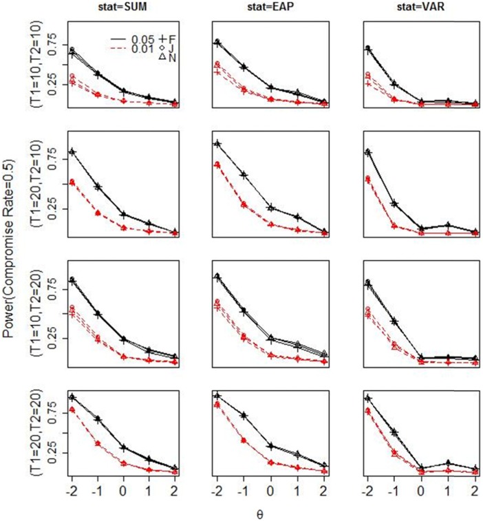
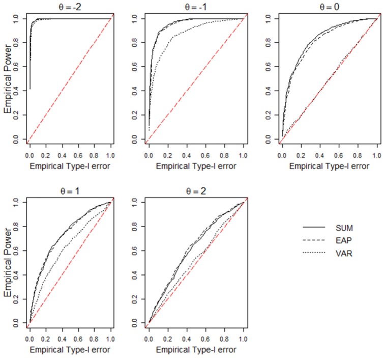
Figures 3 to 5 display the power of each statistic in all simulation conditions. Figure A1 in the appendix shows the receiver operating characteristic (ROC) curve for all three statistics under the condition where T1 and T2 both contain 20 items and the compromise rate is 50%. The power for all three statistics increases as the lengths of T1 or T2 increase. When there is only 20% compromised items in T2, there is no sufficient power for any test statistic: Almost none of them has power above 0.3 when T2 is short; only when T1 and T2 both contain 20 items, the power of the summed score and the EAP reaches around 0.4 at the lowest θ level, given the nominal level of 0.05. As the compromise rate in T2 increases to 0.5, the summed score and EAP have moderate to large power to detect preknowledge among the lowest two θ levels at the nominal level of 0.05, and the posterior variance has similar but slightly lower power than the other two statistics. When 80% items in T2 are compromised, the summed score and EAP have sufficient power to detect preknowledge among $\mathrm{\theta }\le 0$, but the power for posterior variance decreases sharply from that in the 50% compromise condition. The power pattern of the posterior variance at different compromise rates can be explained by the amount of Guttman errors² in a response pattern. When the compromise rate increases from 20% to 50%, the amount of Guttman error increases in a person’s response vector, hence the $\mathrm{\theta }$ posterior distribution becomes more flat and thus the posterior variance becomes larger than expected. However, as the compromise rate increases to 80%, most responses are correct in a person’s response vector, so there are few Guttman errors and the $\mathrm{\theta }$ posterior distribution becomes similar to that estimated from the response vector by a high-proficiency examinee.

Figure 3.

Power for each test statistic under three estimation methods (F = fiducial, J = Jeffreys, N = N(0, $2^2$)) with 20% truly compromised items in T2.

Note. The first to third columns show the power for the summed score, EAP, and posterior variance, respectively. Each row shows the power under a given length of T1 and T2. The broken lines in each plot show the power at the nominal level of 0.01, and the solid lines show the power at the nominal level of 0.05. SUM = summed score; EAP = expected a posterior; VAR = posterior variance.

Figure 5.

Power for each test statistic under three estimation methods with 80% truly compromised items in T2.

Note. SUM = summed score; EAP = expected a posterior; VAR = posterior variance.

Figure 4.

Power for each test statistic under three estimation methods with 50% truly compromised items in T2.

Note. SUM = summed score; EAP = expected a posterior; VAR = posterior variance.

As for the comparison among three statistics, the power difference between EAP and the summed score is at the second decimal place in most conditions. When T2 is short, EAP could have slightly larger power than the summed score at low to medium θ levels, but the power difference is around 0.15 on average. When the compromise rate is high, the posterior variance has much lower power than the other statistics for the reason stated above. At a small or medium compromise rate, the posterior variance demonstrates similar but slightly lower power than the other two statistics, partly because a two-sided test was conducted for it while one-sided tests were conducted for the other statistics. Finally, the three estimation methods lead to very similar power under most conditions. Only when T1 contains 10 items and when the compromise rate is low, the two Bayesian methods exhibit slightly larger power than the fiducial approach at θ = −2.

Real Data Analysis

Data Description

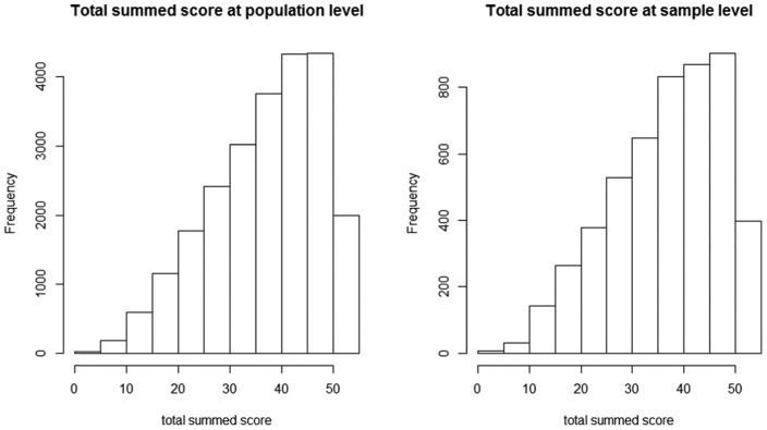
A real data analysis was conducted to demonstrate the practical use of this method. The dataset came from a state assessment measuring students’ math proficiency. The original dataset consisted of 23,583 examinees’ responses to 63 items. As 21 of 63 items were randomly assigned to examinees, there were a lot of missing responses in the file. To simplify the analysis, the 21 randomly assigned items were deleted. The remaining items consisted of 38 dichotomous items and four polytomous items, which were scored 0 to 3. In addition, as the analysis was conducted at the person level, instead of using the entire population, a sample of 5,000 was randomly selected to reduce the computation time. Descriptive analyses on the total test score distribution in the appendix suggest that the selected sample is representative of the population.

Responses to some items were modified to create an artificially compromised dataset. Specifically, 21 items (19 dichotomous items and two polytomous items) were randomly selected from the 42 items as T2. Then, 5% examinees were randomly selected from the examinee sample, and their responses to eight randomly selected items (seven dichotomous items and one polytomous item) in T2 were modified to create the compromised responses. This resulted in a compromise rate around 0.4. An examinee’s response on a compromised dichotomous item was modified to be correct, and one’s score on the compromised polytomous item was increased by 2 points. If the score after manipulation exceeded the maximum possible score, it was set to the maximum.

Data Analysis

As the first step of the analysis, the person fit of responses on the artificially secure section (denoted “T1”) was evaluated for each examinee. As it has been assumed so far that the responses to T1 fit the IRT model, only response vectors not identified as having misfit problems were retained for further analysis. The person fit of responses on T1 was evaluated using the popular person-fit statistic $l_z$ (Drasgow, Levine, & McLaughlin, 1987; Drasgow et al., 1985; Sinharay, 2015). Previous studies have shown that when $\hat{\mathrm{\theta }}$ is used in the $l_z$ calculation, the empirical distribution of $l_z(\hat{\mathrm{\theta }})$ deviates from the asymptotic distribution derived for $l_z(\mathrm{\theta })$. Sinharay (2015) constructed the null distribution of $l_z(\hat{\mathrm{\theta }})$ using the Bayesian posterior predictive checking (PPC; for example, Gelman et al., 2013) approach in a mixed-format test, and found that it led to a larger power than using the asymptotic distribution, and the PPC p value did not have the problem of being conservative in the case with $l_z(\hat{\mathrm{\theta }})$. Therefore, PPC was used to construct the null distribution of $l_z$ in the present study. A nominal level of 0.05 was used to identify misfitting responses.

After removing examinees identified by $l_z$, predictive checking was conducted among the remaining examinees. N(0,2²) was used as the prior distribution as the simulation study showed that the difference between prior configurations was small, and using N(0,2²) led to an easier computation. The summed score and posterior variance were used as the test statistics. The EAP was not used here because the simulation showed that it had very similar power to the summed score when both subsets were long. The three-parameter logistic (3PL) model³ and the graded response model were used as the scoring models for dichotomous and polytomous items, respectively. The detection rates for each test statistic were calculated, respectively, among examinees whose responses have been modified (i.e., modified examinees) and unmodified (i.e., unmodified examinees).

Results

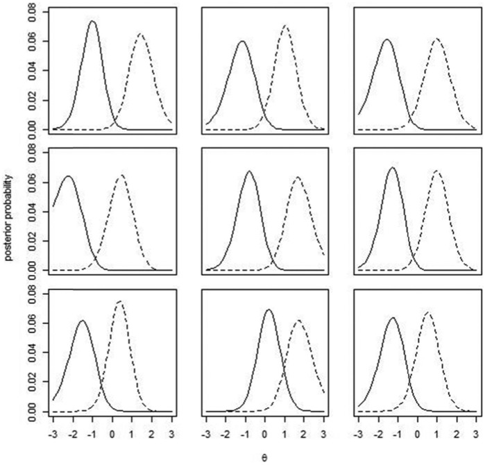
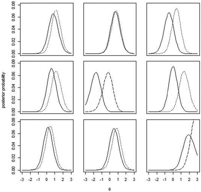
In the first-step analysis of person fit on “T1,” only 1.4% of the sample were detected by $l_z$. Table 1 summarizes the detection rates among the modified examinees and unmodified examinees by each statistic, as well as the average $\hat{\mathrm{\theta }}$ (EAP) increase from T1 to T2 among examinees detected by each statistic. The detection rates among the modified examinees are low, which is likely due to the fact that the test is relatively easy (the average item difficulty is around −0.32), and the total test score distribution is skewed to the left. The simulation results have shown low detection rates among high-proficiency examinees when the compromise rate on T2 is 60%. Among both groups of examinees, the average $\hat{\mathrm{\theta }}$ increase from T1 to T2 is much higher for those detected by the summed score than for those detected by the posterior variance. Figures 6 and 7 display the θ posterior distributions on the two subtests for nine individuals detected by each statistic among modified examinees. For comparison purposes, Figure 7 only shows examinees with an increase in $\hat{\mathrm{\theta }}$ from T1 to T2 but not being detected by the summed score. It is clear that examinees detected by the summed score all show dissimilar posterior distributions between T1 and T2: The $\mathrm{\theta }$ posterior distribution on T2 shifts to the right to a large extent, while using the posterior variance is able to detect examinees with only slight changes between the two posterior distributions. The same pattern is also observed among unmodified examinees.

Table 1.

Detection Rate ($\hat{\mathrm{\theta }}$ Increase From T1-T2) Among Modified and Unmodified Examinees.

	Modified examinees	Unmodified examinees
Summed score	0.18 (1.88)	0.01 (1.72)
Posterior variance	0.09 (.05)	0.10 (−.51)

Note. The number in the parentheses represents the average $\hat{\mathrm{\theta }}$ increase from T1 to T2 among examinees detected by each statistic.

Figure 6.

Examples detected by the summed score among modified examinees.

Note. The solid line represents posterior distribution of θ on T1, and the broken lines represent θ posterior distributions on T2.

Figure 7.

Examples detected by the posterior variance among modified examinees.

Note. The solid line represents posterior distribution of θ on T1, and the broken or dotted lines represent θ posterior distributions on T2. The broken lines indicate that the observed posterior variance is at the right tail of the predictive distribution, and dotted lines indicate that the observed posterior variance is at the left tail.

Discussion and Conclusion

This study proposed a predictive checking method to detect a person’s preknowledge on exposed items by using information from secure items. Considering that the posterior distribution of $\mathrm{\theta }$ estimated from a short secure section might be largely affected by the use of an inappropriately specified prior distribution, the performance of two weakly informative Bayesian priors and the fiducial distribution that does not need to specify a prior distribution was investigated. The $\mathrm{\theta }$ recovery results show that using the Jeffreys prior leads to larger bias and MSE for the point estimate of $\mathrm{\theta }$, but the detection effectiveness among the three methods is quite similar.

Regarding the detection effectiveness under different factors, conservative Type I error is seen among low-ability or high-ability examinees when either section is short, but no Type I error inflation is observed when the fiducial distribution or the N(0, $2^2$) prior is used. As for the detection power, it is hard to detect preknowledge among high-ability examinees in all conditions. Although preknowledge will result in less score inflation for high-ability examinees than for low-ability examinees, it may still affect the decision accuracy if a test’s cut score is set at the higher end of the ability continuum. In addition, not detecting preknowledge among high-ability examinees may fail to resolve test security concerns among a high-proficiency examinee group.

The detection power is largely affected by the proportion of the truly compromised items in T2. Given a large compromise rate, using just 10 items in either section could lead to sufficient power for EAP or the summed score among medium- to low-ability examinees. In comparison, if a large possibly compromised section only contains a small proportion of truly compromised items, the detection power could reduce significantly. Therefore, to maintain the detection power, one can apply predictive checking to items that are most likely to be compromised. Alternatively, one can only include relatively difficult items in the possibly compromised subset, as it is hard to detect preknowledge on easy items by any means. Finally, although the posterior variance exhibits smaller power than the other two statistics in this study, the real data analysis suggests that using it along with the summed score or the EAP can help detect examinees with a relatively small score increase.

There are several limitations of this study. First, this study assumes that the responses to the secure items fit the IRT model well. This is unlikely to happen in practice. For instance, those responses are likely to be affected by some other aberrant response behaviors such as careless responding and test speededness. Future study should evaluate the performance of the predictive checking method when there is misfit in responses to the secure items. In addition, in reality, as it is never certain whether responses to T1 provide an accurate estimate for θ, a reversed predictive checking can be considered: Besides estimating the θ posterior from T1 and conducting checks on T2, one could use T2 to compute the θ posterior and conduct checks on T1. A response vector can be flagged as suspicious if either direction indicates the inconsistency in a person’s response behavior between the two sections. Second, true item parameters were used in conducting person-level analysis, as it was assumed that a large sample would be available for item calibration. The impact of sampling variability of item parameter estimates and model misspecifications on the person-level detection can be investigated in future studies. Third, a simple data generation model was considered to simulate responses in preknowledge conditions, and future studies should explore other models to generate compromised responses. Future studies could also consider incorporating response time model into the predictive checking and incorporate response times as additional information into detection.

Appendix

Figure A1.

Empirical ROC curve for each test statistic at the compromise rate of 0.5.

Note. SUM = summed score; EAP = expected a posterior; VAR = posterior variance; ROC = receiver operating characteristic.

Table A1.

First Four Central Moments of the Total Test Score Distribution in the Population and the Selected Sample.

	M	SD	Skewness	Kurtosis
Population	37.34	10.64	−0.58	2.56
Sample	37.00	10.67	−0.54	2.51

Figure A2.

Total test score distribution at the population (left) and the sample (right) level.

References

- Belov D. I. (2013). Detection of test collusion via Kullback-Leibler divergence. Journal of Educational Measurement, 50, 141-163. [Google Scholar]
- Belov D. I. (2014). Detecting item preknowledge in computerized adaptive testing using information theory and combinatorial optimization. Journal of Computerized Adaptive Testing, 2(3), 37-58. [Google Scholar]
- Brown L. D., Cai T. T., DasGupta A. (2001). Interval estimation for a binomial proportion. Statistical Science, 16, 101-133. [Google Scholar]
- de L. T. J., Deng W. (2008). Improving person-fit assessment by correcting the ability estimate and its reference distribution. Journal of Educational Measurement, 45(2), 159-177. [Google Scholar]
- Drasgow F., Levine M. V., McLaughlin M. E. (1987). Detecting inappropriate test scores with optimal and practical appropriateness indices. Applied Psychological Measurement, 11, 59-79. [Google Scholar]
- Drasgow F., Levine M. V., Williams E. A. (1985). Appropriateness measurement with polychotomous item response models and standardized indices. British Journal of Mathematical and Statistical Psychology, 38, 67-86. [Google Scholar]
- Fisher R. A. (1930). Inverse probability. Proceedings of the Cambridge Philosophical Society, 26, 528-535. [Google Scholar]
- Gelman A., Carlin J. B., Stern H. S., Dunson D. B., Vehtari A., Rubin D. B. (2013). Bayesian data analysis. New York, NY: Chapman & Hall. [Google Scholar]
- Glas C. A. W., Meijer R. R. (2003). A Bayesian approach to person fit analysis in item response theory models. Applied Psychological Measurement, 27(3), 217-233. [Google Scholar]
- Hannig J. (2009). On generalized fiducial inference. Statistica Sinica, 19, 491-544. [Google Scholar]
- Hannig J. (2013). Generalized fiducial inference via discretization. Statistica Sinica, 23, 489-514. [Google Scholar]
- Hannig J., Iyer H., Lai R. C. S., Lee T. C. M. (2016). Generalized fiducial inference: a review and new results. Journal of American Statistical Association, 111, 1346-1361. [Google Scholar]
- Karabatsos G. (2003). Comparing the aberrant response detection performance of thirty-six person-fit statistics. Applied Measurement in Education, 16, 277-298. [Google Scholar]
- Lewis C., Lee Y., von Davier A. A. (2012, May). Test security for multistage tests: A quality control perspective. Paper presented at the Conference on Statistical Detection of Potential Test Fraud, Lawrence, KS. [Google Scholar]
- Li F., Gu L., Manna V. (2004, April). Methods to detect group-level aberrance in state standardized assessment. Paper presented at the National Council on Measurement in Education Meeting, Philadelphia, PA. [Google Scholar]
- Liu Y., Hannig J. (2016). Generalized fiducial inference for binary logistic item response models. Psychometrika, 81, 290-324. [DOI] [PubMed] [Google Scholar]
- McLeod L. D., Lewis C. (1999). Detecting item memorization in the CAT environment. Applied Psychological Measurement, 23, 147-160. [Google Scholar]
- McLeod L. D., Lewis C., Thissen D. (2003). A Bayesian method for the detection of item preknowledge in computerized adaptive testing. Applied Psychological Measurement, 27, 121-137. [Google Scholar]
- Meijer R. R., Sijtsma K. (2001). Methodology review: Evaluating person fit. Applied Psychological Measurement, 25, 107-135. [Google Scholar]
- Metropolis N., Rosenbluth A. W., Rosenbluth M. N., Teller A. H., Teller E. (1953). Equations of state calculations by fast computing machine. Journal of Chemical Physics, 21, 1087-1091. [Google Scholar]
- R Core Team. (2016). R: A language and environment for statistical computing. Vienna, Austria: R Foundation for Statistical Computing. Available; from http://www.R-project.org/ [Google Scholar]
- Rupp A. A. (2013). A systematic review of the methodology for person fit research in item response theory: Lessons about generalizability of inferences from the design of simulation studies. Psychological Test and Assessment Modeling, 55(3), 3-38. [Google Scholar]
- Segall D. (2002). An item response model for characterizing test comprise. Journal of Educational and Behavioral Statistics, 27(2), 163-179. [Google Scholar]
- Sherlock C., Fearnhead P., Roberts G. O. (2010). The random walk Metropolis: Linking theory and practice through a case study. Statistical Science, 25(2), 172-190. [Google Scholar]
- Shu Z., Henson R., Luecht R. (2013). Using deterministic, gated item response theory model to detect test cheating due to item compromise. Psychometrika, 78, 481-497. [DOI] [PubMed] [Google Scholar]
- Sinharay S. (2015). Assessment of person fit for mixed-format tests. Journal of Educational and Behavioral Statistics, 40, 343-365. [Google Scholar]
- Sinharay S. (2017). Detection of item preknowledge using likelihood ratio test and score test. Journal of Educational and Behavioral Statistics, 42, 46-68. [Google Scholar]
- van Krimpen-Stoop E. M. L. A., Meijer R. R. (1999). The null distribution of person-fit statistics for conventional and adaptive tests. Applied Psychological Measurement, 23(4), 327-345. [Google Scholar]