Comparison of Classical Test Theory and Item Response Theory in Individual Change Assessment

Abstract

Clinical psychologists are advised to assess clinical and statistical significance when assessing change in individual patients. Individual change assessment can be conducted using either the methodologies of classical test theory (CTT) or item response theory (IRT). Researchers have been optimistic about the possible advantages of using IRT rather than CTT in change assessment. However, little empirical evidence is available to support the alleged superiority of IRT in the context of individual change assessment. In this study, the authors compared the CTT and IRT methods with respect to their Type I error and detection rates. Preliminary results revealed that IRT is indeed superior to CTT in individual change detection, provided that the tests consist of at least 20 items. For shorter tests, however, CTT is generally better at correctly detecting change in individuals. The results and their implications are discussed.

Individual change assessment plays an important role in clinical practice whereby clinicians are interested in the effectiveness of treatment for individual patients rather than the average improvement of groups of patients as a whole. The assessment of individual change in clinical contexts can be done using either the methodologies of classical test theory (CTT) or item response theory (IRT). CTT approaches are familiar to most clinicians and are therefore widely used, but IRT methods are also gaining popularity.

Several authors have argued that IRT is superior to CTT (e.g., Prieler, 2007; Reise & Haviland, 2005). The most important difference between CTT and IRT is that in CTT, one uses a common estimate of the measurement precision that is assumed to be equal for all individuals irrespective of their attribute levels. In IRT, however, the measurement precision depends on the latent-attribute value. This can result in differences between CTT and IRT with respect to their conclusions about statistical significance of change.

There are other arguments favoring IRT that are worth mentioning. IRT models, including the popular two-parameter logistic and the graded response models (GRMs), take the pattern of item scores into account when inferring latent-attribute scores. This means that the latent-attribute values at pretest and posttest may differ even when the classical pretest and posttest sum scores are equal. As a result, IRT may reveal subtle changes in individuals’ mental health that could go unnoticed if one uses the sum scores from CTT, which ignore the pattern of the item scores. Finally, IRT facilitates adaptive testing, which allows researchers to use different questions at pretest and posttest, provided that the items are all calibrated on the same scale. A major drawback of IRT approaches to change assessment is their reliance on the availability of accurate estimates of the item parameters and model fit, which may be costly and difficult to realize.

Empirical studies comparing CTT and IRT have shown ambiguous results (e.g., Brouwer, 2013; Sébille et al., 2010), suggesting that the CTT approach may be as effective as IRT for assessing individual change. However, so far a systematic head-to-head comparison of the two approaches in the context of individual change assessment has not been done. Given the importance of individual change assessment in clinical settings, the optimism about IRT methods, and the ambiguity of the results of studies comparing CTT and IRT, the authors compared the two methods with respect to individual change assessment. The results of such a comparison can help clinicians and researchers make more informed decisions about scoring tests and assessing change.

This article is organized as follows. First, the authors explained Jacobson and Truax’s (1991; henceforth JT) operationalization of clinically and statistically significant change in the CTT context and extended it to IRT. Then they discussed the design and the results of a simulation study that compares CTT and IRT with respect to Type I error and detection rates in assessing individual change. Finally, they discussed the implications of the results and provided recommendations for researchers and clinicians working in clinical settings.

Operationalization of Individual Change in CTT and IRT

CTT Approach of JT

Reliable change

Let $X$ be the sum score based on the $J$ items in the test with item scores denoted by $X_j(j=1,\dots ,J)$, so that $X=\sum _{j=1}^J{X}_j$. Let $X_{\mathrm{pre}}$ and $X_{\mathrm{post}}$ be the sum scores at pretest and posttest (briefly called pretest and posttest scores), respectively. In what follows, it is assumed that the pretest and posttest scores are obtained on identical tests or questionnaires. Statistical significance of change is assessed by means of the reliable change index (RCI), which JT defined as follows. Let $d=X_{\mathrm{post}}-X_{\mathrm{pre}}$ be the change score for an individual patient. Then, assuming that higher scores reflect worse health conditions, $d<0$ and $d>0$ suggest improvement and deterioration, respectively. Furthermore, let $\mathrm{SE}{\mathrm{M}}_d$ be the standard error of measurement of change score $d$. To assess individual change, the following assumptions are made: (a) equal measurement precision at pretest and posttest, that is, $\mathrm{SE}{\mathrm{M}}_{X_{\mathrm{pre}}}=\mathrm{SE}{\mathrm{M}}_{X_{\mathrm{post}}}=\mathrm{SE}{\mathrm{M}}_X$; (b) uncorrelated measurement errors between pretest and posttest; and (c) measurement invariance, that is, the test is measuring the same latent attribute at pretest and posttest, and the answer categories are interpreted in the same way at pretest and posttest. Using these assumptions, we obtain $\mathrm{SE}{\mathrm{M}}_d=\sqrt{2}\times \mathrm{SE}{\mathrm{M}}_{X_{\mathrm{pre}}}$. JT (1991) defined the RCI as

$$\mathrm{RC}{\mathrm{I}}_{\mathrm{CTT}}=\frac{d}{\mathrm{SE}{\mathrm{M}}_d}.$$

The RCI is assumed to be standard normally distributed in the absence of change. An RCI with an absolute value that exceeds the critical z score corresponding to a desired significance level is considered to represent reliable change. For example, at a two-tailed significance level of $.10$, $\left|\mathrm{RC}{\mathrm{I}}_{\mathrm{CTT}}\right|\ge 1.645$ indicates reliable change, which can either mean improvement or deterioration.

Clinical significance assessment

JT assessed clinical significance of change by evaluating whether a patient’s pretest score moved from the dysfunctional score range to the functional score range at posttest. Let $X_{\mathrm{cut}}$ denote the clinical cutoff separating functional and dysfunctional score ranges. As it is assumed that higher scores reflect worse clinical conditions, clinical significance is inferred if $X_{\mathrm{pre}}>X_{\mathrm{cut}}$ and $X_{\mathrm{post}}<X_{\mathrm{cut}}$. JT defined functional and dysfunctional score ranges based on cutoff scores obtained from either the distribution of the scores in the functional or healthy population, the dysfunctional or clinical population, or both. They proposed to use one of the following cutoffs: (a) the 90th percentile of the score distribution in the functional population, (b) the 10th percentile of the score distribution in the dysfunctional population, or (c) the average of the means of the score distributions in the functional and the dysfunctional populations (see Figure A1 in the online appendix for a graphical explanation of the three cutoffs).

Based on the combination of clinical and statistical significance of change scores and the direction of the observed change, patients can be classified into one of five exhaustive and mutually exclusive change categories (e.g., Bauer, Lambert, & Nielsen, 2004). These are labeled as (a) no change, that is, change is neither statistically nor clinically significant; (b) improvement, that is, change indicates better functioning and is statistically but not clinically significant; (c) recovery, that is, change indicates better functioning which is both statistically and clinically significant; (d) deterioration, that is, change indicates worse functioning which is statistically but not clinically significant; and (e) clinically significant deterioration, that is, change indicates worse functioning which is both statistically and clinically significant. Two remarks are in order. First, for persons to be classified as having deteriorated to a clinically significant degree, change has to be statistically significant and the pretest and posttest scores have to belong to the functional and dysfunctional ranges, respectively. Second, no change means that the observed change is too small to be statistically significant. In practice, nonsignificant change means that more information is needed before reliable conclusions about individual change can be made. Thus, one should not conclude that no change has taken place.

IRT Perspective

Reliable change

The assessment of statistical and clinical significance of individual change in the context of CTT can be readily extended to IRT. Let ${\hat{\mathrm{\theta }}}_{\mathrm{pre}}$ and ${\hat{\mathrm{\theta }}}_{\mathrm{post}}$ be the estimated latent-attribute values at pretest and posttest under the postulated IRT model, respectively. Furthermore, let $\mathrm{SE}({\hat{\mathrm{\theta }}}_{\mathrm{pre}})$ and $\mathrm{SE}({\hat{\mathrm{\theta }}}_{\mathrm{post}})$ be the standard errors for the estimated pretest and posttest scores, respectively. Assuming independent observations at the individual level, the RCI in the context of IRT is defined as

$$\mathrm{RC}{\mathrm{I}}_{\mathrm{IRT}}=\frac{{\hat{\mathrm{\theta }}}_{\mathrm{post}}-{\hat{\mathrm{\theta }}}_{\mathrm{pre}}}{\sqrt{\mathrm{SE}{\left({\hat{\mathrm{\theta }}}_{\mathrm{pre}}\right)}^2+\mathrm{SE}{\left({\hat{\mathrm{\theta }}}_{\mathrm{post}}\right)}^2}}.$$

Equation 2 requires estimates of the latent-attribute values, ${\hat{\mathrm{\theta }}}_{\mathrm{pre}}$ and ${\hat{\mathrm{\theta }}}_{\mathrm{post}}$. Research showed that weighted maximum likelihood (WML) produces estimates having the smallest bias and the greatest precision (e.g., Jabrayilov, 2016; Wang & Wang, 2001). Standard errors are obtained by means of the information function (e.g., Reise & Haviland, 2005). IRT-based individual change assessment requires the availability of accurate estimates of all item parameters, for example, by means of multiple-group IRT models when data are obtained from both general and clinical populations. Henceforth, we assume that this requirement is met and use the true item parameters for estimating the person parameters. In addition, unlike CTT, IRT methods do not require pretest and posttest measurements to be based on the same items as long as all items are calibrated on the same scale. However, to fairly compare CTT and IRT, the same items were used at pretest and posttest.

Clinical significance assessment

In an IRT context, clinical significance can be assessed by examining whether the latent attribute value has passed a clinical cutoff. The crucial difference between CTT and IRT is that in CTT the cutoffs are based on the distribution of the sum scores $X$, whereas in IRT they are based on the $\mathrm{\theta }$ distribution. For example, in the IRT context, JTs cutoff ($a$) would be the 90th percentile of the $\mathrm{\theta }$ distribution in the functional population.

Comparing Measurement Precision in CTT and IRT

One of the main arguments for favoring IRT methods is that they allow using the local precision of the estimated scores, $\mathrm{SE}(\hat{\mathrm{\theta }})$, to test change for significance, whereas in CTT, one common population-level SEM is used for all persons. Because the population-level SEM used in CTT is the average of the individual SEMs (Mellenbergh, 2011) which vary across individuals, using a SEM which is too large results in underestimating measurement precision of the scores in the tails of the distribution, whereas using a SEM which is too small results in overestimating measurement precision of the scores in the middle of the distribution (e.g., Mollenkopf, 1949; see Figure 1, upper graph, for population-level constant SEM and the empirical standard error for observed scores). Therefore, using SEM may bias decisions based on the RCI.

Figure 1.

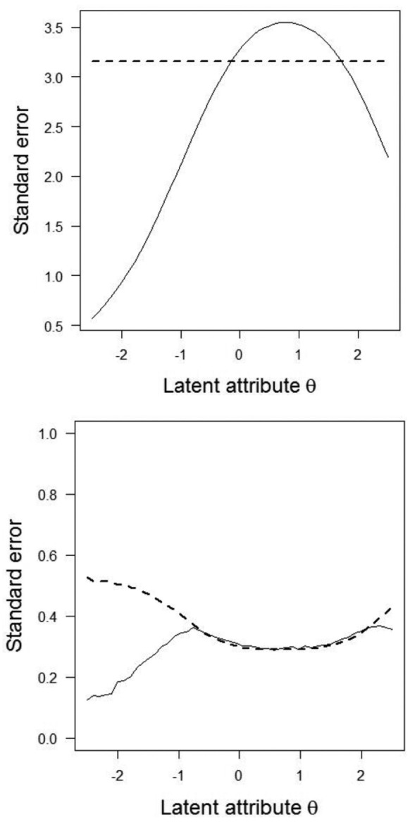
Comparison of standard errors of estimated person scores in CTT (upper graph) and IRT (lower graph).

Note. Upper panel: Solid line represents empirical standard error of X as a function of latent-attribute $\mathrm{\theta }$, dashed line represents SEM. Lower panel: Solid line represents empirical standard error of WML estimates $\hat{\mathrm{\theta }}$ as a function of $\mathrm{\theta }$, dashed line represents the asymptotic standard error based on square root of the inverse of Fisher information function. CTT = classical test theory; IRT = item response theory; SEM = standard error of measurement; WML = weighted maximum likelihood.

The standard errors in Equation 2 are usually obtained using the Fisher information function evaluated at $\hat{\mathrm{\theta }}$, but are only accurate if the number of items is sufficiently large, say, more than $20$ (Magis, 2014). Clinical practice shows a tendency for using short scales to minimize the burden on patients (Kruyen, Emons, & Sijtsma, 2013). When $\mathrm{\theta }$ is estimated from a limited number of discrete item scores, asymptotic results no longer apply and the corresponding estimated standard errors may be inaccurate (Jabrayilov, 2016). To illustrate this point, suppose that one repeatedly tests the same patient having an extremely high $\mathrm{\theta }$ value under identical conditions. Hypothetically, one expects the same pattern of $J$ maximum item scores at each replication; hence, the patient obtains the same $\hat{\mathrm{\theta }}$ each time, and the empirical standard error is small. For high $\mathrm{\theta }$ values, however, test information is low, and thus, the asymptotic standard error is large. Hence, for extreme $\mathrm{\theta }$ values, IRT methods tend to overestimate the empirical standard errors when scales are short. For a 10-item test with varying difficulties, Figure 1 (lower graph) shows the relationship between estimated asymptotic standard errors and empirical standard errors.

Given the differences between CTT and IRT with respect to change assessment, depending on which method one uses, we expect that different conclusions may be drawn about change in individual patients. Because of the high expectations regarding IRT as a refinement and an improvement relative to CTT, we were particularly interested in finding out whether, compared with CTT, IRT produces more precise Type I error and higher detection rates of clinically significant change. We used a simulation study to this end.

Method

Data Generation

Person characteristics

In both the healthy and clinical populations, we assumed normal distributions for latent-attribute $\mathrm{\theta }$ with variance of 1 and means of 0 and 0.5, respectively. Because within-population variances equaled 1, using Cohen’s $d$ (Cohen, 1988) the difference between the means corresponded to a medium effect size between the healthy and clinical populations. Standard normality of $\mathrm{\theta }$ in the healthy population was an arbitrary choice that serves to identify the $\mathrm{\theta }$ scale (e.g., Embretson & Reise, 2000).

Test and item characteristics

Pretest and posttest item scores were modeled using the GRM (Embretson & Reise, 2000; Samejima, 1970). Invariant item parameters were assumed between pretest and posttest (i.e., measurement invariance). Let $M+1$ denote the number of ordered item scores for an item, and let item score $X_j$ have realizations $x_j(x_j=0,\dots ,M)$. The GRM models the probabilities of obtaining a particular item score $x_j$ or a higher score by means of $M$ cumulative response functions, each defined by a two-parameter logistic function:

$$P_{j{x}_j}^{*}\left(\theta \right)=P(X_j\ge x_j|\mathrm{\theta })=\frac{\exp \left[a_j(\mathrm{\theta }-b_{j{x}_j})\right]}{1+\exp \left[a_j(\mathrm{\theta }-b_{j{x}_j})\right]},x_j=1,\dots ,M.$$

By definition, $P_{j0}^{*}(\mathrm{\theta })=1$ and $P_{j,M+1}^{*}(\mathrm{\theta })=0$. The probabilities of obtaining score $x_j$ can be obtained by subtracting the cumulative response probabilities, for $X_j\ge x_j$ and $X_j\ge x_j+1$ (Embretson & Reise, 2000). In Equation 3, $a$ ($a_j>0$) represents the slope parameter for item $j$ indicating how well the item discriminates between respondents with different levels of $\mathrm{\theta }$, and $b_{j{x}_j}$ is the threshold parameter indicating the value of $\mathrm{\theta }$ where $P_{j{x}_j}^{*}(\mathrm{\theta })=.50$ and the location on the $\mathrm{\theta }$ scale where the response function has its maximum slope discriminating different $\theta \mathrm{s}$ best. Hence, each item was modeled by $M$ threshold parameters $b_{j{x}_j}(x_j=1,\dots ,M)$, which had a fixed ordering $b_{j1}\le \cdots \le b_{\mathrm{jM}}$. In this study, items were scored from 0 to 4, higher scores indicating worse health conditions. Hence, each item had four $b$ parameters ($M=4$).

Item parameters were chosen in two conditions. To guarantee a fair comparison between CTT and IRT, we chose the item parameters such that adequate psychometric properties were obtained both in terms of CTT and IRT. In the first condition, the item parameters were defined representing tests for narrow attributes such as depression and anxiety (Reise & Waller, 2009). We sampled discrimination parameters ($a$) from $U(1.5;2.5)$. Following Emons, Sijtsma, and Meijer (2007), the threshold $b\mathrm{s}$ were sampled as follows. Let ${\overline{b}}_j$ represent the average threshold of item $j$. For each item, we first sampled ${\overline{b}}_j$ from $U(0;1.25)$ and then the four individual $b\mathrm{s}$ were obtained as follows: $b_{j1}={\overline{b}}_j-1$, $b_{j2}={\overline{b}}_j-0.5$, $b_{j3}={\overline{b}}_j+0.5$, and $b_{j4}={\overline{b}}_j+1$; hence, item mean variation was small. The name of homogeneous item-difficulty condition suggested that the mean item-level difficulties were concentrated on a limited range of the θ scale.

The second condition represented the characteristics of tests that typically measure potentially broader attributes such as personality traits and quality of life. Reise and Waller (2009) argued that the item difficulties in broad-attribute tests are usually spread across the entire latent-attribute scale and on average have somewhat lower discrimination than items in narrow-attribute tests. Therefore, compared with the previous condition, we sampled the discrimination parameters ($a$s) and the mean thresholds ${\overline{b}}_j\mathrm{s}$ from a wider interval, the $a\mathrm{s}$ from $U(1;2.5)$ and ${\overline{b}}_j\mathrm{s}$ from $U(-1.5;2.5)$. The $b\mathrm{s}$ were selected such that the expected mean item scores also varied from low to high. This resulted in $b\mathrm{s}$ that were located closer to the ${\overline{b}}_j\mathrm{s}$ than in the homogeneous item-difficulty condition. The $b\mathrm{s}$ equaled $b_{j1}={\overline{b}}_j-0.5$, $b_{j2}={\overline{b}}_j-0.2$, $b_{j3}={\overline{b}}_j+0.2$, and $b_{j4}={\overline{b}}_j+0.5$. The second condition’s name is heterogeneous item-difficulty condition, expressing spread of item-level difficulties along the entire latent-attribute scale. The healthy and clinical populations had mean coefficient alpha at least equal to $.7$ and item-rest score correlations which exceeded .$3$. In the homogeneous item-difficulty condition, mean item scores ranged from $0.81$ to $2.52$ (on a scale running from 0 to 4) and in the heterogeneous item-difficulty condition from $0.11$ to $3.75$. Hence, the simulation setup generated data that are realistic both in terms of CTT and IRT characteristics.

Determination of Cutoffs for Assessing Clinical Significance

Clinical cutoffs in IRT

Following JT (1991), the authors defined three different cutoffs: that is, for cutoff $(a)$, they placed the cutoff at the 90th percentile of the $\theta$ distribution in the healthy population (i.e., ${\mathrm{\theta }}_{\mathrm{cut}}=1.28$); for cutoff $(b)$ at the 10th percentile of the $\mathrm{\theta }$ distribution in the clinical population (i.e., ${\mathrm{\theta }}_{\mathrm{cut}}=-0.78$); and for cutoff $(c)$ they chose the average of the two population means of $\mathrm{\theta }$ (i.e., ${\mathrm{\theta }}_{\mathrm{cut}}=0.25$).

Clinical cutoffs in CTT

Because in CTT the clinical cutoffs are derived from the sum-score ($X$) distribution, which depends on both the item characteristics and the latent-attribute ($\mathrm{\theta }$) distribution, the authors first obtained the population-level X distributions given the IRT item and person parameters and then they determined the JT cutoffs $(a)$, $(b)$, and $(c)$ from these distributions. In particular, let the item parameters of the GRM be collected in matrix $\mathrm{\xi }$ of order $J$ by 5 (one slope and four threshold parameters). Furthermore, for the healthy (indexed by $H$) and clinical populations (indexed by $C$), let $f_H(X|\mathrm{\xi })$ and $f_c(X|\mathrm{\xi })$ be the discrete marginal distributions of $X$ given item parameters $\mathrm{\xi }$. To obtain the marginal sum-score distributions, in each population the $\mathrm{\theta }$ distribution was approximated using $500$ quadrature points. For cutoff $(a)$, they selected the value of $X$ that was closest to the 90th percentile of $f_H(X|\mathrm{\xi })$; for cutoff $(b)$, they selected the X value closest to the 10th percentile of $f_C(X|\mathrm{\xi })$; and for cutoff $(c)$, they used the average of the two means of the two marginal $X$ distributions. See the online supplement for details.

Simulation Design

The following four design factors were used:

1. Change-assessment method: CTT and IRT.

2. Test length: To mimic scales used in practical clinical contexts, test length was either $5$, $10$, or $20$ items. Examples of tests with similar test lengths are Outcome Questionnaire (OQ-45; Lambert et al., 1996; Social Role subscale = nine items; Interpersonal Relations subscale = 11 items; and Symptom Distress subscale = 25 items), Montgomery–Asberg Depression Rating Scale (Montgomery & Asberg, 1979; 10 items), and Beck Depression Inventory (Beck, Ward, Mendelson, Mock, & Erbaugh, 1961; 21 items).

3. Magnitude of true change: True change had four levels: $\mathrm{\delta }=0$ (no change), $\mathrm{\delta }=-0.5$ (small change), $\mathrm{\delta }=-1$ (medium change), and $\mathrm{\delta }=-1.5$ (large change). Because clinical treatment focuses on improvement, we concentrated on change reflecting improvement (i.e., $\mathrm{\delta }\le 0$). Also, because in this simulation study the direction of the change does not have an intrinsic meaning, we considered the results also be representative of detecting deterioration.

4. Item characteristics: Homogeneous and heterogeneous mean item difficulties.

The design was a fully crossed factorial, with $2$ (CTT, IRT) × 3 (test length) × 4 (true change) × 2 (item characteristics) = 48 cells. In each cell, change scores were simulated as follows. We chose $500$ equally spaced pretest $\mathrm{\theta }$ values (i.e., ${\mathrm{\theta }}_{\mathrm{pre}}$) between $-2.5$ and $3.5$. For each ${\mathrm{\theta }}_{\mathrm{pre}}$ value, we simulated 5,000 pairs of item-score vectors, one for the pretest and one for the posttest. The $\mathrm{\theta }$ value used for generating posttest data depended on the pretest value ${\mathrm{\theta }}_{\mathrm{pre}}$ and true change $\mathrm{\delta }$; that is, ${\mathrm{\theta }}_{\mathrm{post}}={\mathrm{\theta }}_{\mathrm{pre}}+\mathrm{\delta }$. For each pair of item-score vectors, we estimated pre- and posttest latent-attribute values ($\hat{\mathrm{\theta }}$) using WML estimation and computed the observed change and the RCI_IRT (Equation 2). For each pair, we also computed the sum scores at pretest and posttest, the observed change $(d)$, and the RCI_CTT (Equation 1) using the population-based value of the SEM in the clinical population (see online supplement, Table A1, for details). This resulted in $5,000$ replications of CTT and IRT-based individual change assessment at each value of ${\mathrm{\theta }}_{\mathrm{pre}}$. The complete design was replicated $100$ times, each time using newly sampled ${\mathrm{\alpha }}_j$ and ${\overline{b}}_j$ parameters.

Dependent Variable

The dependent variable was the individual classification with respect to individual change in the following three exhaustive and mutually exclusive categories of individual change: (a) no change, (b) improvement, and (c) recovery. We used a $.10$ significance level for testing statistical significance.

To present the results, we made a distinction between classifications under the zero true change condition ($\mathrm{\delta }=0$) and the other conditions (i.e., $\mathrm{\delta }<0$). In the zero true change condition, patients whose observed scores showed recovery or improvement did not really change, and hence constituted Type I errors. Thus, the percentage of classifications in either the recovery or improvement condition (i.e., patients showing reliable change irrespective of whether the change is clinically significant) was reported as Type I error rates. For all other conditions ($\mathrm{\delta }<0$), we reported population-level percentages of correct classifications into either improvement or recovery categories. The population-level percentage is a weighted average of the percentages at all $\mathrm{\theta }$ levels, where the weights are based on the $\mathrm{\theta }$ distributions (see the online appendix). Overall percentages were referred to as detection rates.

For the simulations, the authors developed dedicated software in C++. All other computations were done in R (R Development Core Team, 2014). Source code for C++ and R are available upon request from the corresponding author.

Results

Zero Change

In general, Type I errors were close to the nominal level, but for CTT they were slightly closer to the nominal $\mathrm{\alpha }=.10$ than those for IRT (results not tabulated). In both the homogeneous and heterogeneous item-difficulty conditions, CTT had equal Type I error rates irrespective of test length. In contrast, for IRT, increasing the test length pulled the Type I error rates closer to the nominal Type I error.

Figure 2 shows the Type I error rates as a function of $\mathrm{\theta }$. For CTT, for homogeneous tests, the Type I error rates were above nominal level $\mathrm{\alpha }$ in the middle range of the clinical population distribution and below nominal level $\mathrm{\alpha }$ at the tails. However, for heterogeneous tests, Type I error rates were at or below nominal $\mathrm{\alpha }$. For IRT, both in the homogeneous and heterogeneous item-difficulty conditions, the Type I error rates were at or below the nominal level across the entire scale range, with larger differences at the extremes. These results are consistent with standard errors being underestimated by the group-based SEM from CTT in the middle range of the distribution and overestimated in its tails. Moreover, the asymptotically derived standard errors in IRT tend to overestimate the SE, particularly in the tails of the $\mathrm{\theta }$ scale. This effect diminishes as the number of items increases. That is why increasing test length in IRT pushed the Type I error rates closer to the nominal Type I error rate across a wider range of the $\mathrm{\theta }$ scale.

Figure 2.

Type I error rates in the homogeneous (upper panel) and heterogeneous (lower panel) item-difficulty conditions.

Note. CTT = classical test theory; IRT = item response theory.

Detecting Improvement

Table 1 shows the mean percentage of improved persons (i.e., $\mathrm{\delta }<0$, but true change is not clinically significant) that both CTT and IRT detected. In general, differences between CTT and IRT were the largest for short tests ($J=5$), large change ($\mathrm{\delta }=-1.5$), and homogeneous item difficulties, where the highest mean difference was $18$% in favor of CTT. Comparable detection rates were found for the three cutoff points. CTT had higher detection rates than IRT for five-item tests in all conditions and 10-item tests in the majority of the conditions; mean differences ranged from 1% to 18%. For the 20-item tests, IRT had higher detection rates than CTT in most conditions; mean differences ranged from 1% to 10%. For heterogeneous item-difficulty tests, on average CTT had higher detection rates for five-item tests (mean difference ranged from 2% to 12%) and IRT for 20-item tests (mean difference ranged from 1% to 9%). Results were ambiguous for the 10-item condition. Increasing test length and the true change increased detection rates both for CTT and IRT.

Table 1.

Population-Level Classification Rates (Percentages Averaged Across 100 Replications) for Detecting Improvement in the Clinical Population, for Varying Test Length, Test Model, Item-Location Spread, and Three Cutoff Models.

Cutoff	Homogeneous item difficulty						Heterogeneous item difficulty
	5		10		2 0		5		10		20
	CTT	IRT	CTT	IRT	CTT	IRT	CTT	IRT	CTT	IRT	CTT	IRT
Small change $(\mathrm{\delta }=-0.5)$
a	13	8	24	22	40	41	7	4	13	13	22	26
b	18	13	28	25	44	43	11	6	15	15	24	27
c	8	6	18	18	34	37	4	3	9	10	18	23
Medium change $(\mathrm{\delta }=-1.0)$
a	29	20	54	51	75	78	17	10	33	35	56	64
b	41	32	63	60	80	79	23	15	37	37	58	64
c	18	11	40	39	64	69	9	6	23	24	45	55
Large change $(\mathrm{\delta }=-1.5)$
a	45	27	69	58	82	77	30	17	54	52	77	80
b	61	51	75	71	77	76	37	26	56	55	74	75
c	24	12	49	36	68	61	15	8	36	32	62	66

Note. Reliable change was tested at a nominal significance level of .10. Standard errors for differences between percentages ranged from 0.1% to 0.8%. CTT = classical test theory; IRT = item response theory.

Detecting Recovery

With respect to detecting recovery (i.e., clinical and statistical change), the largest differences between CTT and IRT with respect to mean detection rate were approximately equal to 12% (Table 2). For five-item tests, CTT had higher detection recovery than IRT across all levels of true change; differences varied between 2% and 13%. For 20-item tests, for the majority of the conditions, IRT had higher detection rates than CTT; mean differences ranged from 2% to 13%. Results were consistent across homogeneous and heterogeneous item-difficulty tests and the three cutoff points (($a$), ($b$), and ($c$)). For 10-item tests, results were ambiguous. In some conditions, CTT produced better detection rates than IRT, and vice versa in other conditions. Again, increasing test length and true change increased detection rates both for CTT and IRT.

Table 2.

Population-Level Classification Rates (Percentages Averaged Across 100 Replications) for Detecting Recovery in the Clinical Population, for Varying Test Length, Test Model, Item-Location Spread, and Three Cutoff Models.

Cutoff	Homogeneous tests						Heterogeneous tests
	5		10		20		5		10		20
	CTT	IRT	CTT	IRT	CTT	IRT	CTT	IRT	CTT	IRT	CTT	IRT
Small change $(\mathrm{\delta }=-0.5)$
a	22	17	33	29	49	47	13	9	18	18	28	31
b	6	3	12	15	23	35	8	4	12	14	19	26
c	23	18	34	31	49	48	14	10	19	20	28	31
Medium change $(\mathrm{\delta }=-1.0)$
a	47	42	68	67	82	82	27	21	41	44	63	68
b	16	9	34	38	59	70	16	11	29	33	47	59
c	48	40	68	68	81	83	29	22	44	47	63	69
Large change $(\mathrm{\delta }=-1.5)$
a	69	65	83	83	89	89	44	36	64	67	80	83
b	28	16	55	50	78	76	26	18	47	51	69	77
c	68	57	82	82	87	90	47	35	67	70	81	85

Note. Reliable change was tested at a nominal significance level of .10. Standard errors for differences between percentages ranged from 0% to 0.8%. CTT = classical test theory; IRT = item response theory.

Discussion

A thorough methodological comparison of CTT and IRT with respect to individual change assessment was absent thus far. The authors conclude that IRT is superior to CTT, provided that tests contain, say, at least 20 items, but in general the differences between the two methods are small. For shorter tests, results are ambiguous and using CTT seems to be a good choice. Instead of recommending the exclusive use of IRT for individual change assessment (e.g., Prieler, 2007), they safely conclude that CTT and IRT each have their own advantages and disadvantages in different testing situations.

To minimize the burden on patients, shorter tests containing, say, approximately five items may be preferred in clinical settings (e.g., Kruyen et al., 2014). Here, CTT seems to better detect change than IRT, but one may notice that detection rates in the change conditions (i.e., $\mathrm{\delta }<0$) should be interpreted taking into account the empirical Type I error rates in the no change conditions (i.e., $\mathrm{\delta }=0$). For short tests, for homogeneous item-difficulty tests, the (unknown) empirical Type I error rates generally were higher for CTT than for IRT, and in the middle of the $\mathrm{\theta }$ scale Type I error rates were just above the nominal $\mathrm{\alpha }$ level. Thus, for short tests IRT suggests individual change less frequently than CTT. This may partly explain why CTT more readily identifies improvement or recovery. Moreover, because psychotherapies are meant to bring about recovery or at least improvement, the occurrence of zero true change in patients is rare in practice, thus causing Type II errors (i.e., concluding a patient did not change when in fact he or she did) to be more of a concern than Type I errors.

In general, because for short tests both in CTT and IRT the detection rates were generally low (below 50%) when true change was small ($\mathrm{\delta }=-0.5$) or medium ($\mathrm{\delta }=-1$), the authors did not recommend using short tests if such small changes are deemed clinically important. For large true change, detection rates were higher but a true change of this magnitude may be rare in practice. Future research may focus on empirical applications of IRT-based change assessment to gain more insight in the typical effect sizes. To summarize, they recommend using (a) tests containing at least 20 items and (b) IRT for scoring the tests. However, if the time and resources for administering longer tests are unavailable, they recommend using CTT which has more power when using short tests for detecting change in individuals. Another alternative based on IRT methodology is to use adaptive testing (Finkelman, Weiss, & Gyenam, 2010). In adaptive testing, the questionnaire is tailored to the current level of functioning whereby extreme scores due to floor or ceiling effects can be avoided.

IRT-based individual change assessment is contingent on the fit of the model to the data. The greater the misfit between IRT model and data, the less accurate individual change assessment is. Empirical evidence (Meijer & Baneke, 2004; Waller & Reise, 2010) suggests that traditional parametric models such as the GRM may be too restrictive to accurately describe clinical questionnaire data. Little is known about the robustness of individual change assessment against model violations. CTT methods may be a safer choice when IRT model fit is questionable or inadequately demonstrated. Moreover, IRT methods require substantial sample sizes to obtain accurate parameter estimates, rendering CTT a justifiable alternative when samples are smaller. Second, most clinicians are familiar with the basic CTT concepts such as reliability and SEM, but they lack sufficient knowledge of IRT. As individual change assessment also serves as a way to communicate between the clinician and the patient, it is important that the measurements used have a clear meaning to all parties involved.

The RCI, whether defined under CTT or IRT, assumes uncorrelated measurement errors within individuals. However, when errors are positively correlated, RCI values are too low. Such conservative RCI estimates are not necessarily problematic because researchers maintain control over the Type I error rates while power remains sufficient to detect clinically relevant change. Furthermore, for low-stakes decisions (e.g., monitoring individuals throughout treatment), loss of power can be partly compensated by using a higher $\mathrm{\alpha }$ level (e.g., .10 instead of .05). When measurement errors are negatively correlated, RCIs are overestimated. Such liberal RCIs are problematic because they may overestimate treatment effects. Hypotheses about correlation of measurement errors across time can be tested using covariance structure analysis (e.g., Singer & Wilett, 2003). In case of anticipated negatively correlated errors, one should avoid using the RCI. More importantly, when measurement errors correlate across time, it is questionable whether individual change scores can be interpreted meaningfully at all because they may suggest undesirable idiosyncratic responding.

The authors used clinical cutoffs based on a fixed standardized difference of 0.5 between the functional and the dysfunctional populations. This resulted in cutoffs that were located either at the lower end, the middle, or the higher end of the latent-attribute scale. Consequently, the three cutoffs in this study represent clinical decisions at very different ranges of the latent-attribute scale rendering the results generalizable to many practical situations. In practice, populations may be further apart resulting in an increase of the standardized mean difference (Cohen’s d), but then the JT cutoffs (a) and (b) are pulled toward cutoff (c).

For detecting clinical change, the authors used the JT’s approach, which uses clinical cutoffs representing different levels of functioning. The use of clinical cutoffs for interpreting the clinical meaning of outcome measures is common. However, JT’s method ignores the clinical relevance of change within either the clinical or functional range. Moreover, the cutoffs are based on sample data and thus are susceptible to sampling error. Another popular approach for operationalizing clinical significance is to define what constitutes minimum clinically important differences (MCIDs; for example, Copay, Subach, Glassman, Polly, & Schuler, 2007). Observed change that exceeds this predetermined value is considered clinically relevant. A common choice for the MCID is a half standard deviation of pretest scores. Research (e.g., Norman, Sloan, & Wyrwich, 2003) showed that change that is reliable is also clinically meaningful using an MCID based on the half standard deviation rule. Hence, results for detecting reliable change when true change is 0.5 in general also apply to detecting minimally clinical significant change of a half standard deviation.

References

- Bauer S., Lambert M., Nielsen S. L. (2004). Clinical significance methods: A comparison of statistical techniques. Journal of Personality Assessment, 82, 60-70. [DOI] [PubMed] [Google Scholar]
- Beck A. T., Ward C. H., Mendelson M., Mock J., Erbaugh J. (1961). An inventory for measuring depression. Archives of General Psychiatry, 4, 561-571. [DOI] [PubMed] [Google Scholar]
- Brouwer D., Meijer R. R., Zevalkink J. (2013). Measuring individual significant change on the Beck Depression Inventory-II through IRT-based statistics. Psychotherapy Research, 23, 489-501. [DOI] [PubMed] [Google Scholar]
- Cohen J. (1988). Statistical power analysis for the behavioral sciences. Hillsdale, NJ: Lawrence Erlbaum. [Google Scholar]
- Copay A. G., Subach B. R., Glassman S. D., Polly D. W., Schuler T. C. (2007). Understanding the minimum clinically important difference: A review of concepts and methods. The Spine Journal, 7, 541-546. [DOI] [PubMed] [Google Scholar]
- Embretson S. E., Reise S. P. (2000). Item response theory for psychologists. Mahwah, NJ: Lawrence Erlbaum. [Google Scholar]
- Emons W. H. M., Sijtsma K., Meijer R. R. (2007). On the consistency of individual classification using short scales. Psychological Methods, 12, 105-120. [DOI] [PubMed] [Google Scholar]
- Finkelman M. D., Weiss D. J., Gyenam K.-K. (2010). Item selection and hypothesis testing for the adaptive measurement of change. Applied Psychological Measurement, 34, 238-254. [Google Scholar]
- Jabrayilov R. (2016). Improving individual change assessment in clinical, medical, health psychology (Unpublished doctoral dissertation). Tilburg University, The Netherlands. [Google Scholar]
- Jacobson N. S., Truax P. (1991). Clinical significance: A statistical approach to defining meaningful change in psychotherapy research. Journal of Consulting and Clinical Psychology, 59, 12-19. [DOI] [PubMed] [Google Scholar]
- Kruyen P. M., Emons W. H. M., Sijtsma K. (2013). On the shortcomings of shortened tests: A literature review. International Journal of Testing, 13, 223-248. [Google Scholar]
- Kruyen P. M., Emons W. H. M., Sijtsma K. (2014). Assessing individual change using short tests and questionnaires. Applied Psychological Measurement, 38, 201-216. [Google Scholar]
- Lambert M. J., Hansen N. B., Umphress V., Lunnen K., Okiishi J., Burlingame G., Reisinger C. W. (1996). Administration and scoring manual for the Outcome Questionnaire (OQ45.2). Wilmington, DE: American Professional Credentialing Services. [Google Scholar]
- Magis D. (2014). Accuracy of asymptotic standard errors of the maximum and weighted likelihood estimators of proficiency levels with short tests. Applied Psychological Measurement, 38, 105-121. [Google Scholar]
- Meijer R., Baneke J. J. (2004). Analyzing psychopathology items: A case for nonparametric item response theory modeling. Psychological Methods, 9, 354-368. [DOI] [PubMed] [Google Scholar]
- Mellenbergh G. J. (2011). A conceptual introduction to psychometrics. Den Haag, The Netherlands: Eleven International. [Google Scholar]
- Mollenkopf W. G. (1949). Variation of the standard error of measurement. Psychometrika, 14, 189-229. [DOI] [PubMed] [Google Scholar]
- Montgomery S. A., Asberg M. (1979). A new depression scale designed to be sensitive to change. British Journal of Psychiatry, 134, 382-389. [DOI] [PubMed] [Google Scholar]
- Norman G. R., Sloan J. A., Wyrwich K. W. (2003). Interpretation of changes in health-related quality of life: The remarkable universality of half a standard deviation. Medical Care, 41, 582-592. [DOI] [PubMed] [Google Scholar]
- Prieler J. A. (2007). So wrong for so long: Changing our approach to change. The Psychologist, 20, 730-732. [Google Scholar]
- R Development Core Team. (2014). R: A language and environment for statistical computing. Vienna, Austria: R Foundation for Statistical Computing; Available from http://www.R-project.org [Google Scholar]
- Reise S. P., Haviland M. G. (2005). Item response theory and the measurement of clinical change. Journal of Personality Assessment, 84, 228-238. [DOI] [PubMed] [Google Scholar]
- Reise S. P., Waller N. G. (2009). Item response theory and clinical measurement. Annual Review of Clinical Psychology, 5, 27-48. [DOI] [PubMed] [Google Scholar]
- Samejima F. (1969). Estimation of latent ability using a response pattern of graded scores (Psychometric Monograph No. 17). Richmond, VA: Psychometric Society; Retrieved from http://www.psychometrika.org/journal/online/MN17.pdf [Google Scholar]
- Sébille V., Hardouin J.-B., Le Neel T., Kubis G., Boyer F., Guillemin F., Falissard B. (2010). Methodological issues regarding power of classical test theory and IRT-based approaches for the comparison of patient-reported outcome measures—A simulation study. Medical Research Methods, 10, 1-10. [DOI] [PMC free article] [PubMed] [Google Scholar]
- Singer J. D., Willett J. B. (2003). Applied longitudinal data analysis. New York, NY: Oxford University Press. [Google Scholar]
- Waller N. G., Reise S. P. (2010). Measuring psychopathology with non-standard item response theory models: Fitting the four-parameter model to the Minnesota Multiphasic Personality Inventory. In Embretson S. E. (Ed.), Measuring psychological constructs: Advances in model-based approaches (pp. 147-173). Washington, DC: American Psychological Association. [Google Scholar]
- Wang S., Wang T. (2001). Precision of Warm’s weighted likelihood estimates for a polytomous model in computerized adaptive testing. Applied Psychological Measurement, 25, 317-331. [Google Scholar]
Associated Data
This section collects any data citations, data availability statements, or supplementary materials included in this article.