An analysis of neural receptive field plasticity by point process adaptive filtering

Abstract

Neural receptive fields are plastic: with experience, neurons in many brain regions change their spiking responses to relevant stimuli. Analysis of receptive field plasticity from experimental measurements is crucial for understanding how neural systems adapt their representations of relevant biological information. Current analysis methods using histogram estimates of spike rate functions in nonoverlapping temporal windows do not track the evolution of receptive field plasticity on a fine time scale. Adaptive signal processing is an established engineering paradigm for estimating time-varying system parameters from experimental measurements. We present an adaptive filter algorithm for tracking neural receptive field plasticity based on point process models of spike train activity. We derive an instantaneous steepest descent algorithm by using as the criterion function the instantaneous log likelihood of a point process spike train model. We apply the point process adaptive filter algorithm in a study of spatial (place) receptive field properties of simulated and actual spike train data from rat CA1 hippocampal neurons. A stability analysis of the algorithm is sketched in the Appendix. The adaptive algorithm can update the place field parameter estimates on a millisecond time scale. It reliably tracked the migration, changes in scale, and changes in maximum firing rate characteristic of hippocampal place fields in a rat running on a linear track. Point process adaptive filtering offers an analytic method for studying the dynamics of neural receptive fields.

The receptive fields of neurons are dynamic; that is, their responses to relevant stimuli change with experience. Experience-dependent change or plasticity has been documented in a number of brain regions (1–5). For example, in the cat visual system, retinal lesions lead to reorganization of cortical topography (3). Peripheral nerve sectioning can alter substantially the receptive fields of neurons in monkey somatosensory and motor cortices (6, 7). Similarly, the directional tuning of neural receptive fields in monkey motor cortex changes as the animal learns to compensate for an externally applied force field while moving a manipulandum (8). In the rat hippocampus, the system we study here, the pyramidal neurons in the CA1 region have spatial receptive fields. As a rat executes a behavioral task, a given CA1 neuron fires only in a restricted region of the experimental environment, termed the cell's spatial or place receptive field (9). Place fields change in a reliable manner as the animal executes its task (5, 10). When the experimental environment is a linear track, these spatial receptive fields on average migrate and skew in the direction opposite the cell's preferred direction of firing relative to the animal's movement and increase in scale and maximum firing rate (5, 10). Because receptive field plasticity is a characteristic of many neural systems, analysis of these dynamics from experimental measurements is crucial for understanding how different brain regions learn and adapt their representations of relevant biological information.

Current analysis methods provide a sequence of discrete snapshots of these dynamics by comparing histogram estimates of receptive field characteristics in nonoverlapping temporal windows (2, 5, 8, 10). Although histogram estimates demonstrate that the receptive fields have different characteristics in different temporal windows, they do not track the evolution of receptive field plasticity on a fine time scale. Simulations of dynamical system models provide mechanistic insight into neural receptive field dynamics (11, 12); however, they cannot measure these properties in experimental data. Neural network models are also not well-suited for estimating on-line temporal dynamics of neural receptive fields, because they typically require an extended period of off-line training to learn system characteristics (13, 14).

Adaptive signal processing offers an approach to analyzing the dynamics of neural receptive fields, which, to our knowledge, has not been previously investigated. Given a system model, adaptive signal processing is an established engineering paradigm for estimating the temporal evolution of a system parameter (15, 16). Adaptive filter algorithms usually generate the current parameter estimate recursively by combining the preceding estimate with new information that comes from current data measurements. How the new information in the current data is processed depends on the criterion function, which, in many adaptive signal-processing problems, is chosen to be a quadratic expression. A quadratic criterion function can be used with continuous-valued measurements, however, in the absence of high firing rates, this function is not appropriate for neural systems, because spike trains are point process time series.

We develop an adaptive filter algorithm for tracking neural receptive field plasticity from spike train recordings. We show that the instantaneous log likelihood of a point process spike train model provides an appropriate criterion function for constructing an adaptive filter algorithm by using instantaneous steepest descent. We use the algorithm to analyze the spatial receptive fields of CA1 hippocampal neurons from both simulated and experimental data. We sketch in the Appendix A stability analysis for the algorithm.

Theory

The essential first step for constructing our adaptive point process filter algorithm is selection of the criterion function. The commonly used quadratic error function has limited applicability to neural spike train data in the absence of high firing rates. We therefore use the sample path probability density of a point process to define the instantaneous log likelihood, a criterion function appropriate for adaptive filtering with spike train measurements. Snyder and Miller (17) derived the sample path probability density for an inhomogeneous Poisson process. Our presentation follows Daley and Vere-Jones (18) and gives an extension of the sample path probability density to an arbitrary point process.

The Instantaneous Log Likelihood of a Point Process.

Let (0, T] denote the observation interval, and let 0 < u₁ < u₂ <, … , < u_J−1 < u_J ≤ T be a set of J spike times (point process) observations. For t ∈ (0, T], let N be the sample path of the point process over (0, t]. It is defined as the event N = {0 < u₁ < u₂, … , u_j ≤ t ∩ N(t) = j}, where N(t) is the number of spikes in (0, t] and j ≤ J. The sample path is a right continuous function that jumps 1 at the spike times and is constant otherwise (17). The function N tracks the location and number of spikes in (0, t] and hence contains all the information in the sequence of spike times. We define the conditional intensity function for t ∈ (0, T] as

2.1

where H_t is the history of the sample path up to t and that of any covariates up to time t (18). If the point process is an inhomogeneous Poisson process, then λ(t|H_t) = λ(t) is simply the Poisson rate function. Thus, the conditional intensity function (Eq. 2.1) is a history-dependent rate function that generalizes the definition of the Poisson rate. The probability density of the sample path over (0, T] is (17, 18)

2.2

If the probability density in Eq. 2.2 depends on an unknown p-dimensional parameter θ to be estimated, then the logarithm of Eq. 2.2 viewed as a function of θ given N is the sample path log likelihood defined as

2.3

where ℓ_t(θ) is the integrand in Eq. 2.2 or the “instantaneous” log likelihood defined as

2.4

Heuristically, Eq. 2.4 measures the instantaneous accrual of “information” from the spike train about the parameter θ. We will use it as the criterion function in our point process adaptive filter algorithm.

An Adaptive Point Process Filter Algorithm.

To derive our adaptive point process filter algorithm, we assume that the p-dimensional parameter θ in the instantaneous log likelihood (Eq. 2.4) is time-varying. Choose K large, and divide (0, T] into K intervals of equal width Δ = T/K, so that there is at most one spike per interval. The adaptive parameter estimates will be updated at kΔ for k = 1, … , K. Instantaneous steepest descent is a standard prescription for constructing an adaptive filter algorithm to estimate a time-varying parameter (15, 16). The algorithm takes the form

2.5

where θ̂_k is the estimate at time kΔ, J_k(θ) is the criterion function at kΔ, and ɛ is a positive learning rate parameter to be specified. If for continuous-valued observations J_k(θ) is chosen to be a quadratic function of θ, then it may be viewed as the instantaneous log likelihood of a Gaussian process. In a similar way, the instantaneous steepest descent algorithm for adaptively estimating a time-varying parameter from point process observations can be constructed by substituting the instantaneous log likelihood from Eq. 2.4 for J_k(θ) in Eq. 2.5. This yields

2.6

2.7

which, on rearranging terms, gives the instantaneous steepest descent adaptive filter algorithm for point process measurements

2.8

Eqs. 2.4 and 2.8 show that the conditional intensity function completely defines the instantaneous log likelihood and hence a point process adaptive filtering algorithm using instantaneous steepest descent. The parameter update θ̂_k at kΔ is the previous parameter estimate θ̂_k−1 plus a dynamic gain coefficient, −ɛλ(kΔ|H_k, θ̂_k−1)⁻¹[∂λ(kΔ|H_k, θ̂_k−1)/∂θ], multiplied by an innovation or error signal [dN(kΔ) − λ(kΔ|H_k, θ̂_k−1)Δ]. The error signal is the new information coming from the spike train, and it is defined by comparing the predicted probability of a spike, λ(kΔ|θ̂_k−1)Δ, at kΔ with dN(kΔ), which is 1 if a spike is observed in ((k − 1)Δ, kΔ] and 0 otherwise. How much the new information is weighted depends on the magnitude of the dynamic gain coefficient. The instantaneous log likelihood for an inhomogeneous Poisson process appears in the recursive spike train decoding algorithm developed by Brown et al. (19). The parallel between the error signal in Eq. 2.8 and that in standard recursive estimation algorithms suggests that the instantaneous log likelihood is a reasonable criterion function for adaptive estimation with point process observations.

In the Appendix, we sketch a stability analysis that gives some necessary conditions the point process adaptive filter algorithm must satisfy to track reliably a time-varying parameter.

Data Analysis

An Adaptive Filter Algorithm for Tracking Place Field Dynamics.

To derive a specific point process adaptive filter algorithm, we consider spike trains from pyramidal cells in the CA1 region of the rat hippocampus recorded while the animal runs back and forth on a linear track. As stated in the Introduction, these neurons have well-documented spatial receptive fields with known dynamic properties (5, 9, 10). On a linear track, place fields resemble one-dimensional Gaussian curves where the spiking activity of the neuron is related to the rat's current position and its direction of motion (20). Other factors that affect the firing characteristics of the neuron are the phase of the theta rhythm, the animal's running speed, and the position–theta rhythm interaction known as phase precession (20, 21). For simplicity, we consider in this analysis only position and direction of motion. If x(t) is the animal's position at time t, we define the conditional intensity function for the place field model as

3.1

where μ is the place field center, σ is a scale factor, and exp{α} is the neuron's maximum firing rate, which occurs at the place field center. Here, θ = (α, σ, μ)′ is the three-dimensional parameter vector. Because λ(t|θ) has no history dependence, it defines an inhomogeneous Poisson model for the spiking activity. From Eqs. 2.4 and 3.1, the instantaneous log likelihood is

3.2

and the adaptive filter algorithm at time kΔ (Eq. 2.8) is

3.3

where ɛ_α, ɛ_σ, and ɛ_μ are, respectively, the learning rate parameters for α, σ, and μ. Because θ parameterizes the place field model in Eq. 3.1, by tracking the time evolution of θ, we track the time evolution of neuron's spatial receptive field.

Adaptive Analysis of Simulated Place Receptive Field Dynamics.

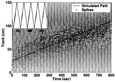
To illustrate the algorithm, we analyze first simulated spike train data based on the place cell model in Eq. 3.1, by using parameters consistent with the known spiking dynamics of hippocampal neurons. Simulation of the model in Eq. 3.1 was carried out by using a thinning algorithm, assuming an inhomogeneous Poisson process (22, 23). We assumed a 150-cm linear track with a rat running at a constant velocity of 25 cm/sec and simulated the spiking activity of a single place cell (Fig. 1). The simulated place field was directional; the cell fired only when the animal moved from the bottom to the top of the track (Fig. 1 Inset). During the 800-sec experiment, the place field parameters evolved linearly as follows: exp(α), the maximum spike rate grew from 10 to 25 spikes per sec; σ, the place field scale, expanded from 12 to 18 cm, and μ, the place field center, migrated from 25 to 125 cm. The spiking activity was designed to simulate the unidirectional migration, increase in scale, and increase in maximal firing rate characteristic of place cells for an animal running on a linear track (5, 10, 11).

Figure 1.

Simulated dynamics of a single place cell's spiking activity recorded from a rat running back and forth on a 150-cm linear track at a constant speed of 25 cm/sec for 800 sec. The vertical axis is space, and the horizontal axis is time. The vertical lines show the animal's path, and the dots indicate the location of the animal when the neuron discharged a spike. The spiking activity is unidirectional; the cell fires only when the animal moves from the top to the bottom of the track, as seen in the Inset. Simulations used an inhomogeneous Poisson model for Eq. 3.1. Over the 800 sec, the place field parameters evolved as follows: exp(α), the maximum spike rate grew from 10 to 25 spikes per sec; σ, the place field scale, expanded from 12 to 18 cm; and μ, the place field center, migrated from 25 to 125 cm. The solid diagonal line is the true trajectory of μ.

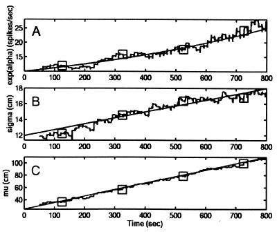
We applied our adaptive filter algorithm to the simulated data, updating the parameter estimates every 1 msec. The absolute values of the components in the dynamic gain are upper bounds on the changes in the components of θ at each step. By using the results of Mehta et al. (5), we computed average values of the dynamic gain vector and set the learning rate parameters at 10 times these average values to track rapid receptive field changes (10). We computed the initial parameter guesses as the maximum likelihood (ML) estimates based on the first 50 spikes (∼50 sec). For α, σ, and μ, the initial parameter estimates were close to the true values (Fig. 2 A–C). As a consequence, the adaptive algorithm begins to track all three parameters immediately, and the true and estimated trajectories agree over the entire simulation.

Figure 2.

True parameter trajectories and the adaptive estimates of parameter trajectories for the place field model in Eq. 3.1. The straight (wavy) line is (A). True (estimated) trajectory of the maximum spike rate, exp(α). (B) True (estimated) trajectory of the scale parameter, σ. (C) True (estimated) trajectory of the place field center, μ. Adaptive estimates were updated every 1 msec. Squares on the estimated parameter trajectories at 125, 325, 525, and 725 sec indicate the times at which the place fields in Fig. 3 are evaluated. The algorithm accurately tracked the temporal evolution of the model parameters.

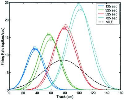
A comparison of the true and estimated place fields over time is illustrated in Fig. 3. The place field increases in height (maximum firing rate) and width with time. The algorithm shows good agreement between the true (dashed lines) and estimated (solid lines) place fields with unbiased tracking of all three parameters. The advantage of using an adaptive estimation algorithm is demonstrated by comparing the static ML place field estimate for the entire experiment with the adaptive estimates (Fig. 3). By ignoring the dynamics of the place field, the ML estimate incorrectly represents the field as a low-amplitude broad structure that spans the entire track. Static ML analyses ignore the plasticity in the place cell's spatial properties. A video presentation of this analysis is published as supporting information on the PNAS web site, www.pnas.org.

Figure 3.

Evolution of the true (dashed lines) and adaptive estimates (solid lines) of the place fields. The place fields are shown at 125 (blue), 325 (green), 525 (red), and 725 (aqua) sec. The black dashed line is the ML estimate of the place field based on all the spikes in the 800 sec. By ignoring the temporal evolution of the place field, the ML estimate gives a misleading description of the field's true characteristics, representing it incorrectly as a low-amplitude broad structure that spans the entire track.

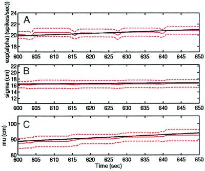
For an arbitrary set of parameters and an arbitrary learning rate, it is not given that the adaptive algorithm will track correctly, because our theoretical results in the Appendix give only the conditions necessary for tracking. Therefore, for the parameter values used in Fig. 1, we simulated 50 realizations of place cell data and applied the adaptive estimation algorithm to each data set to illustrate that the results in the simulated example in Figs. 1–3 are typical. At each update time point kΔ, we computed the mean and standard deviation of the 50 adaptively estimated parameters and used these to derive approximate 95% confidence intervals for the true parameter value at each time point. The results of this analysis (Fig. 4) agree closely with the single series simulations in Fig. 1. All the confidence intervals cover the true parameter trajectories. The averaged and true trajectories of exp(α) (Fig. 4A) and σ (Fig. 4B) are indistinguishable and show no bias, whereas the averaged trajectory of μ (Fig. 4C) is close to the true trajectory with a slight negative bias. This slight bias reflects the time lag in the estimation because the algorithm uses no model about the actual parameter trajectory to make a one-step-ahead prediction of the next parameter value prior to computing the updated estimate on the basis of newly recorded spiking activity. Overall, the simulation suggests that the algorithm tracks well.

Figure 4.

Simulation study of the adaptive filter algorithm (Eq. 3.3) by using 50 realizations of the place cell model in Eq. 3.1 and the parameters in Fig. 1. Only 50 sec of the full trajectories are displayed with expanded scales to aid visualization. The true trajectory (black solid line) is shown along with the average of the adaptive estimates of the trajectory (red solid line). Approximate 95% confidence bounds (red dashed lines) were computed for each parameter. (A) exp(α); (B) σ; and (C) μ. All true trajectories are within the 95% confidence bounds, and all estimated trajectories are close to the true trajectories.

Adaptive Analysis of Actual Place Receptive Field Dynamics.

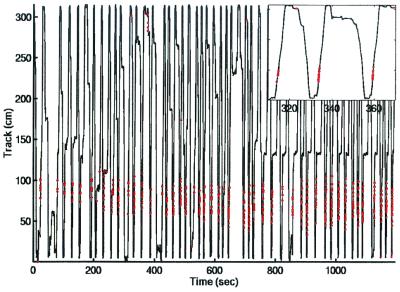
We applied the adaptive filter algorithm to an actual place cell spike train recorded from a rat running back and forth for 1,200 sec on a 300-cm U-shaped track (24). To display all the experimental data on a single graph, we show a linear representation of the track (Fig. 5). The actual trajectory is much less regular than the simulated trajectory in Fig. 1, because the animal stops and starts several times, and in two instances (50 and 650 sec) turns around shortly after initiating its run. On several of the upward passes, particularly in the latter part of the experiment, the animal slows as it approaches the curve in the U-shaped track at approximately 150 cm. The strong place-specific firing of the neuron is readily visible as the spiking activity occurs almost exclusively between 50 and 100 cm. The spiking activity of the neuron is entirely unidirectional as the cell discharges only as the animal runs up and not down the track (Fig. 5 Inset).

Figure 5.

Place-specific firing dynamics of an actual CA1 place cell recorded from a rat running back and forth on a 300-cm U-shaped track for 1,200 sec. The track was linearized to display the entire experiment in a single graph. The vertical lines show the animal's position, and the red dots indicate the times at which a spike was recorded. The Inset is an enlargement of the display from 320 to 360 sec to show the cell's unidirectional firing, i.e., spiking only when the animal runs from the bottom to the top of the track.

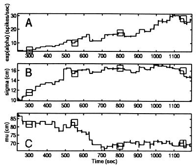
We applied the model (Eq. 3.1) and the adaptive filter algorithm (Eq. 3.3) to this actual spike train data, updating the estimates every 1 msec. We used the learning rate parameters chosen in the simulation study. The starting parameter estimates were the ML estimate computed from the first 50 spikes (∼200 sec). The trajectory of exp(α), the maximum spike rate, shows a steady increase from 3 to almost 30 spikes/sec over the 1,200 sec of the experiment (Fig. 6A). The increase is apparent in the raw data in Fig. 5. The scale parameter, σ, shows the greatest fluctuations during the experiment; it rises for the first 500 sec from 10 to 16 cm and fluctuates between 15 and 16 cm for the balance of the experiment (Fig. 6B). This fluctuation in scale is also readily visible in the spike train data in Fig. 5. The place cell center migrates over the first 700 sec from 85 to 65 cm and stays near 65 cm for the remainder of the experiment (Fig. 6C).

Figure 6.

Adaptive filter estimates of the trajectories. (A) Maximum spike rate, exp(α); (B) place field scale, σ; and (C) place field center μ. Adaptive estimates were updated at 1-msec intervals. The squares at 300, 550, 800, and 1,150 sec are the times at which the place fields are displayed in Fig. 7. The growth of the maximum spike rate (A), the variability of the place field scale (B), and the migration of the place field center (C) are all readily visible.

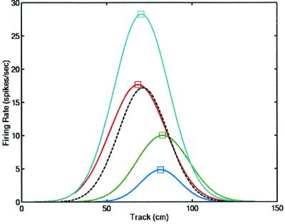
The evolution of the entire field is illustrated in Fig. 7 by plotting the instantaneous place field estimates at 300, 550, 800, and 1,150 sec. The sequence of place field estimates shows the time evolution of the cell's spatial receptive field. By contrast, the ML estimate based on the entire 1,200 sec of data obscures the temporal dynamics by overestimating (underestimating) the place field's spatial extent and underestimating (overestimating) its maximum firing rate at the end (beginning) of the experiment. This example shows that the dynamic of actual place cell receptive fields can be tracked instantaneously from recorded spiking activity. The migration of center and the growth in scale and in maximum firing rate are consistent with previous reports (5, 10). A video presentation of this analysis is published as supporting data on the PNAS web site, www.pnas.org, along with analyses of the spatial receptive field dynamics of three other CA1 hippocampal neurons.

Figure 7.

Estimated place fields at times 300 (blue), 550 (green), 800 (red), and 1,150 (aqua) sec. As in Fig. 3, the black dashed line is the ML estimate of the place field obtained by using all the spikes in the experiment. The ML estimate ignores the temporal evolution of the place field (see Fig. 3).

Our current analysis captures all the dynamic behavior of place cells with the exception of skewing. By construction, the place cell model in Eq. 3.1 cannot describe this behavior. To reliably track skewing along with the other dynamic features of the place cells, we reformulated our adaptive filter algorithm by using a spline-based model for the place field. A description of this model and an example of its application are also published as supporting information on the PNAS web site, www.pnas.org.

Discussion

We have presented an approach to analyzing neural receptive field plasticity by using a point process adaptive filter algorithm. The key to designing the algorithm was use of the instantaneous log likelihood (Eq. 2.4) of a point-process model as the criterion function in the instantaneous steepest descent formula (Eq. 2.5). The more commonly used quadratic criterion function has limited applicability to spike train data unless the point process time series can be well approximated by a continuous-valued process. The conditional intensity function (Eq. 2.1) completely defines the probability structure of a regular point process (18) and its instantaneous log likelihood. Therefore, specifying a conditional intensity function model of a neural spike train with a time-varying parameter provides a straightforward general prescription for constructing a point process adaptive filtering algorithm using instantaneous steepest descent.

Our adaptive filter algorithm offers important advantages over commonly used histogram-based methods for analyzing receptive field plasticity. Whereas histogram methods provide discrete snapshots of neural receptive fields in broad nonoverlapping time windows, our algorithm can track receptive field dynamics on a millisecond time scale. We find that videos rather than graphical displays offer the best means of studying receptive field plasticity with our methods (see data, www.pnas.org, and http://neurostat.mgh.harvard.edu). Our adaptive filter formally resembles certain algorithms in statistical learning theory (25). Unlike neural network-based learning algorithms (13, 14), our algorithm represents the relation between the stimulus and the neural response with a parametric model. It can begin tracking after a short initial estimation period (50–200 sec in our examples), because it does not require an extended training period to learn the salient characteristics of the neural system.

Our small simulation study suggests that the adaptive filter algorithm tracked well a set of parameter trajectories like those seen in actual hippocampal neurons. In our analysis of the actual place cell data, the spatial receptive fields migrated in the direction opposite the cell's preferred direction of firing relative to the animal's movement and increased in scale and maximum firing rate as in the average behavior described in previous reports (5, 10, 11). Place field migration was predicted by Blum and Abbott (11) on the basis of postulated asymmetric Hebbian strengthening of synapses between hippocampal neurons with overlapping place fields. Mehta et al. (5, 10) observed place field migration and skewing (10) in CA1 neurons, reporting their findings in terms of population summaries of place field characteristics averaged across cells. Our adaptive filter algorithm can track the temporal dynamics of place fields for individual cells. We successfully tracked the skewing seen in hippocampal place fields by using our adaptive filter with a spline to model the field's non-Gaussian spatial structure (supporting information, www.pnas.org).

Our results establish the feasibility of using adaptive signal processing methods to analyze neural receptive field plasticity. Further development of this work is needed to make these methods a useful practical tool for spike train data analysis. First, because neural activity in many brain regions, including the hippocampus, is not best modeled as a Poisson process (26, 27), applying the point process adaptive filter in the general (non-Poisson) framework in Eq. 2.8 is an important extension we are investigating. Second, the place field model should be extended to include covariates other than position that affect hippocampal spiking activity such as theta rhythm modulation, the animal's running speed, and phase precession (21). Third, our stability analysis established only the necessary condition of local stability for the case in which the parameter trajectories are time-varying around a constant true value. Global stability of our algorithm is currently being investigated. We chose ɛ on the basis of the estimated maximum change in the dynamic gain function (Eq. 2.8). Our adaptive filter estimates were insensitive to 50% changes in ɛ determined this way. The global stability analysis and further simulation studies will also help develop a systematic approach to choosing the learning rate parameters. Fourth, we are developing alternative point process adaptive filter algorithms analogous to the extended Kalman filter and recursive least-squares methods for continuous-valued data (15, 16). These approaches offer standard errors and confidence bounds for the estimated parameter trajectories. Finally, we are extending the point process goodness-of-fit measures developed by Brown and colleagues (19, 27) to assess overall agreement between spike trains and conditional intensity function models with time-varying parameters. These methods will provide an important measure of how reliably the adaptive algorithms perform in actual data analyses.

Future investigations with our point process adaptive filter algorithms will include a study of hippocampal place field formation as the animal learns a novel environment. We previously reported a decoding study of hippocampal place cell ensembles, which assumed the place field characteristics to be unchanged during the decoding stage of the analysis (19). We will reanalyze these data by using dynamically updated place field estimates computed from our adaptive filter algorithm.

Stability Analysis

To guarantee that our adaptive point process filter algorithm is capable of tracking time-varying changes in θ, it is necessary to analyze its stability properties. A global stability analysis of our algorithm is a major task that will be pursued in detail elsewhere. Here, we sketch an argument to show that our algorithm exhibits the less general but nevertheless important basic property of local stability. We show that: (i) our algorithm in Eq. 2.6 may be represented as a forced nonlinear time-varying stochastic dynamical system, (ii) the homogeneous (unforced) component of this stochastic system is locally stable by using averaging methods (15) to show that the associated averaged deterministic system is locally stable, and (iii) because the averaged system is locally stable, we conclude by the Hovering theorem that the corresponding homogeneous stochastic system is locally stable (15). By local stability, we mean that if θ(t) = θ₀, the homogeneous component of the stochastic dynamical system converges to θ₀ as t → ∞.

A Stochastic Dynamical System Representation of the Point Process Adaptive Filter Algorithm.

To simplify notation, we let λ_θ(t) = λ(t|H_t, θ(t)). We express Eq. 2.6 in its continuous time form

A.1

If we combine Eqs. 2.4 and A.1, then the instantaneous steepest descent algorithm has the general form

A.2

For any θ₀, we can re-express Eq. A.2 as

A.3

The term dN(t) − λ_θ0(t)dt is a martingale increment (roughly speaking, a white noise) (28), so that the second term on the right hand side of Eq. A.3 is a white noise forcing the homogeneous system

A.4

Averaging Methods and a Local Stability Analysis.

Given the homogeneous system in Eq. A.4, we proceed in two steps to analyze its local stability by using averaging methods (15). In step one, we approximate Eq. A.4 by a simpler averaged system, which is deterministic and whose local stability can be directly established. In step two, we use the Hovering theorem (15) to conclude that the system in Eq. A.3 is locally stable. The Hovering theorem provides conditions under which the stability of a stochastic system, such as Eq. A.3, may be inferred from the stability of its associated averaged deterministic system. We let θ̄(t) denote the variable of the averaged system. The averaged system associated with Eq. A.4 is defined as (15)

A.5

where f_av(θ̄(t)) = E[(λ_θ0(t) − λ_θ̄(t))(∂log λ_θ̄(t)/∂θ)], and the expectation is with respect to the marginal probability density of x(t). We expand Eq. A.5 in a Taylor series about θ₀ to obtain the linearized system

A.6

where A is the p × p matrix defined as A = −(∂f_av(θ̄(t))/∂θ)|_θ̄(t)=θ0 = E(λ_θ̄(t)(∂log λ_θ̄(t)/∂θ)((∂log λ_θ̄(t)/∂θ))′), and p is the dimension of θ̄(t). We have local exponential stability if θ̄(t) is uniformly bounded and A is positive definite, i.e., c′Ac > 0 for any vector c ≠ 0. Showing that θ̄(t) is uniformly bounded is straightforward by using Lyapounov methods (15). We omit this technical point. Local exponential stability is a property of the system in Eq. A.6, because for any c ≠ 0, c′Ac = E[λ_θ̄(t)(c′(∂log λ_θ̄(t)/∂θ))²] > 0, provided the marginal probability density of x(t) is nondegenerate. Therefore, the averaged deterministic system in Eq. A.5 is locally stable. Local stability of the homogeneous stochastic system in Eq. A.4 now follows by simply verifying that it satisfies the conditions of the Hovering theorem (15).

References

- 1.Donoghue J P. Curr Opin Neurobiol. 1995;5:749–754. doi: 10.1016/0959-4388(95)80102-2. [DOI] [PubMed] [Google Scholar]
- 2.Weinberger N M. Curr Opin Neurobiol. 1993;3:570–577. doi: 10.1016/0959-4388(93)90058-7. [DOI] [PubMed] [Google Scholar]
- 3.Pettet M W, Gilbert C D. Proc Natl Acad Sci USA. 1992;89:8366–8370. doi: 10.1073/pnas.89.17.8366. [DOI] [PMC free article] [PubMed] [Google Scholar]
- 4.Jog M S, Kubota Y, Connolly C I, Hillegaart V, Graybiel A M. Science. 1999;286:1745–1749. doi: 10.1126/science.286.5445.1745. [DOI] [PubMed] [Google Scholar]
- 5.Mehta M R, Barnes C A, McNaughton B L. Proc Natl Acad Sci USA. 1997;94:8918–8921. doi: 10.1073/pnas.94.16.8918. [DOI] [PMC free article] [PubMed] [Google Scholar]
- 6.Merzenich M M, Nelson R J, Stryker M P, Cynader M S, Schoppmann A, Zook J M. J Comp Neurol. 1984;224:591–605. doi: 10.1002/cne.902240408. [DOI] [PubMed] [Google Scholar]
- 7.Kaas J H, Merzenich M M, Killackey H P. Annu Rev Neurosci. 1983;6:325–356. doi: 10.1146/annurev.ne.06.030183.001545. [DOI] [PubMed] [Google Scholar]
- 8.Gandolfo F, Li C, Benda B J, Schioppa C P, Bizzi E. Proc Natl Acad Sci USA. 2000;97:2259–2263. doi: 10.1073/pnas.040567097. . (First Published February 11, 2000; 10.1073/pnas.040567097) [DOI] [PMC free article] [PubMed] [Google Scholar]
- 9.O'Keefe J, Dostrovsky J. Brain Res. 1971;34:171–175. doi: 10.1016/0006-8993(71)90358-1. [DOI] [PubMed] [Google Scholar]
- 10.Mehta M R, Quirk M C, Wilson M A. Neuron. 2000;25:707–715. doi: 10.1016/s0896-6273(00)81072-7. [DOI] [PubMed] [Google Scholar]
- 11.Blum K I, Abbott L F. Neural Comput. 1996;8:85–93. doi: 10.1162/neco.1996.8.1.85. [DOI] [PubMed] [Google Scholar]
- 12.Abbott L F, Varela J A, Sen K, Nelson S B. Science. 1997;275:220–223. doi: 10.1126/science.275.5297.221. [DOI] [PubMed] [Google Scholar]
- 13.Ripley B. Pattern Recognition and Neural Networks. Cambridge, U.K.: United Press; 1996. [Google Scholar]
- 14.Hertz J A, Krogh A, Palmer R. Introduction to the Theory of Neural Computation. Reading, MA: Addison–Wesley; 1991. [Google Scholar]
- 15.Solo V, Kong X. Adaptive Signal Processing Algorithms: Stability and Performance. Upper Saddle River, NJ: Prentice–Hall; 1995. [Google Scholar]
- 16.Haykin S. Adaptive Filter Theory. Englewood Cliffs, NJ: Prentice–Hall; 1996. [Google Scholar]
- 17.Snyder D, Miller M. Random Point Processes in Time and Space. New York: Springer; 1991. [Google Scholar]
- 18.Daley D, Vere-Jones D. An Introduction to the Theory of Point Process. New York: Springer; 1988. [Google Scholar]
- 19.Brown E N, Frank L M, Tang D, Quirk M C, Wilson M A. J Neurosci. 1998;18:7411–7425. doi: 10.1523/JNEUROSCI.18-18-07411.1998. [DOI] [PMC free article] [PubMed] [Google Scholar]
- 20.McNaughton B L, Barnes C A, O'Keefe J. Exp Brain Res. 1983;52:41–49. doi: 10.1007/BF00237147. [DOI] [PubMed] [Google Scholar]
- 21.O'Keefe J, Recce M L. Hippocampus. 1993;3:317–330. doi: 10.1002/hipo.450030307. [DOI] [PubMed] [Google Scholar]
- 22.Lewis P A W, Shedler G S. Naval Res Logistics Quart. 1978;26:403–413. [Google Scholar]
- 23.Ross S. Introduction to Probability Models. San Diego: Academic; 1993. [Google Scholar]
- 24.Frank L M, Brown E N, Wilson M A. Neuron. 2000;27:169–178. doi: 10.1016/s0896-6273(00)00018-0. [DOI] [PubMed] [Google Scholar]
- 25.Cherkassky V, Mulier F. Learning from Data: Concepts, Theory and Methods. New York: Wiley; 1998. [Google Scholar]
- 26.Gabbiani F, Koch C. In: Methods in Neuronal Modeling. Koch C, Segev I, editors. Cambridge, MA: MIT Press; 1998. pp. 313–360. [Google Scholar]
- 27.Barbieri R, Quirk M C, Frank L M, Wilson M A, Brown E N. J Neurosci Methods. 2001;105:25–37. doi: 10.1016/s0165-0270(00)00344-7. [DOI] [PubMed] [Google Scholar]
- 28.Brémaud P. Point Processes and Queues: Martingale Dynamics. Berlin: Springer; 1981. [Google Scholar]
Associated Data
This section collects any data citations, data availability statements, or supplementary materials included in this article.