Superpixel-based and boundary-sensitive convolutional neural network for automated liver segmentation

Abstract

Purpose

Segmentation of liver in abdominal computed tomography (CT) is an important step for radiation therapy planning of hepatocellular carcinoma. Practically, a fully automatic segmentation of liver remains challenging because of low soft tissue contrast between liver and its surrounding organs, and its highly deformable shape. The purpose of this work is to develop a novel superpixel-based and boundary sensitive convolutional neural network (SBBS-CNN) pipeline for automated liver segmentation.

Method

The entire CT images were first partitioned into superpixel regions, where nearby pixels with similar CT number were aggregated. Secondly, we converted the conventional binary segmentation into a multinomial classification by labeling the superpixels into three classes: interior liver, liver boundary, and non-liver background. By doing this, the boundary region of the liver was explicitly identified and highlighted for the subsequent classification. Thirdly, we computed an entropy-based saliency map for each CT volume, and leveraged this map to guide the sampling of image patches over the superpixels. In this way, more patches were extracted from informative regions (e.g., the liver boundary with irregular changes) and fewer patches were extracted from homogeneous regions. Finally, deep CNN pipeline was built and trained to predict the probability map of the liver boundary.

Results

We tested the proposed algorithm in a cohort of 100 patients. With 10-fold cross validation, the SBBS-CNN achieved mean Dice similarity coefficients of 97.31±0.36% and average symmetric surface distance of 1.77±0.49mm. Moreover, it showed superior performance in comparison with state-of-art methods, including U-Net, pixel-based CNN, active contour, level-sets and graph-cut algorithms.

Conclusion

SBBS-CNN provides an accurate and effective tool for automated liver segmentation. It is also envisioned that the proposed framework is directly applicable in other medical image segmentation scenarios.

1. Introduction

The accurate segmentation of liver is important not only for radiation therapy planning, but also for follow-up evaluations (Mharib et al., 2012). In current clinical practice, manually delineation is time-consuming and may suffer from inter- and intra-operator variations (Dou et al., 2017). While several methods have been proposed (Hoogi et al., 2017; Li et al., 2016; Dou et al., 2017; Zheng et al., 2017), automated liver segmentation remains challenging. Briefly, the existing liver segmentation methods can be subdivided into two categories: model-based or learning-based methods. Among the model-based methods, atlas-based models (Li et al. 2017), graphical models (Wu et al., 2016; Luo et al., 2013), and deformable models(Chartrand et al., 2016; Li et al., 2015) have been proposed. Despite that the involvement of sophisticated registration and parametric modeling steps, the results obtained from the methods may still be inaccurate. In learning-based segmentations, handcrafted features are extracted first and classification models are then employed to train and label the target images (Zheng et al., 2016). A major shortcoming of the learning-based methods is that they require careful feature engineering to achieve good performance.

Recently, deep learning has emerged as a powerful technique for medical image analysis (Litjens et al., 2017; Shen et al., 2017; Ibragimov and Xing, 2017; Bibault et al., 2016; Esteva et al., 2017; Long et al., 2017). In most published applications, convolutional neural network (CNN) is used as a pipeline to automatically generate discriminative features for further supervised learning. For conventional use of CNN in computer vision, a single class label vector is associated with an individual image for classification purpose. In contrast, for object segmentation, the desired output is a pixel-wise class probability map. A few studies have been made to develop CNN pipelines for medical image segmentation, including segmentations of liver (Hu et al., 2016), prostate (Guo et al., 2016), isointense stage brain tissues (Zhang et al., 2015), brain tumor (Pereira et al., 2016), and pancreas (Roth et al., 2015). However, most of these existing deep learning approaches are based on pixelated CNN and they suffer from the limitations of computational efficiency and disturbances from noises. Moreover, the information for overlapping pixel-based patches may be redundant. In order to go beyond the local patch-based CNN analysis, a recent studies ( Ronneberger et al., 2015; Milletari et al., 2016) proposed a U-Net network architecture or its variant model to directly analyze the whole imaging data, which takes full advantage of global patterns within the images. Han (2016) proposed a DCNN method based on the U-Net and ResNet, which ranked the first for the LiTS challenge at the time of the ISBI 2017 and showed the best performance on the recent thoracic auto-segmentation challenge at AAPM 2017. In general, these methods are computationally costly due to high memory requirement of the model during training and not easily applicable for 3D medical image, which is at least two orders of magnitude computation burden than superpixel-based CNN segmentation method due to each pixel convolutional calculation in U-Net.

Superpixel algorithm groups pixels with similar properties into perceptually meaningful atomic regions while considering spatial constraints. Additionally, it preserves the edge information of the original image during the process of enhancing the local consistency. He et al (2015) recently proposed a superpixel CNN approach by re-arranging superpixels, which however required features extraction. Furthermore, the boundary between the target organ and its neighboring tissues may be ambiguous due to potentially limited contrast in medical images. Therefore, the pixel-based patch-wise or fully CNN may still be challenging in accurately delineatation of the liver organ boundary due to the restriction in memory demanding and highly imbalanced class training set (Chen et al., 2017; Ghafoorian et al., 2017; Han X, 2017). The probability prediction result does not necessarily represent the final segmentation. From previous studies, deep learning methods are usually used to generate the prior probability map of subject of interest as initialization, and further integrate with model-based models such as Graph-cuts (Lu et al., 2017), Level-sets (Cha et al., 2016), Surface evolution (Hu et al., 2016) and Markov random fields (Ibragimov and Xing, 2017) to improve the consistency of the obtained results.

Here, we presented a CNN pipeline for fully automatic liver segmentation. Compared with the existing algorithms, there are two major novelties in the proposed framework:

1. We transform classic binary segmentation tasks (i.e., liver or non-liver) into a multinomial classification problem. In other words, we explicitly labeled the boundary as a separate class. By doing so, more learning power is given to boundary, which can significantly increase the detection accuracy. Many previous deep learning algorithms served as the initial contour generation for the subsequent shape-based algorithms (e.g., level-set). Our method explicitly addresses the issues of boundary prediction problem and provides more information on edge for network perception. As thus, it can delineate liver edges without further post-processing.

2. Our CNN framework is based on superpixels rather than on individual pixels. Moreover, we utilize entropy-based saliency map to guide the patch sampling where more patches are extracted from more informative regions. By eliminating patches that are redundant and only keeping informative ones, the training patch size is decreased by at least two orders of magnitude, leading to significantly improved computational efficiency and robustness.

The remaining of this article is organized as follows. In section 2, we describe the details of the proposed framework and evaluation tests. The results are presented in section 3, followed by some discussions in section 4 and concluding remarks in section 5.

2. Materials and methods

The overview of the proposed framework is depicted in figure 1. In the training stage, we first converted the binary ROI (region-of-interest) contours (liver in this study) into a multinomial map. Meanwhile, we obtained a set of superpixels and the saliency maps from CT images. Under the guidance of saliency maps, we extracted patches containing superpixels and assigned them the class labels, i.e., interior liver, liver boundary and non-liver background. A six-layer CNN network was then trained with these image patches and their labels. In the test stage, we applied the trained model to predict the class label of an independent dataset. In details, the image patches that cover all superpixels from individual patients were analyzed and assigned the probability for three classes. The probability maps were integrated into the final segmentation result.

Figure 1.

Schematic diagram of the SBBS-CNN architecture used in this study

2.1. Imaging dataset and preprocessing

The public dataset from LiTS - Liver Tumor Segmentation Challenge (ISBI2017) were used for this study. The dataset contains 100 abdomen contrast CT scans. More details of this dataset and imaging protocols can be found online (https://competitions.codalab.org/competitions/17094). Briefly, the in-plane matrix is 512×512 with resolution ranged from 0.45mm to 0.98mm and slice numbers vary from 75 to 987 with resolution ranged from 0.45mm to 5mm. All liver segmentations were carefully prepared and visually checked by a radiation oncologist (F.H., with 23 years experiences in radiation therapy).

We first transfer data into the same physical resolution space 1×1×1 mm using coordinate transform and bilinear interpolation. A Gaussian filter with Sigma of 0.5 in voxels is used to de-noise the input CT data for enhance image contrast (Pawar et al, 2017). Hence, we set the intensity range as [−200,200] in our experiments, because the Hounsfield scale is +40 to +60. When CT intensity value is higher than 200, the intensity is set to 200, likewise, the intensity is set to −200 when intensity is less than −200. We further scale the window value in a range of zero to unity.

2.2. Superpixel-based boundary sensitive patch selection guided by saliency map

The term of superpixel (Ren and Malik, 2003) is used to describe a group of pixels similar in interested low-level feature space. It has several known advantages for image segmentation. Firstly, it can be used to accelerate computationally demanding algorithms without obvious information loss. Second, the regular shape bricks preserve the main connection relationships within images. Although the superpixel-based over-segmentation gives a semantically meaningful representation of original images, which image characteristics are expressed by using few superpixels with similar color, brightness and texture instead of massive pixels (Tian et al., 2016).

Conventionally, the patches are extracted iteratively based on the predefined grid that superimposed on the original image. Thus, redundant patches are extracted for further network analysis, which can significantly deteriorate following analysis due to learning from imbalanced data. To overcome this, we generated the superpixels to guide the image patches extraction. In details, Simple Linear Iterative Clustering (SLIC) method (Achanta et al., 2012) was adopted to obtain superpixels. Moreover, SLIC algorithm performs better in adhering to image boundaries, speed, and memory efficiency compared with five state-of-the-art superpixel algorithms (Achanta et al., 2012). However, distinct from nature images, CT images can be more heterogeneous. In regions possessing similar CT numbers, it remains challenging to have the boundary properly covered by superpixels, which is shown in figure 4, especially for the superpixels at the border of the liver that usually suffered from the edge leakage. Therefore, the training patch selection has a great impact on training the following segmentation model.

Figure 4.

Examples of superpixel segmentations produced by different numbers of superpixel: The top row is the different numbers of superpixels, from (a)–(c) is 100, 2000, 5000 superpixels respectively. The image data inside the red box in (a)–(c) are displayed in the top row.

As illustrated in figure 2(b), we obtained a set of subregions S = (S₁, S₂, … S_i, …, S_M), i ∈ (1, M) using SLIC, where M is the number of superpixels. The i-th superpixel is composed of a set of N pixels S_i = {m_i(1), …, m_i(j), …, m_i(N)} with m_i(j) ∈ I, I is the CT slice image, If every pixel m_i(j) of superpixel S_i belongs to labeled liver class, the superpixel S_i is labeled as liver class. Otherwise, there is a certain proportion of pixels inside the superpixel S_i, i ∈(1, M) belongs to liver, we assign it as the boundary class. The superpixels that do not contain any liver pixel are assigned as background class.

Figure 2.

An example of superpixel-based patch candidates sample. (a) original CT slice image after preprocessing, (b) illustration of the superpixel and patch definition, (c) sample superpixel candidates. Superpixel with an entropy value greater than 1.5 are denoted by green color and selected in patch extraction.

Given a superpixel map, we also measured the information contained within each superpixel by computing a saliency map based on Shannon entropy (Mylona et al., 2012), as figure 3(c). Here, we selected the superpixel with the mean entropy value greater than 1.5 to be the training patches. Redundant background patches and non-informative patches were excluded to improve the robustness and efficiency of the network. The final sample candidate patches with entropy value larger than 1.5 were shown in green in figure 3(c).

Figure 3.

Demonstration of superpixel-based patches extraction: (a) background patches outside of the liver area. (b) liver patches with all pixel inside the patch. (c) superpixel-based boundary patches.

Given a CT slice image I and segmented regions (superpixel) S =(S₁, S₂, … S_i, …, S_M), each image patch P_k ∈ R^h×w with its size in height h and width w and value R in interval [0,1] can be obtained from centroid of each superpixel S_i. Our aim here is to predict class labels for individual superpixels denoted as ℒ ={ℒ₁, ℒ₂,…, ℒ_M}, where ℒ_i =0, ℒ_i =1, ℒ_i =2 represents non-liver background, liver and liver boundary respectively. In this study, we chose the patch size to be 32×32, which will be explained in the following discussion section. The detailed illustration for three class are shown in Figure 4. The patches were obtained from centroid of each superpixels. The k-th training patch class label based on pixel-level ground truth is obtained by the following equation:

$$P_k(t_k)=\{\begin{array}{cc}0& if{m}_k(j)\in \mathcal{L}\{0\}orif\frac{m_k(j)\in \mathcal{L}\{1\}}{m_k(j)\in \mathcal{L}\{0\}+m_k(j)\in \mathcal{L}\{1\}}\le \mathrm{\theta }\\ 1& if{m}_k(j)\in \mathcal{L}\{1\}\\ 2& if\frac{m_k(j)\in \mathcal{L}\{1\}}{m_k(j)\in \mathcal{L}\{0\}+m_k(j)\in \mathcal{L}\{1\}}>\mathrm{\theta }\end{array}$$ (1)

where m_k(j) ∈ P_k denotes the j-th pixel located within the k-th patch, t_k is the k-th patch class label. Here, the “liver patch” is defined as a superpixel that all of its pixels are located inside the hand-outlined liver. When the ratio of area labeled as liver in a patch (m_k(j) ∈ ℒ{1}) to the total are of the patch (m_k(j) ∈ ℒ{0} + m_k(j) ∈ ℒ{1}) is over θ, it is considered as a “boundary patch”, as illustrated in figure 3(c). This makes the following network more sensitive to the boundary and facilitates the detection of the edge.

Intuitively, the number and size of superpixel N_sp would have important impact on subregion extraction. The selection of these parameters is generally empirical. If a large number of superpixels are extracted, the superpixels would well adhere to boundary, but the computation efficiency is greatly reduced. In the opposite case, increased under-segmentation error would be resulted. As illustrated in figure 4, large size superpixels will leak into the boundary, when the number of superpixels is less than 500. If the right amount of superpixels is selected, the liver boundary can be discretized properly. Here, we measured standard deviation of CT numbers inside each superpixel to determine the optimal number of superpixels.

2.3. Superpixel-based boundary-sensitive CNN (SBBS-CNN)

CNN is an architecture composed of convolution operator and pooling operator, which makes the best of local spatial correlation information and drastically reduces the number of parameters using their weight sharing. Because end-to-end trained CNN enables the network to extract high level representation automatically without manually selected features, the CNN has become ubiquitous for medical image analysis and shown to be very powerful.

Here, we tailored a popular CNN architecture known as Cifarnet (Krizhevsky and Hinton, 2009) to compute the superpixel probability maps Y(s_i|P_si). where s_i is the i-th superpixel, P_si is a patch at the s_i-th superpixel. The detailed network architecture is shown in figure 1. The CNN involves 6 layers: 2 layers for convolution operation, 2 layers for pooling operator, 1 layer for full connections and 1 layer for softmax prediction. In details, the convolutional layers are operators based on a group of filter banks with K kernels 𝒲 ={W₁, W₂, …, W_K} and subsequently biases ℬ ={b₁, …, b_k} are added. Let ℱ_k represent feature map based on superpixel patches, the output of each convolution layer can be defined as:

$${\mathcal{F}}_k^l=f(W_1^{l-1}\otimes {\mathcal{F}}_k^{l-1}+b_k^{l-1})$$ (2)

where f(·) is an element-wise non-linear transform, here we choose tangent functions tanh for each layer computation, because tanh can produce better a result than sigmoid that has gradient vanishing problem and computation burden (Jarrett et al., 2009).

The pooling layer is typically combined with convolution layer, which downscales the image to reduce the number of weight parameters. The redundant features can be made more compact and invariant to small insignificant details change. We used max-pooling in our network, which outputs the maximum value of each feature map within a predefined neighborhood. We also added a regularization term to prevent overfitting after each pooling layer, which is a nonlinear operator to transform the data. Here, we applied local response normalization scheme with Rectifier linear units (ReLU) (Krizhevsky et al., 2012). The response-normalized activity $b_{x,y}^i$ is defined as:

$$b_{x,y}^i=a_{x,y}^i{\left(k+\alpha {\mathrm{\sum }}_{j=max(0,i-n/2)}^{min(K-1,i+n/2)}{\left(a_{x,y}^i\right)}^2\right)}^{-\beta }$$ (3)

where $a_{x,y}^i$ is an activity of a neuron computed by non-linear transformation using tangent functions. The hyper-parameters k, α,β,n are constants whose values are determined empirically, more details can be found in (Krizhevsky et al. 2012).

In the classification layer, we used softmax to map the sequence map to a posterior over three classes. Softmax is a generalization of the logistic function that “squashes” a K-dimensional vector z of arbitrary real values to a K-dimensional vector $\mathrm{\sigma }{(\mathrm{Z})}_j=\frac{e^{z_j}}{{\mathrm{\sum }}_{k=1}^K{e}^{z_k}}$ of real values in the range (0, 1) that add up to 1.

For the model training, we trained the network to optimize the weight variables and bias values based on cross-entropy. The cross-entropy loss function is defined as

$$H(t_k,{\widehat{t}}_k)=-[t_{k}log({\widehat{t}}_k)-(1-t_k)\text{log}(1-{\widehat{t}}_k)]$$ (4)

and Adaptive Moment Estimation (Adam) optimization method (Kingma et al 2015) has been performed to minimize the loss function (4), which is a first-order gradient-based optimization method. In the end, we estimated convolution kernels 𝒲 ={W₁, W₂, …, W_K} and bias values ℬ ={b₁, b₂, …, b_K}.

In independent validation stage, we first extracted superpixel-based patches. The trained network was then used to infer the liver, liver boundary and background probability maps. In order to avoid over-segmentation, we firstly aggregate the liver and boundary probability Y(s_i|P_si) to form a probability map, and a threshold was then learned to reinforce the prediction probability to eliminate false positive objects. Any local maximum probability value less than the pre-chosen threshold is defined as background. Finally, we applied open and close morphology processing with disk-shaped structuring element to smoothen the edge of segmentation.

2.4. Training data augmentation and training details

Data augmentation is an essential step to enable the network the desired invariance and robustness properties. This is a process of generating new samples from original CT data, with automatic adjustment to the cases with a different orientation to make SBBS-CNN more robust to rotation-variant and noise disturbing. Here, random brightness and random right and left flip have been performed on superpixel-based patches. Because it is challenging to locate the edge in liver segmentation, we increased the numbers of liver boundary training set using 4-neighborhood connection around the centroid of the superpixel. Five patches will be extracted for boundary patches defined by formula (1). In total, approximately 1.6 million superpixel-based patches are extracted from the cases in the training set to depict background, liver, and boundary.

We initialized all weights using truncated normal distribution with mean 0 and standard deviation 0.05, with a constant 0.1 given to all biases. The detailed configuration of Tensorflow for the SBBS-CNN model is listed in Table 1.

Table 1.

Parameters configuration for SBBS-CNN

epoch	Learning rate	Decay of moving average	Weight decay
20000	0.1	0.9	0.004
60000	0.01	0.9	0.004
100000	0.001	0.9	0.004

2.5. Performance evaluation

In quantitatively comparing with the manual segmentation and validating the performance of the proposed method, we utilized five metrics to evaluate the SBBS-CNN results. We also compared the results with the state-of-art CNN model (Dong et al., 2017) and some representative model-based methods, including active contour Chan-Vese segmentation (Pascal et al, 2012), Graph-cuts (Wu et al., 2016, Jirik et al., 2013) and level-sets (Yushkevich et al., 2006 ).

The active contour Chan-Vese segmentation is based on level sets that are evolved iteratively to minimize an energy¹ (Pascal et al, 2012), In this paper, we used open source code scikit-image for liver segmentation. Graph cuts (Wu et al., 2016; Jirik et al., 2013) segmentation is a graph-based model method which minimizes the energy function via the max-flow/min-cut algorithm. We have used the python version opensource code for the study². Level-sets ³ (Yushkevich, 2006) is segmentation techniques based on partial differential equations (PDE), i.e. progressive evaluation of the differences among neighboring pixels to find object boundaries. Ideally, the algorithm converges to the boundary of the object where the differences are the highest, which have been integrated in opensource software ITK-SNAP.

With the manual contours as the gold standard, Dice Similarity Coefficient (DSC) is used to measure the similarity of segmentation masks. In terms of vector operations over binary contours A and B, DSC is given by:

$$\text{DSC}(\mathrm{A},\mathrm{B})=\frac{2\mid A\cap B\mid }{\mid A\mid +\mid B\mid }$$ (5)

If A and B is the same, the DSC score value is 1. Volume Overlap Error (VOE) is the complement of the Jaccard coefficient:

$$\text{VOE}(\mathrm{A},\mathrm{B})=1-\frac{\mid A\cap B\mid }{\mid A\cup B\mid }$$ (6)

Relative Volume Difference (RVD) is a relative difference between two objects

$$\text{RVD}(\mathrm{A},\mathrm{B})=\frac{\mid B\mid -\mid A\mid }{\mid A\mid }$$ (7)

In order to calculate the distance error between two input volumes, we use Average Symmetric Surface Distance (ASD) and maximum surface distance (MSD) metrics.

2.6. Computing platform

The proposed SBBS-CNN algorithm was implemented in the framework of Tensorflow version 1.0 (Google, 2017) using Python. The computation was done on a Windows 10 personal computer (PC) with an Intel i7-7700K CPU (4.2GHz, and 32GB memory) and Nvidia GPU GeForce GTX1070.

3. Results

3.1. Segmentation results from proposed SBBS-CNN

Figure 5 illustrates the segmentation results of the proposed method on three representative examples. The left column (figure 5(a)) shows original image slices after preprocessing using Hounsfield window and filter. To get a better visual understanding of the computation procedure, the prediction probability map of the liver (figure 5(b) and liver boundary (figure 5(c)) are visualized. Figure 5(d) is the fusion map of liver and boundary probability. The liver and liver boundary have been inferred accurately. Finally, we used a simple open and close morphology operation to optimize fusion probability map. The approach generated results in excellent agreement with manual segmentation.

Figure 5.

Examples of three liver segmentation cases displayed from the top to bottom. From left to right are: (a) original transversal 2D slice after data augmentation. (b) inner liver prediction probability map. (c) liver boundary prediction probability. (d) fusion probability map from liver and liver boundary probability map. (e) the final segmentation results, the yellow line is the outline of manual segmentation, and the red area indicates the results obtained using SBBS-CNN.

3.2. Quantitative evaluation of proposed SBBS-CNN

We used 10-fold cross validation to measure the performance of the proposed method. The patches in all experiments are extracted from planes of the CT image. The segmentation results are shown in table 2. The proposed approach yielded average DSC, RVD, VOE, ASD and MSD of 97.31±0.36%, 1.97±1.70%, 5.24±0.69%, 1.77±0.49mm, 13.03±5.71mm, respectively.

Table 2.

Quantitative evaluation of SBBS-CNN using CT images (ISBI challenge)

Vol No.(#)	DSC(%)	RVD(%)	VOE(%)	ASD(mm)	MSD(mm)
AVG	97.31	1.97	5.24	1.77	13.03
SD	0.36	1.70	0.69	0.49	5.71

In addition, we compare the proposed boundary-aware segmentation concept with the standard binary segmentation. As observed in Table 3, SBBS-CNN yields mean ASD of 1.77 and MSD of 13.03. Thus, it is obvious that our method can provide more precise contour delineation with smaller ASD and MSD value. Moreover, the mean DSC is 97.31%. The proposed SBBS-CNN improves the performance of edge detection.

Table 3.

Comparison between binary and multinomial segmentation with SBBS-CNN, all of the results are mean of evaluation set.

Number of Classes	DSC(%)	RVD(%)	VOE(%)	ASD(mm)	MSD(mm)
3	97.31±0.36	1.97±1.7	5.24±0.69	1.77±0.49	13.03±5.71
2	94.74±1.85	−3.92±5.31	9.95±3.29	2.99±1.10	28.86±14.39

To show that the proposed method is more efficient in memory usage and segmentation quality over the representative pixel-based CNN such as UNET (Dong et al., 2017), FCN+CRF (Zhao et al., 2016) and pixel-based CNN method with random patch selection, we applied random sampling 2000 patches of each case for pixel-based CNN to generate training set with the same number of superpixel-based patch set. In the comparison, experiments were done on the same training and test dataset using the same computing platform. As demonstrated in the Table 4, SBBS-CNN gives the best result with DSC 97.31 while using the mean evaluation time 7.22 s for each case. Qualitative comparisons are shown in figure 6.

Table 4.

Comparison of different CNN segmentation methods

Patch size	DSC(%)	RVD(%)	VOE(%)	ASD(mm)	MSD(mm)	Training time(hr)	Evaluation time(s)
UNET	86.40±6.33	−9.40±15.76	23.44±9.08	10.15±5.05	43.13±16.30	24.69	0.29
Pixel-based CNN	88.83±7.73	−10.60±7.01	19.37±11.49	8.9±12.75	40.31±39.68	5.3	1184.55
FCN+CRF	92.59±1.76	−8.26±5.95	13.74±3.01	4.44±1.47	23.14±9.42	5.3	0.20
SBBS-CNN	97.31±0.36	1.97±1.7	5.24±0.69	1.77±0.49	13.03±5.71	2.2	7.22

Figure 6.

Three views of liver segmentation cases displayed from the top to bottom. From left to right are: (a) original transversal 2D slice after data augmentation. (b) ground truth. (c) our proposed method. (d) pixel-based CNN method. (e) U-Net model segmentation.

3.3. Comparison with conventional model-based segmentation techniques

We compared the performance of SBBS-CNN with the conventional method: active contour Chan-Vese segmentation (Pascal, 2012), Graph-cuts (Wu et al., 2016) and level-sets (Yushkevich et al., 2006 ) on the same training and testing sets. Table 5 summarizes the results from different approaches. It is observed that the proposed method is better than the traditional model-based method as measured by all metrics. Figure 7 shows three examples of visualization results. From the corresponding zoomed parts (Figure 7(d)–(e)), the segmentation results obtained by the proposed method are clearly better than other methods and agreed well with manual delineation contour.

Table 5.

Comparison of different segmentation methods

Patch size	DSC(%)	RVD(%)	VOE(%)	ASD(mm)	MSD(mm)
Active contour	96.29±1.59	3.14±5.97	7.12±2.89	2.49±1.36	19.05±16.34
Level-sets	95.55±2.62	5.39±8.58	8.41±4.71	3.41±1.65	34.75±16.00
Graph-cuts	96.74±1.95	4.34±4.25	6.25±3.54	2.39±1.86	20.26±13.50
3-class SBBS-CNN	97.31±0.36	1.97±1.7	5.24±0.69	1.77±0.49	13.03±5.71

Figure 7.

Examples of SBBS-CNN segmentation results in comparison with other approaches on the testing set. The ground-truth is denoted in yellow, active contour, graph-cut, level-set, and SBBS-CNN are plotted in blue, cyan, green, and red, respectively. From left to right are (a)–(c) transverse slice of three cases. The corresponding zoomed parts in the green boxes are demonstrated in (d)–(e).

4. Discussion

We have proposed a fully automated deep learning framework for image segmentation. This work contributes to the field of image analysis in a few aspects. First, we combined the superpixel with saliency map as a replacement for the pixel-grid to substantially improve computational efficiency and segmentation robustness. For example, we would need to extract 262144 patches with window-sliding of 1 pixel offset for a 512×512 CT image slice, and in contrast here, only < 2,000 informative patches are required for superpixel-based approach, which is at least two orders of magnitude less. Furthermore, instead of using massive pixels, the supervoxel scheme presents a concise representation/characterization of an image. Practically, the introduction of superpixel is to simplify the search space so that image segmentation can be achieved more efficiently with an end-to-end trained CNN. In this approach, the typical properties of the basic pixels in the context of contours of the structures, such as spatial topology, structure, homogeneity, and isometric information, are preserved effectively. Thus, there is no compromise in spatial resolution of the resultant segmentation. In this study, the influence of different patch sizes on the performance of segmentation was also investigated (table 6). In our experiments, different patch sizes were first extracted from the same dataset, and the SBBS-CNN model was then trained for each group of patch size. The same metric was used to score the effect of patch size for segmentation. When the patch size is small, it cannot cover sufficient neighborhood contexture. On the other hand, if the patch size is too large, more redundant information is involved in the training set, which would not only degrade CNN performance, but also increase the calculation burden. We found that the optimal patch size is around 32×32 for liver segmentation.

Table 6.

Patch size dependence of SBBS-CNN liver segmentation

Patch size	DSC(%)	RVD(%)	VOE(%)	ASD(mm)	MSD(mm)	Time(s)
16×16	93.17±4.76	−0.44±9.87	12.48±7.68	11.91±27.02	48.41±64.90	7.32
24×24	95.38±1.41	−2.04±4.02	8.8±2.55	2.74±1.07	24.67±14.21	7.23
32×32	97.31±0.36	1.97±1.7	5.24±0.69	1.77±0.49	13.03±5.71	7.26
64×64	74.22±11.28	70.8±57.98	39.94±13.21	29.73±20.69	93.85±55.61	7.22

Secondly, we converted the classic binary segmentation into a multinomial task to explicitly adapt to patch-based CNN algorithm. We explicitly labeled the boundary into a separate class, as shown in figure 8. Compared with object detection, which is a classic problem for CNN in computer vision, we need to generate pixel-wised segmentation map for the image patches. Therefore, the conventional CNN architecture would not provide sufficient power to distinguish boundary patches. Here, we have proved that converting the binary problem to multinomial classification problem can significantly improve the accuracy with no extra computational cost (Table 3). These concepts can be easily extended to the segmentation of other organs. The boundary detection results are shown Figure 9. Boundary precision-recall has been used as boundary-detection evaluation criterion (Wang et al., 2017). Moreover, from Figure 9 it is noticed that our method performed better than other CNN-based segmentation on boundary detection with 0.92, 0.84 precision and recall score respectively. In addition, it is useful to emphasize that the ratio for boundary superpixel definition plays a great role in SBBS-CNN. We have examined different region ratio to find the best ratio. We used the curve fitting toolbox from MATLAB and selected the polynomial function. The rationale behind this selection is based on the observed trend of the scatter plot. Figure 10 shows that a ratio value of 0.5 is optimal and yields the highest accuracy of patch classification prediction.

Figure 8.

Demonstration of the boundary sensitive classification definition in segmentation. (a) ground-truth by manual segmentation with 2 classes, (b) ground-truth by superpixel-guided 3 classes.

Figure 9.

Evaluation of boundary detection quality of the different segmentation techniques. (a) Boundary precision, (b) Boundary recall.

Figure 10.

Accuracy of the patch classification prediction as a function of the ratio of liver pixels inside the patch area

In this study, the regions of superpixel including the edge have been taken as a separate class, which improved segmentation accurately. These superpixels played a crucial role in segmentation. Consequently, we averaged the variance of pixel distribution in a superpixel. When the variance of each superpixel is small, it is considered as the best boundary. We conducted the experiments on 100 CT volumes including training and test sets with different sized superpixels, and found that ~2000 superpixels optimally balances the computation efficiency and boundary adherence. Figure 11 summarized results of the different superpixel selection.

Figure 11.

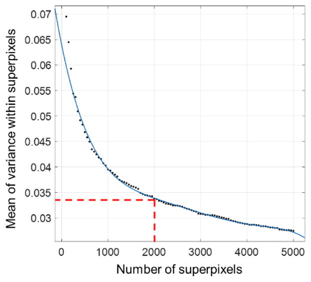
Illustration of mean of gray value variance with different number of superpixels

Since the morphology processing has been utilized to fine tuning the final segmentation result, the effect of the subsequent morphology is investigated. In our experiment, we used opening operation with radius 3 and closing operation with radius 25, both of which is disk-shaped structuring element. We obtained DSC 95.18±1.17 before morphology operation and DSC 97.31±0.36 after morphology operation. The results suggest that the morphology operation only smoothens the edge of segmentation.

Despite the promising results, there are limitations to our study here. First, the available datasets are limited. It is desirable to further validated the algorithm in an independent cohort with more testing cases in the future. Second, several parameters in SBBS-CNN were determined empirically, strategies to auto-determining these parameters would be useful additions to enhance the proposed technique. Finally, due to computation hardware limitation, segmentation in the current work is done in a slice-by-slice fashion with the goal of demonstrating the feasibility and potential benefits of the supervoxel-based approach. The technique can and will be extended to volumetric segmentation in the future. In addition, the correlations among the patches were not considered in the proposed model. A formalism leveraging from inter-supervoxel relationship may further enhance the success of the technique, especially for the segmentation of small sized livers.

5. Conclusion

We proposed SBBS-CNN framework for accurate liver segmentation. In this framework, superpixels are used to facilitate the convolution computation while greatly decreasing the memory usage. Furthermore, a multinomial classification scheme is introduced for the first time to better delineate the liver boundary. It is shown that our method using multinomial SBBS-CNN classification is better than binary classification. The approach is quite general and extendable to other image segmentation problems. Our results show that SBBS-CNN can generate accurate results without any need for complicated postprocessing. Development of a full 3D superpixel-based deep learning that will take full advantage of the rich spatial contextual information is in progress.

References

- Achanta R, Shaji A, Smith K, Lucchi A, Fua P, Süsstrunk S. SLIC superpixels compared to state-of-the-art superpixel methods. IEEE transactions on pattern analysis and machine intelligence. 2012;34:2274–82. doi: 10.1109/TPAMI.2012.120. [DOI] [PubMed] [Google Scholar]
- Bibault J-E, Giraud P, Burgun A. Big data and machine learning in radiation oncology: state of the art and future prospects. Cancer letters. 2016;382:110–7. doi: 10.1016/j.canlet.2016.05.033. [DOI] [PubMed] [Google Scholar]
- Cha KH, Hadjiiski L, Samala RK, Chan HP, Caoili EM, Cohan RH. Urinary bladder segmentation in CT urography using deep-learning convolutional neural network and level sets. Medical physics. 2016;43:1882–96. doi: 10.1118/1.4944498. [DOI] [PMC free article] [PubMed] [Google Scholar]
- Chartrand G, Cresson T, Chav R, Gotra A, Tang A, De Guise JA. Liver Segmentation on CT and MR Using Laplacian Mesh Optimization. IEEE Transactions on Biomedical Engineering. 2016 doi: 10.1109/TBME.2016.2631139. [DOI] [PubMed] [Google Scholar]
- Chen H, Dou Q, Yu L, Qin J, Heng P. NeuroImage. Elsevier; 2017. VoxResNet : Deep voxelwise residual networks for brain segmentation from 3D MR images; pp. 1–10. [DOI] [PubMed] [Google Scholar]
- Dong H, Yang G, Liu F, Mo Y, Guo Y. Automatic Brain Tumor Detection and Segmentation Using U-Net Based Fully Convolutional Networks. Miua. 2017;(1):1–12. doi: 10.1007/978-3-319-60964-5_44. [DOI] [Google Scholar]
- Dou Q, Yu L, Chen H, Jin Y, Yang X, Qin J, Heng P-A. 3D deeply supervised network for automated segmentation of volumetric medical images. Medical Image Analysis. 2017;41:40–54. doi: 10.1016/j.media.2017.05.001. [DOI] [PubMed] [Google Scholar]
- Esteva A, Kuprel B, Novoa RA, Ko J, Swetter SM, Blau HM, Thrun S. Dermatologist-level classification of skin cancer with deep neural networks. Nature. 2017;542:115–8. doi: 10.1038/nature21056. [DOI] [PMC free article] [PubMed] [Google Scholar]
- Ghafoorian M, Karssemeijer N, Heskes T, van Uden IWM, Sanchez C, Litjens IG, de Leeuw F-E, Van Ginneken B, Marchiori E, Platel B. Location Sensitive Deep Convolutional Neural Networks for Segmentation of White Matter Hyperintensities, Scientific Reports. Springer US. 2017;7(1):5110. doi: 10.1038/s41598-017-05300-5. [DOI] [PMC free article] [PubMed] [Google Scholar]
- Google. TensorFlow1.0. 2017 https://www.tensorflow.org/
- Guo Y, Gao Y, Shen D. Deformable MR prostate segmentation via deep feature learning and sparse patch matching. IEEE transactions on medical imaging. 2016;35:1077–89. doi: 10.1109/TMI.2015.2508280. [DOI] [PMC free article] [PubMed] [Google Scholar]
- Han X. Automatic Liver Lesion Segmentation Using A Deep Convolutional Neural Network Method. 2017 doi: 10.1002/mp.12155. https://arxiv.org/pdf/1704.07239v1.pdf. [DOI]
- Hoogi A, Beaulieu CF, Cunha GM, Heba E, Sirlin CB, Napel S, Rubin DL. Adaptive local window for level set segmentation of CT and MRI liver lesions. Medical image analysis. 2017;37:46–55. doi: 10.1016/j.media.2017.01.002. [DOI] [PMC free article] [PubMed] [Google Scholar]
- Hu P, Wu F, Peng J, Liang P, Kong D. Automatic 3D liver segmentation based on deep learning and globally optimized surface evolution. Physics in medicine and biology. 2016;61:8676. doi: 10.1088/1361-6560/61/24/8676. [DOI] [PubMed] [Google Scholar]
- Ibragimov B, Xing L. Segmentation of organs-at-risks in head and neck CT images using convolutional neural networks. Medical Physics. 2017;44:547–57. doi: 10.1002/mp.12045. [DOI] [PMC free article] [PubMed] [Google Scholar]
- Jarrett K, Kavukcuoglu K, LeCun Y. What is the best multi-stage architecture for object recognition? IEEE 12th International Conference on Computer Vision, Kyoto. 2009;2009:2146–2153. [Google Scholar]
- Jirik M, Lukes V, Svobodova M, Zelezny M. Image segmentation in medical imaging via graph-cuts. Computational and Mathematical Methods in Medicine; 11th International Conference on Pattern Recognition and Image Analysis: New Information Technologies (PRIA-11-2013). Samara, Conference Proceedings.2013. [Google Scholar]
- Krizhevsky A, Hinton G. Learning multiple layers of features from tiny images. University of Toronto; 2009. [Google Scholar]
- Krizhevsky A, Sutskever I, Hinton GE. Imagenet classification with deep convolutional neural networks. Proceedings of the 2012 Advances in Neural Information Processing Systems; 2012. pp. 1097–1105. [Google Scholar]
- Li D, Liu L, Chen J, Li H, Yin Y, Ibragimov B, Xing L. Augmenting atlas-based liver segmentation for radiotherapy treatment planning by incorporating image features proximal to the atlas contours. Physics in medicine and biology. 2016;62:272. doi: 10.1088/1361-6560/62/1/272. [DOI] [PMC free article] [PubMed] [Google Scholar]
- Li G, Chen X, Shi F, Zhu W, Tian J, Xiang D. Automatic liver segmentation based on shape constraints and deformable graph cut in CT images. IEEE Transactions on Image Processing. 2015;24:5315–29. doi: 10.1109/TIP.2015.2481326. [DOI] [PubMed] [Google Scholar]
- Litjens G, Kooi T, Bejnordi BE, Setio AAA, Ciompi F, Ghafoorian M, van der Laak JA, van Ginneken B, Sánchez CI. A survey on deep learning in medical image analysis. 2017 doi: 10.1016/j.media.2017.07.005. arXiv preprint arXiv:1702.05747. [DOI] [PubMed] [Google Scholar]
- Long E, Lin H, Liu Z, Wu X, Wang L, Jiang J, An Y, Lin Z, Li X, Chen J. An artificial intelligence platform for the multihospital collaborative management of congenital cataracts. Nature biomedical engineering. 2017;1:0024. [Google Scholar]
- Lu F, Wu F, Hu P, Peng Z, Kong D. Automatic 3D liver location and segmentation via convolutional neural network and graph cut. International journal of computer assisted radiology and surgery. 2017;12:171–82. doi: 10.1007/s11548-016-1467-3. [DOI] [PubMed] [Google Scholar]
- Luo Q, Qin W, Wen T, Gu J, Gaio N, Chen S, Li L, Xie Y. Segmentation of abdomen MR images using kernel graph cuts with shape priors. Biomedical engineering online. 2013;12:124. doi: 10.1186/1475-925X-12-124. [DOI] [PMC free article] [PubMed] [Google Scholar]
- Mharib AM, Ramli AR, Mashohor S, Mahmood RB. Survey on liver CT image segmentation methods. Artificial Intelligence Review. 2012;37(2):83–95. [Google Scholar]
- Milletari F, Navab N, Ahmadi S-A. V-Net: Fully Convolutional Neural Networks for Volumetric Medical Image Segmentation. 2016:1–11. doi: 10.1109/3DV.2016.79. [DOI] [Google Scholar]
- Mylona EA, Savelonas MA, Maroulis D. Entropy-based spatially-varying adjustment of active contour parameters. Image Processing (ICIP), 2012 19th IEEE International Conference on; 2012. pp. 2565–8. [Google Scholar]
- Getreuer Pascal. Chan-Vese Segmentation. Image Processing On Line. 2012;2:214–224. doi: 10.5201/ipol.2012.g-cv. [DOI] [Google Scholar]
- Pawar M, Sale D. MRI and CT Image Denoising using Gaussian Filter, Wavelet Transform and Curvelet Transform. International Journal of Engineering Science and Computing. 2017;7(5):12013–12016. [Google Scholar]
- Pereira S, Pinto A, Alves V, Silva CA. Brain tumor segmentation using convolutional neural networks in MRI images. IEEE transactions on medical imaging. 2016;35:1240–51. doi: 10.1109/TMI.2016.2538465. [DOI] [PubMed] [Google Scholar]
- Ren X, Malik J. Learning a classification model for segmentation, Computer Vision. International Conference on (ICCV); 2003. pp. 10–17. (c) [Google Scholar]
- Ronneberger O, Fischer P, Brox T. U-Net: Convolutional Networks for Biomedical Image Segmentation. International Conference on Medical Image Computing and Computer-Assisted Intervention; 2015; 2015. pp. 234–41. [Google Scholar]
- Roth HR, Farag A, Lu L, Turkbey EB, Summers RM. Deep convolutional networks for pancreas segmentation in CT imaging. 2015 arXiv preprint arXiv:1504.03967. [Google Scholar]
- Shen D, Wu G, Suk H-I. Deep learning in medical image analysis. Annual Review of Biomedical Engineering. 2017;19:221–248. doi: 10.1146/annurev-bioeng-071516-044442. [DOI] [PMC free article] [PubMed] [Google Scholar]
- Tian Z, Liu L, Zhang Z, Fei B. Superpixel-Based Segmentation for 3D Prostate MR Images. IEEE Transactions on Medical Imaging. 2016;35(3):791–801. doi: 10.1109/TMI.2015.2496296. [DOI] [PMC free article] [PubMed] [Google Scholar]
- Wang M, Liu X, Gao Y, Ma X, Soomro NQ. Superpixel segmentation: A benchmark. Signal Processing: Image Communication. 2017;56:28–39. [Google Scholar]
- Wu W, Zhou Z, Wu S, Zhang Y. Automatic liver segmentation on volumetric CT images using supervoxel-based graph cuts. Computational and mathematical methods in medicine. 2016;2016:9093721. doi: 10.1155/2016/9093721. [DOI] [PMC free article] [PubMed] [Google Scholar]
- Yushkevich PA, Piven J, Hazlett HC, Smith RG, Ho S, Gee JC, Gerig G. User-guided 3D active contour segmentation of anatomical structures: Significantly improved efficiency and reliability. NeuroImage. 2006;31(3):1116–1128. doi: 10.1016/j.neuroimage.2006.01.015. [DOI] [PubMed] [Google Scholar]
- Zhang W, Li R, Deng H, Wang L, Lin W, Ji S, Shen D. Deep convolutional neural networks for multi-modality isointense infant brain image segmentation. NeuroImage. 2015;108:214–24. doi: 10.1016/j.neuroimage.2014.12.061. [DOI] [PMC free article] [PubMed] [Google Scholar]
- Zhao X, Wu Y, Song G, Li Z, Fan Y, Zhang Y. Brain Tumor Segmentation Using a Fully Convolutional Neural Network with Conditional Random Fields. International Workshop on Brainlesion: Glioma, Multiple Sclerosis, Stroke and Traumatic Brain Injuries, BrainLes; 2016; 2016. pp. 75–87. Lecture Notes in Computer Science. [Google Scholar]
- Zheng Y, Ai D, Mu J, Cong W, Wang X, Zhao H, Yang J. Automatic liver segmentation based on appearance and context information. Biomedical engineering online. 2017;16:16. doi: 10.1186/s12938-016-0296-5. [DOI] [PMC free article] [PubMed] [Google Scholar]
- Zheng Y, Ai D, Zhang P, Gao Y, Xia L, Du S, Sang X, Yang J. Feature learning based random walk for liver segmentation. PloS one. 2016;11(11):e0164098. doi: 10.1371/journal.pone.0164098. [DOI] [PMC free article] [PubMed] [Google Scholar]