Real-Time Medical Video Denoising with Deep Learning: Application to Angiography

Abstract

This paper describes the design, training, and evaluation of a deep neural network for removing noise from medical fluoroscopy videos. The method described in this work, unlike the current standard techniques for video denoising, is able to deliver a result quickly enough to be used in real-time scenarios. Furthermore, this method is able to produce results of a similar quality to the existing industry-standard denoising techniques.

1. INTRODUCTION

All forms of medical imaging, including computed tomography (CT), magnetic resonance imaging (MRI), plain film x-ray imaging, ultrasound, and optical imaging (for example, endoscopic video), are distorted by noise [1–4].

At the most basic level, noise can be defined as any visual artifact that obscures the features of interest within an image. Such artifacts can appear in many forms, such as graininess, glare, and notching.

1.1 The Impact of Noise in Angiography

Many diagnostic and therapeutic medical interventions rely on live video. Video quality in such interventions is highly important, as the live video is often the primary information source available to the physician during the procedure.

One medical procedure that uses live video is angiography. Angiography is a method of imaging blood vessels. It involves the insertion of a thin metal wire known as a catheter into an artery of the body [5, 6]. A physician guides the catheter through the patient’s blood vessels to a particular target position. Once at the target position, the catheter is used to inject an iodine-rich material into the target vessel. This material shows up well on x-rays, allowing the blood vessels to be imaged (Fig. 1).

Fig 1.

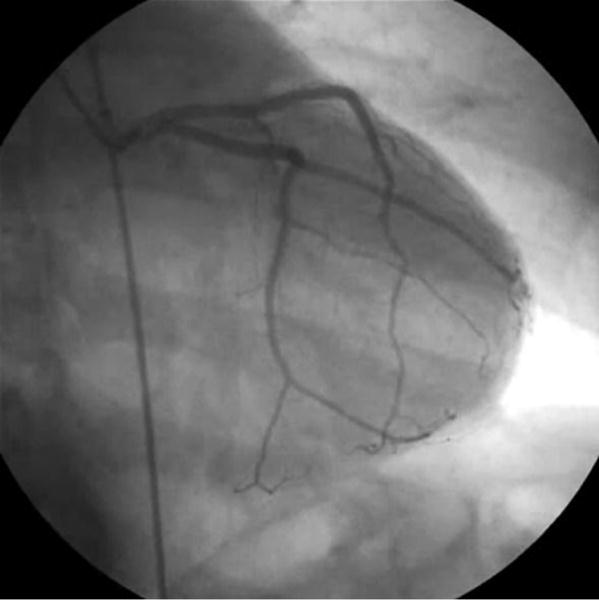
An angiogram of arteries surrounding the heart by Grillo et al. [8], reproduced under the terms of the Creative Commons Attribution 3.0 Unported license.

The catheter can also be used perform a variety of procedures at the target site, including thrombectomy (the removal of a blood clot from a blocked vessel), angioplasty (the use of a small balloon to reopen a blocked artery), or stent placement [6].

When guiding the catheter to the appropriate location, cardiologists rely on real-time x-ray video imaging (known as fluoroscopy) to determine the location of the catheter relative to the patient’s vascular anatomy (Fig. 1). Even with the high quality of modern x-ray instrumentation, interpreting fluoroscopic images during catheter-based procedures can be difficult due to the small size and subtle nature of the vessels on x-ray imaging. Thus, image quality can directly affect the success of such catheter-based procedures.

One of the most common catheter-based procedures is percutaneous coronary intervention, which is the treatment of choice for a patient with an active heart attack [6, 7]. In this procedure, a cardiologist inserts a catheter into the femoral artery in the region of the groin and pushes the catheter upward through the arteries until it reaches the level of the heart. Once there, the catheter is inserted into the coronary arteries—the arteries that directly supply the heart and also the ones that are blocked during a heart attack. The cardiologist uses the catheter to open the blocked blood vessels.

Percutaneous coronary intervention is a technically challenging procedure. Complications resulting from a percutaneous coronary intervention (such as a puncture wound inflicted by the catheter to one of the coronary arteries) require emergency corrective open-heart surgery [6]. In addition, estimates indicate that mortality due to percutaneous coronary intervention may be up to two percent at low-volume centers.

1.2 Denoising Algorithms

Noise is a general problem in imaging that affects not only medicine, but also a wide variety of other fields. There is accordingly a great deal of accumulated research on the subject of computer algorithms for image denoising.

Most approaches to denoising rely on the same fundamental model. Given a true noiseless image $I$, the observer sees a noisy version of that image $I\text{'}$. The noisy image $I\text{'}$ can be defined in terms of the true image $I$:

$$I^{\prime }=f\left(I\right)$$

In this equation, $f$ represents an unknown noise function. The goal of a denoising algorithm, then, is to somehow approximate the noise function $f$ so that the original, noiseless image $I$ can be reconstructed by calculating $f^{-1}\left(I^{\prime }\right)$.

As the number of unknowns is greater than the number of knowns, the problem is underconstrained and any attempts to solve it must therefore rely on assumptions either of the characteristics of the noiseless image $I$ or the noise function $f$.

The current industry-standard denoising algorithm is the block-matching and 3D Filtering (BM3D) algorithm developed by Kostadin et al [9, 10]. BM3D makes assumptions about the structure of the noiseless image $I$: namely that $I$ consists of repeated motifs that are apparent at many parts of the image. The BM3D algorithm aggregates instances of repeated motifs using a block matching technique [11]. An archetypical motif can be computed from the aggregated instances of the motif, and the noise function $f$ can be modeled as a deviation from the motif’s archetype [11].

While BM3D has become the benchmark by which other image denoising algorithms are evaluated, it does have its limitations. Chief among these is speed. BM3D has $O\left(n\right)$ (linear) computational complexity with respect to the number of pixels in the input image but with a high constant factor.

1.3 Deep Learning

In recent years, deep learning has increasingly been applied to medical image analysis problems. Deep learning revolves around the use of artificial neural networks, which are a class of computer algorithms that are loosely modeled on the structure and behavior of biological nervous systems [12]. Just as a biological nervous system is composed of layers of neurons, a neural network is also composed of neuronal layers. Each neuron is connected to neurons within the preceding and successive layers, but not to other neurons within the same layer. The connections are each associated with a numerical weight. As signals propagate down the network, neurons take a weighted sum of the inputs from their upstream connections and apply a mathematical function known as the activation function to determine whether they pass on a signal to downstream neurons and what the magnitude of that signal (if any) should be [12].

Once an annotated dataset is available, a neural network can be trained on that dataset. Training consists of increasing the numerical weights of some inter-neuronal connections and decreasing the numerical weights of other connections until the neural network generates predictions that match the human predictions from the curated training dataset.

Although neural networks have existed for decades, effective algorithms for training them were not available until recently. In particular, neural networks with many layers of neurons—so-called “deep neural networks”—performed poorly when trained with standard techniques.

In 2006, Hinton et al. [13, 14] described a novel method by which deep neural networks could be trained effectively, and subsequent work over the next several years [15, 16] further increased the viability of training deep neural networks for practical applications. This breakthrough led to the development of many specialized sub-types of deep neural networks. Among these specialized subtypes is the convolutional neural network, which is particularly well suited to image analysis problems. Convolutional neural networks have been successfully applied to such diverse tasks as the automatic detection of mitotic cells in histology images [17], of pneumonia in chest X-rays [18], and of diabetic retinopathy in fundoscopic images [19].

There are two key aspects to the function of convolutional neural networks: First, a neuron in the $i$-th layer $L_i$ is not connected to every neuron in the subsequent layer $L_{i+1}$, as it would be in most network architectures. Instead, it is only connected to neurons that encode the information of pixels that are spatially close within the original input image [20]. This gives convolutional networks a tree-like structure (Fig. 2) loosely mirrors the configuration of neurons in the human visual system.

Fig 2.

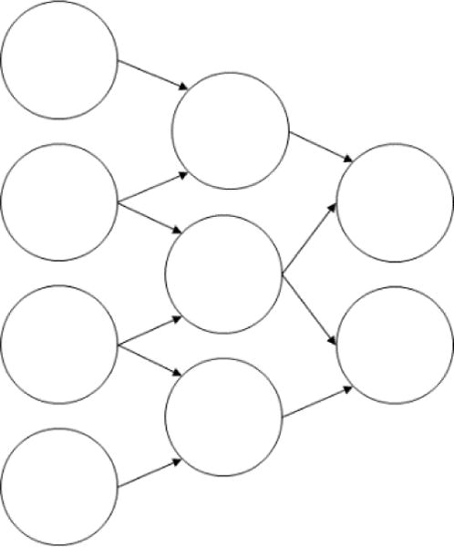
A convolutional neural network

The second key aspect of convolutional neural networks is that they are based on a bank of image processing filters [20]. In a convolutional neural network, the trainable parameters for a particular layer learned numerical entries within a matrix that is used for a filtering operation. By combining many filtering operations, a convolutional neural network can learn from scratch to perform many standard techniques in computerized image analysis, such as blurring, edge detection, and morphologic transformations, as well as more complicated image operations.

Another form of neural network that has become popular in recent years is the autoencoder. Autoencoders are structured such that the number of neurons $N_i$ in the $i$-th layer of a network with $n$ layers satisfies the following relationships:

$$N_1=N_n$$

$$N_i<N_{i-1}\text{ if }i<\frac{n}{2}{N}_i>N_{i-1}\text{ if }i>\frac{n}{2}$$

This structure gives autoencoders a characteristic hourglass appearance (Fig. 3), where the network has a decreasing number of neurons per layer over the first half of the network and an increasing number of neurons per layer over the second half [21].

Fig 3.

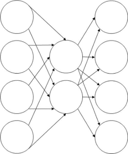
An autoencoding neural network

Autoencoders are trained to maximize the similarity of the outputs to the inputs [21]. Given that intervening layers between the input and output layers have fewer neurons than the input and output layers, this means that the network cannot resort to using a simple identity transformation where the inputs are passed through the network unchanged. Instead, the network must learn a mechanism for converting the inputs to a lower dimensional state and then re-expanding these inputs to the output layer with a minimal loss of information [21]. In other words, autoencoders essentially learn a lossy data compression algorithm for a specific data set with the goal of minimizing the amount of information lost.

An autoencoding neural network architecture can also be useful for learning to normalize or denoise data [22]. This capability stems from the fact that a robust low-dimensional representation of the input to the autoencoder, such as the one encoded in the middle layers of the network, captures stable structures derived from many values or data points [22]. Thus, corruption of a subset of these data points will not affect the learned encoding as long as the degree of corruption remains below a certain threshold.

This work presents a combination of a convolutional neural network architecture with an autoencoding architecture to create a hybrid architecture which is specialized for denoising of image data.

2. METHODS

2.1 Image acquisition and classification

Coronary angiogram videos were acquired from a stock footage vendor. The videos were grayscale with pixel intensities encoded as fractional values between 0.0 and 1.0 has had resolutions ranging from 320 × 240 pixels to 512 × 512 pixels. A total of 20 videos from 20 different procedures were acquired. This data was subjectively divided into “clear” and “noisy” samples, where “clear” videos were those with relatively few noise artifacts and “noisy” videos were those with many. The data was then divided into training and testing sets. Four clear videos were included in the testing dataset. The remaining videos were used as the training dataset.

2.2 Network architecture

A convolutional autoencoding neural network was implemented using the Python programming language and the Keras and TensorFlow toolkits for neural network computations.

The network had thirteen layers:

1. Convolutional layer: 3 × 3 kernel with 70 filters

2. Max pooling layer: stride of two

3. Convolutional layer: 3 × 3 kernel with 60 filters

4. Max pooling later: stride of two

5. Convolutional layer: 3 × 3 kernel with 50 filters

6. Max pooling later: stride of two

7. Convolutional layer: 3 × 3 kernel with 50 filters

8. Upscaling layer: scale factor of two

9. Convolutional layer: 3 × 3 kernel with 60 filters

10. Upscaling layer: scale factor of two

11. Convolutional layer: 3 × 3 kernel with 70 filters

12. Upscaling layer: scale factor of two

13. Convolutional layer: 3 × 3 kernel with one filter

All layers used a rectified linear unit (ReLU) activation function except for the last, which used a sigmoid activation.

2.3 Training

190 still frames were selected out of the set of fluoroscopy videos. These frames came from the “clear” set of videos–they were specifically chosen because they contained little noise. 1,150 patches of 60 × 60 pixels were extracted from the selected still frames at random. These patches were then corrupted with artificial Gaussian noise with a mean of zero and a sigma of 0.05. The corrupted patches were paired with the original, uncorrupted versions of the patches to create the training data set.

The neural network was trained by stochastic gradient decent for 1500 iterations. A mean squared error loss function was used. The learning rate was initially set to 10⁻⁴ and was adjusted as needed during the training process by Adaptive Moment Estimation (commonly known as ADAM optimization).

3. RESULTS

3.1 Gaussian noise

A synthetic evaluation dataset was created in a similar manner to the training dataset. 150 still frames were selected from the set of fluoroscopy videos. These frames came from the “clear” set of videos–they were specifically chosen because they contained little noise.

675 patches of 60 × 60 pixels were extracted from the selected video frames at random. These patches were then corrupted with artificial Gaussian noise with a mean of zero and a sigma of 0.05.

The corrupted patches were fed to the neural network (NN) and the BM3D algorithm to attempt to reconstruct the original, unconstructed patches. The difference between the denoised patch and the original, uncorrupted patch was quantified with mean squared error (MSE) and the structured similarity index (SSIM). Means and standard deviations are reported in Table 1.

Table 1.

Efficacy of Denoising on Gaussian Noise

Method	MSE	SSIM
NN	0.014 ± 0.021	0.99 ± 0.0024
BM3D	1.4×10−4 ± 1.8×10−5	0.97 ± 0.0053

BM3D performs better according to MSE (for which lower values indicate better performance), while the neural network performs better according to SSIM (for which larger values are better). In both cases, the performance difference between the two algorithms is marginal.

Visual inspection of the denoised frames shows that both the BM3D algorithm and the neural network produce images that are highly similar to the original, uncorrupted image (Fig. 5). BM3D tends to produce slightly smoother images with fewer artifacts while the neural network tends to do a better job of preserving very small blood vessels (which tend to be completely eliminated from the denoised images produced by BM3D).

Fig 5.

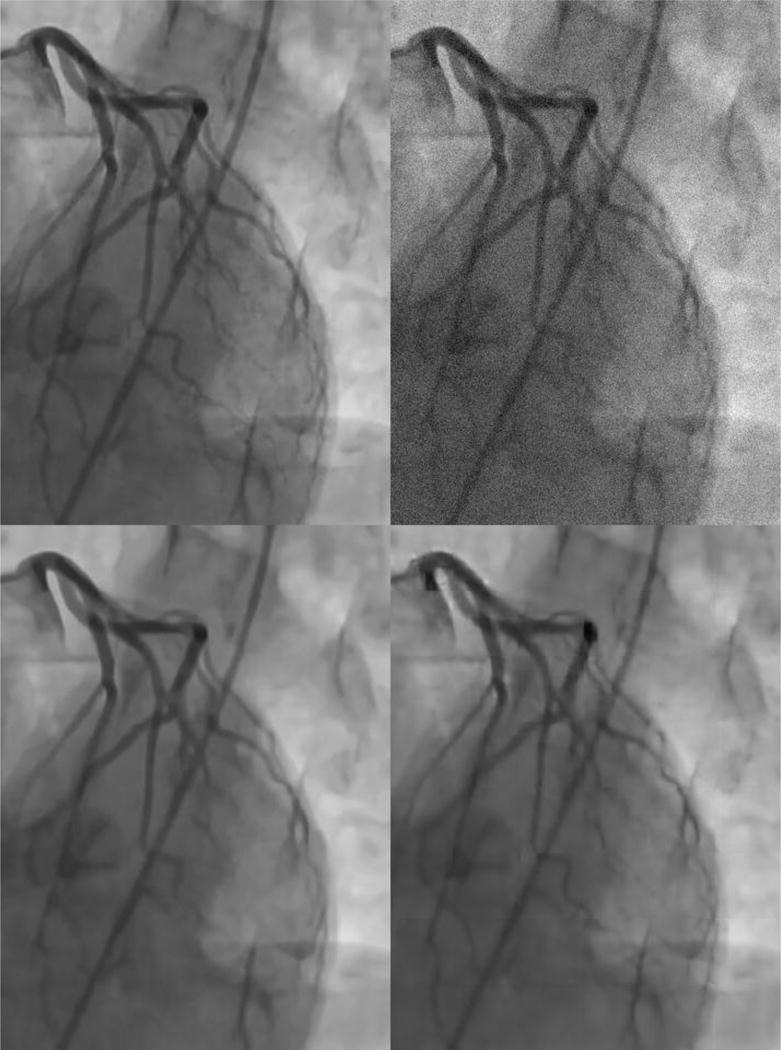
Comparison of denoising algorithms. Clockwise from top left: Original, uncorrupted image; image corrupted with Gaussian noise; denoised image produced by the neural network; denoised image produced by the BM3D algorithm

3.2 Speckle noise

A second evaluation dataset was created. As in the Gaussian noise experiment (Section 3.1), 150 still frames were selected from the set of fluoroscopy videos. These frames came from the “clear” set of videos–they were specifically chosen because they contained little noise.

The chosen images were corrupted with linear multiplicative noise with a mean of zero and a variance of $1/3$. In other words, each pixel $J$ in the corrupted image was a function of the corresponding pixel $I$ in the uncorrupted image as expressed in the following equation:

$$J=I+nI$$

In this equation, $n$ represents a uniformly distributed random variable with a mean of zero and a variance of $1/3$. This form of noise is often referred to as speckle noise.

The corrupted patches were fed to the neural network (NN) and the BM3D algorithm to attempt to reconstruct the original, unconstructed patches. The difference between the denoised patch and the original, uncorrupted patch was quantified with mean squared error (MSE) and the structured similarity index (SSIM). Means and standard deviations are reported in Table 2.

Table 2.

Efficacy of Denoising on Speckle Noise

Method	MSE	SSIM
NN	0.022 ± 0.014	0.99 ± 0.0016
BM3D	9.1×10−4 ± 4.0×10−4	0.88 ± 0.062

It is evident from these results that the BM3D algorithm is less effective at denoising fluoroscopic images when they are corrupted with speckle noise rather than Gaussian noise. The neural network, however, has no drop-off in efficacy when applied to this new form of noise.

3.3 Salt and pepper noise

A third evaluation dataset was created in a similar manner to that of the Gaussian noise dataset (Section 3.1) and the speckle noise dataset (Section 3.2). The images with this dataset were corrupted with a “salt and pepper” strategy: pixels within the image were randomly recolored white or black, each with a probability of 0.05.

The corrupted patches were fed to the neural network (NN) and the BM3D algorithm to attempt to reconstruct the original, unconstructed patches. The difference between the denoised patch and the original, uncorrupted patch was quantified with mean squared error (MSE) and the structured similarity index (SSIM). Means and standard deviations are reported in Table 3.

Table 3.

Efficacy of Denoising on Salt and Pepper Noise

Method	MSE	SSIM
NN	0.19 ± 0.062	0.97 ± 0.0087
BM3D	0.0028 ± 4.3×10−5	0.64 ± 0.037

The BM3D algorithm performed better on the salt and pepper dataset when evaluated by mean squared error, while the neural network performed better as measured by the structured similarity index.

3.4 Speed

100 video frames were selected from the set of fluoroscopy videos at random. 1000 patches were randomly extracted from these videos. Both the neural network and the BM3D algorithms were evaluated on the patches, and the run-times were recoded.

Neural networks are typically executed on graphics processing units (GPUs) as opposed to the central processing unit (CPU). While it is possible in principle to run the BM3D algorithm on a GPU, doing so is rare in practice.

It is important to note that GPUs are known to increase the performance of many image processing tasks by orders of magnitude. Thus, comparing the performance of a neural network on a GPU to the performance of BM3D on a CPU would in essence be a comparison of the processing power of GPUs to CPUs rather than a meaningful comparison of the speeds of the algorithms. To avoid this pitfall, both the neural network and the BM3D algorithm were executed on the CPU for the purposes of the speed comparison. The reference implementation of BM3D created by the original authors of the algorithm [8] was used for this analysis. The results are reported in Table 4.

Table 4.

Denoising Time Per Image on CPU

Method	Time Per Image (seconds)
NN	0.44
BM3D	1.81

As a final test, the neural network was re-executed on a GPU. It took an average of 0.021 seconds to denoise a single image. This is significantly faster than the minimum speed of one frame in 0.33 seconds that is needed to process 30-frame-per-second video in real-time. No third-party GPU-based reference implementation of the BM3D algorithm was available for comparison in this project. However, others have reported a speed up between 2× and 20× with the use of a GPU depending on the size of the input image and the capabilities of the hardware [23]. Upper and lower bound estimates for the performance of BM3D were calculated based on these numbers. These figures are summarized in Table 5.

Table 5.

Denoising Time Per Image on GPU

Method	Time Per Image (seconds)
NN	0.021
BM3D (Low est.)	0.091
BM3D (High est.)	0.910

These numbers show that running the neural network on the GPU would be several times faster than the the BM3D algorithm on the GPU even if it is assumes that the use of a GPU would provide a 20× speedup, which is the highest figure that has been reported in the literature [23].

4. CONCLUSION

This results in this article show that a deep learned approach to video denoising can produce results of similar quality to BM3D, the current industry-standard algorithm for denoising. Furthermore, the results in this article show that deep learned video denoising can be significantly faster than BM3D and is fast enough to process video in real-time.

The deep learned algorithm, which was trained exclusively on examples of images that were corrupted with Gaussian noise, was able not only to match the efficacy of BM3D in removing Gaussian noise, but also to meet or exceed the efficacy of BM3D in removing speckle noise and salt and pepper noise. Deep learning is therefore a particularly versatile method for denoising medical angiograms.

Angiography is one of a wide variety of modern medical procedures and interventions rely on high quality video for guidance and decision making. Given the importance of video as an information source during such procedures, there is good reason to believe that improving the quality and thus interoperability of the video can directly lead to beneficial effects in terms of procedure time and outcomes.

The neural network model makes a tradeoff between performance and generality. As the neural network presented in this article was trained exclusively on fluoroscopic x-ray images, it has no knowledge of the specific features found within other types of images, such as x-rays that show bones instead of blood vessels, or ultrasound images as opposed x-ray images, or images of a completely nonmedical subject matter. It is therefore unlikely to transfer well to these types of images. The BM3D algorithm, in contrast, does not rely on knowledge of the particular subject matter of the image.

Thus far in this article, two classes of artificial neural networks have been discussed: convolutional neural networks and autoencoding neural networks. Neither of these forms of neural network has a native mechanism for representing time series data. In other words, they process video data as a bag of unrelated still image video frames. Any relationships between video frames that are temporally close are ignored. There is a third form of neural network that does have a native mechanism for modeling time series relationships: the recurrent neural network [24]. Recurrent neural networks have been used primarily for the analysis of textual data but have also seen some use in image analysis contexts [24].

A hybrid architecture that blends the properties of a recurrent neural network with the convolutional autoencoding architecture described in this article could leverage the temporal aspect of video and potentially yield denoised images of higher quality or yield images of similar quality, but with fewer neurons and thus fewer parameters to train. The authors plan to investigate the potential of incorporating aspects of recurrent neural networks into video denoising in future work.

Fig 4.

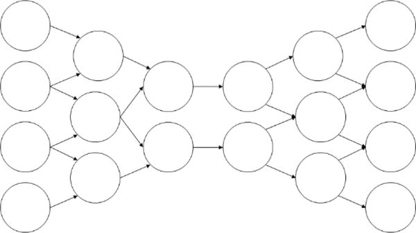
A combined convolutional/autoencoding neural network architecture

References

- 1.Borsdorf A, Raupach R, Flohr T, Hornegger J. Wavelet Based Noise Reduction in CT Images Using Correlation Analysis. IEEE Transactions on Medical Imaging. 2008 Dec;27:1685–1703. doi: 10.1109/TMI.2008.923983. 2008. [DOI] [PubMed] [Google Scholar]
- 2.Macovski A. Noise in MRI. Magnetic Resonance in Medicine. 1996 Sep;36:494–497. doi: 10.1002/mrm.1910360327. 1996. [DOI] [PubMed] [Google Scholar]
- 3.Mateo JL, Fernández-Caballero A. Finding out general tendencies in speckle noise reduction in ultrasound images. Expert Systems with Applications. 2009 May;36:7786–7797. 2009. [Google Scholar]
- 4.Zhang C, Helferty JP, McLennan G, Higgins WE. Nonlinear distortion correction in endoscopic video images. Proceedings of the 2000 International Conference on Image Processing. 2003 Sep;:3. 2000. [Google Scholar]
- 5.Jolly SS, Amlani S, Hamon M, Yusuf S, Mehta SR. Radial versus femoral access for coronary angiography or intervention and the impact on major bleeding and ischemic events: A systematic review and meta-analysis of randomized trials. American Heart Journal. 2009 Jan;157:123–140. doi: 10.1016/j.ahj.2008.08.023. 2009. [DOI] [PubMed] [Google Scholar]
- 6.Patel VG, Brayton KM, Tamayo M, Mogabgab O, Michael TT, Lo N, et al. Angiographic Success and Procedural Complications in Patients Undergoing Percutaneous Coronary Chronic Total Occlusion Interventions: A Weighted Meta-Analysis of 18,061 Patients From 65 Studies. JACC Cardiovascular Intervention. 2013 Feb;6:128–138. doi: 10.1016/j.jcin.2012.10.011. 2013. [DOI] [PubMed] [Google Scholar]
- 7.Godino C, Colombo A. Complications of Percutaneous Coronary Intervention. PanVascular Medicine. 2015 Feb;:2297–2322. 2015. [Google Scholar]
- 8.Grillo T, Athayde G, Belfort A, Miranda R, Beaton A, Nascimento B. Mitral Subvalvular Aneurysm in a Patient with Chagas Disease and Recurrent Episodes of Ventricular Tachycardia. Case Reports in Cardiology. 2015 Nov; doi: 10.1155/2015/213104. 2015. [DOI] [PMC free article] [PubMed] [Google Scholar]
- 9.Kostadin D, Foi A, Katkovnik V, Egiazarian K. Image denoising by sparse 3-D transform-domain collaborative filtering. IEEE Transactions on Image Processing. 2007 Jul;16:2080–2090. doi: 10.1109/tip.2007.901238. 2007. [DOI] [PubMed] [Google Scholar]
- 10.Shao L, Yan R, Li X, L Y. From Heuristic Optimization to Dictionary Learning: A Review and Comprehensive Comparison of Image Denoising Algorithms. 2013 Aug;44:1001–1013. doi: 10.1109/TCYB.2013.2278548. 2013. [DOI] [PubMed] [Google Scholar]
- 11.Hasan MM. Thesis. University of Western Ontario; May, 2014. Adaptive Edge-guided Block-matching and 3D filtering (BM3D) Image Denoising Algorithm. 2014. [Google Scholar]
- 12.LeCun Y, Bengio Y, Hinton GE. Deep learning. Nature. 2015 May;521:436–444. doi: 10.1038/nature14539. 2015. [DOI] [PubMed] [Google Scholar]
- 13.Hinton GE, Osindero S, Teh YW. A Fast Learning Algorithm for Deep Belief Nets. Neural Computation. 2006 Jul;18:1527–1554. doi: 10.1162/neco.2006.18.7.1527. 2006. [DOI] [PubMed] [Google Scholar]
- 14.Hinton GE. Learning Multiple Layers of Representation. Trends in Cognitive Sciences. 2007 Oct;11:428–434. doi: 10.1016/j.tics.2007.09.004. 2007. [DOI] [PubMed] [Google Scholar]
- 15.Deng L, Li J, Huang JT, Yao K, Yu D, Seide F, et al. Recent Advances in Deep Learning for Speech Research at Microsoft. Proceedings of the 2013 IEEE Conference on Acoustics, Speech and Signal Processing (ICASSP) 2014 May;:8604–8608. 2013. [Google Scholar]
- 16.Hinton GE, Deng L, Yu D, Dahl GE, Mohamed A, Jaitly N, et al. Deep Neural Networks for Acoustic Modeling in Speech Recognition: The Shared Views of Four Research Groups. IEEE Signal Processing. 2012 Jul;29:82–97. 2012. [Google Scholar]
- 17.Cireşan DC, Giusti A, Gambardella LM, Schmidhuber J. Mitosis Detection in Breast Cancer Histology Images with Deep Neural Networks. Medical Image Computing and Computer-Assisted Intervention. 2013 Oct;:16–2. 411–418. doi: 10.1007/978-3-642-40763-5_51. 2013. [DOI] [PubMed] [Google Scholar]
- 18.Rajpurkar P, Irvin J, Zhu K, Yang B, Mehta H, Duan T, et al. CheXNet: Radiologist-Level Pneumonia Detection on Chest X-Rays with Deep Learning. arXiv preprint (arXiv:171105225 2017) 2017 [Google Scholar]
- 19.Abràmoff MD, Lou Y, Erginay A, Clarida W, Amelon R, Folk JC, et al. Improved Automated Detection of Diabetic Retinopathy on a Publicly Available Dataset Through Integration of Deep Learning. Investigative Ophthalmology & Visual Science. 2016 Oct;13:5200. doi: 10.1167/iovs.16-19964. 2016. [DOI] [PubMed] [Google Scholar]
- 20.Krizhevsky A, Sutskever A, Hinton GE. Advances in Neural Information Processing Systems. Vol. 25. NIPS; 2012. Imagenet classification with deep convolutional neural networks. 2012. [Google Scholar]
- 21.Hinton GE, Salakhutdinov RR. Reducing the dimensionality of data with neural networks. Science. 2006 Jul;313:504–507. doi: 10.1126/science.1127647. 2006. [DOI] [PubMed] [Google Scholar]
- 22.Vincent P, Larochelle H, Bengio Y, Pierre-Antoine M. Extracting and composing robust features with denoising autoencoders. Proceedings of the 25th International Conference on Machine Learning. 2008 Jul;25:1096–1103. 2008. [Google Scholar]
- 23.Honzátko D, Kruliš M. Accelerating block-matching and 3D filtering method for image denoising on GPUs. Journal of Real-Time Processing. 2017 Nov;37:1–15. 2017. [Google Scholar]
- 24.Mikolov T, Karafiát M, Burget L, Černocký J, Khudanpur S. Recurrent neural network based language model. 11th Annual Conference of the International Speech Communication Association. 2010 Sep;11:1045–1048. 2010. [Google Scholar]