Automatic Recognition of Holistic Functional Brain Networks Using Iteratively Optimized Convolutional Neural Networks (IO-CNN) with Weak Label Initialization

Abstract

fMRI data decomposition techniques have advanced significantly from shallow models such as Independent Component Analysis (ICA) and Sparse Coding and Dictionary Learning (SCDL) to deep learning models such Deep Belief Networks (DBN) and Convolutional Autoencoder (DCAE). However, interpretations of those decomposed networks are still open questions due to the lack of functional brain atlases, no correspondence across decomposed or reconstructed networks across different subjects, and significant individual variabilities. Recent studies showed that deep learning, especially deep convolutional neural networks (CNN), has extraordinary ability of accommodating spatial object patterns, e.g., our recent works using 3D CNN for fMRI-derived network classifications achieved high accuracy with a remarkable tolerance for mistakenly labeled training brain networks. However, the training data preparation is one of the biggest obstacles in these supervised deep learning models for functional brain network map recognitions, since manual labelling requires tedious and time-consuming labors which will sometimes even introduce label mistakes. Especially for mapping functional networks in large scale datasets such as hundreds of thousands of brain networks used in this paper, the manual labelling method will become almost infeasible. In response, in this work, we tackled both the network recognition and training data labelling tasks by proposing a new iteratively optimized deep learning CNN (IO-CNN) framework with an automatic weak label initialization, which enables the functional brain networks recognition task to a fully automatic large-scale classification procedure. Our extensive experiments based on ABIDE-II 1,099 brains’ fMRI data showed the great promise of our IO-CNN framework.

1. INTRODUCTION

Reconstructing concurrent functional brain networks from fMRI blood oxygen level dependent (BOLD) data has been investigated for decades. The reconstructed concurrent functional brain networks help us better understand functional human brain activities and their underlying neural substrates. Traditionally, independent component analysis (ICA) (Cole et al., 2010; McKeown et al., 2003) and general linear model (GLM) (s et al., 1994a; Logothetis, 2008) have been widely utilized for resting state functional networks and task-evoked functional networks, respectively. Typically, the number of network components that can be reconstructed from ICA or GLM method is up to several dozens, which are defined by the number of brain sources (Cole et al., 2010) for ICA and the number of linear compounds of parameter estimates (COPE) (Friston et al., 1994) for GLM. In recent several years, a new computational framework of sparse representation (Lv et al., 2015a, 2015b; Mairal et al., 2010) of whole-brain fMRI signals was proposed and used for both resting state and task-evoked fMRI signal decompositions. Typically, hundreds of concurrent functional networks can be reconstructed effectively and robustly by sparse representation methods, thus forming holistic atlases of functional networks and interactions (HAFNI) (Lv et al., 2015b). Concurrent functional networks decomposed by this method have been shown to be superior in revealing the reconstructed task-evoked and/or resting state networks’ spatial overlaps and their corresponding functions (Lv et al., 2015b).

Recently, deep learning has attracted much attention in the field of machine learning and data mining (Bengio et al., 2013), and deep learning approach is proven to be superb at learning high-level and mid-level features from low-level raw data (Schmidhuber, 2014). A deep learning architecture usually consists of several numbers of layers by stacking multiple similar building blocks. The top layer receives an input and then passes the extracted features of the input to the next layer, all the way down from the top layer to the bottom layer. As a result, the architecture of a deep learning model acts as a hierarchical feature extractor at different levels. Instead of using abovementioned shallow models to reconstruct functional brain networks, some novel deep models have been explored recently. For instance, Restricted Boltzmann Machine (RBM) and deep convolutional autoencoder (DCAE) have both been leveraged for applications in fMRI signal analysis and modeling (Han et al., 2015; Huang et al., 2017; Zhao et al., 2017a). New methodologies are still emerging for reconstructing brain networks to offer the fundamental understanding of functional brain mechanisms.

With the availability of such well reconstructed functional brain networks across different individual brains using the abovementioned methods, the next step would be to model, interpret and use them in a neuroscientific meaningful context. However, due to the random initialization nature of the decomposition algorithms in ICA, sparse representation or other methods, together with the variability and heterogeneous characteristics of human brains, the correspondences of the decomposed networks across different brains are not established nor guaranteed, which results in the problems for group level modeling and statistically meaningful analysis for the obtained networks (Lv et al., 2013; Smith et al., 2009; Y. Zhao et al., 2016). Previously, group-wise functional network decomposition techniques were utilized for extracting networks that are consistent across subjects in a group level (Lv et al., 2015c, 2013; S. Zhao et al., 2016). For instance, in the HAFNI system, 23 task-evoked and 10 resting state group-wise consistent networks were identified and confirmed as functional atlases. This approach works decently on small scale of fMRI data, but it is not able to scale up to large scale datasets and cannot deal with the inevitable individual heterogeneity. Another study by our research group attempted to accurately and effectively integrate group-wisely consistent spatial networks decomposed at individual level by using spatial overlap rate similarity assisted by a spatial map descriptor called connectivity map (Y. Zhao et al., 2016), in which 144 functional atlases were generated across populations. Though the connectivity map model has achieved promising results (Y. Zhao et al., 2016), it is still noticeable that dealing with the tremendous variability of various types of functional brain networks and the presence of various sources of noises is still very challenging, due to the limited ability of the model itself to describe various spatial pattern distributions.

So far, the lack of effective spatial volume map descriptors has been realized as a major challenge for all functional networks analysis related research studies, such as integrating networks atlases and functional network recognition tasks. In the natural image classification and recognition field, e.g., ImageNet challenge (Jia Deng et al., 2009), a specific type of deep learning networks, convolutional neural networks (CNNs), has shown the extraordinary ability in accommodating spatial object pattern representations (He et al., 2015; Karpathy et al., 2014; Krizhevsky et al., 2012; Lawrence et al., 1997; Lecun et al., 1998; Nian Liu et al., 2015; Simonyan and Zisserman, 2014). In the context of this paper, the lack of functional brain atlases and no correspondence across decomposed or reconstructed networks across different subjects are considered as a big challenge for brain network classification and recognition. Furthermore, the significant individual variabilities in functional brain networks made it even more challenging. Faced with these challenges and inspired by all those great accomplishments achieved by using deep learning (especially CNN for spatial pattern description), in our previous work (Zhao et al., 2017b), an effective 3D CNN framework was designed and applied to achieve effective and robust functional network identification by both accommodating manual label mistakes and outperforming traditional spatial overlap rate based methods.

However, even though our 3D CNN model with two convolutional layers, one pooling layer and two fully connected layers for functional network map recognition has successfully achieved high accuracy in functional networks recognition, the classification category number is only limited to 10 most common networks. More importantly, around 5,000 training networks preparation went through a very tedious inter-expert manual label work procedure over 210,000 functional networks. As indicated in (Zhao et al., 2017b), due to the highly interdigitated and spatially overlapped nature of the functional brain organization (Xu et al., 2016), the manual labelling process will inevitably introduce some mistakes into the training set labels. As model goes deeper and deeper, sufficient amount of data is needed for training the model (LeCun et al., 2015). As a result, the accurate labelling and the fast labelling process become the major need for training a deep learning model of functional brain networks.

In response to address the abovementioned large-scale training data preparation problem and extend the previous 10-class CNN-based recognition to large-scale functional network recognition, a novel iteratively optimized CNN (IO-CNN) framework is proposed here, while the initialization network labels were roughly assigned using automatic overlap rate based label. The training dataset is based on 219,800 functional networks decomposed from 1099 subjects’ fMRI data provided by publicly available database ABIDE II (http://fcon_1000.projects.nitrc.org/indi/abide/abide_II.html). After training, an accurate functional network recognition and identification based on the IO-CNN for 135 functional network atlases will be achieved. Extensive experiments on the ABIDE-II 1,099 brains’ fMRI data has demonstrated that the proposed IO-CNN framework has superior spatial pattern modelling capability in dealing with various types of network maps, and the iterative optimization algorithm can gradually accommodate the mistaken labels introduced by the fully automatic but rough label initialization, eventually converging to a fine-grained classification accuracy. In general, the automatic rough label initialization together with the iterative optimization framework provides novel and deep insight in training and applying large scale deep learning networks with weak label supervision, contributing to the general field of deep learning for medical imaging.

2. METHODS AND MATERIALS

2.1 Dataset and preprocessing

Our experimental data were downloaded from the publicly available Autism Brain Imaging Data Exchange II (ABIDE II: http://fcon_1000.projects.nitrc.org/indi/abide/abide_II.html). The ABIDE was established for discovery science on the brain connectome in autism spectrum disorder (ASD). ABIDE I already demonstrated the feasibility and utility of aggregating fMRI data across different sites, while ABIDE II was promoted further for that purpose with larger scale of datasets. To date, ABIDE II involves data from 19 sites with 521 ASD patients and 593 controls (5–64 years old). After manually checking data quality according to preprocessing (e.g. skull removal, registration to standard space) results, only 511 ASD patients and 588 control subjects are selected, which were then used in our following experiments. The acquisition parameters vary across different sites: 190 – 256 mm FOV, 31 – 50 slices, 0.475 – 5.4 s TR, 24 – 86 ms TE, 60 – 90 ° flip angle, (2.5 – 3.8) × (2.5 – 3.8) × (2.5 – 4) mm voxel size. For detailed parameters for each site, please refer to the ABIDE II website.

Preprocessing for the resting state fMRI (rsfMRI) data were performed using the FSL software tools (Jenkinson et al., 2012), including skull removal, motion correction, spatial smoothing, temporal pre-whitening, slice time correction, global drift removal, and linear registration to the Montreal Neurological Institute (MNI) standard brain template space, which were all implemented by the FSL FLIRT and FEAT commands.

After preprocessing, we exploited dictionary learning and sparse coding techniques (Lv et al., 2015a, 2015b) for functional brain networks reconstruction for each subject. The input for dictionary learning is a matrix X ∈ ℜ^t×n with t (length of time points) rows by n columns containing normalized (normalizing signals to 0 mean and standard deviation of 1) fMRI signals from n brain voxels of an individual subject. The output contains one learned dictionary D and a sparse coefficient matrix α ∈ ℜ^m×n, w.r.t, X = D × α + ε, where ε is the error term and m is the predefined dictionary size. Each row of the output coefficient matrix α was then mapped back to the brain volume space as a 3D spatial map of functional brain network. According to (Lv et al., 2015a; Y. Zhao et al., 2016), dictionary size m was empirically set to 200 for a comprehensive functional brain networks reconstruction, which means each individual fMRI data will have 200 decomposed functional networks.

2.2 3D CNN Model

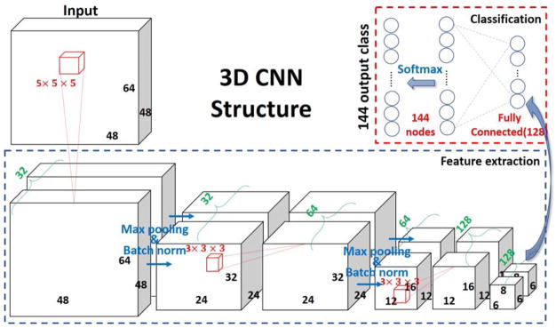
As demonstrated in (Zhao et al., 2017b), 3D convolutional neural network (CNN) has promising performance in modeling 3D spatial distribution patterns and correcting outliers by modeling each class’s spatial distribution, especially for functional brain maps. Thus, in this work, we adopted and modified the previous CNN structure (Zhao et al., 2017b) to a new 3D CNN net (shown in Fig. 1) with 3 convolutional blocks for feature extraction, and two fully connected layers for classification. Specifically, each convolutional block contains 3 layers: 1) convolutional layer with rectified nonlinearity unit (ReLU) as activation function (Maas et al., 2013), which is not shown in Fig. 1 for brevity. The initialization scheme of the convolutional layers was adopted from the methods in (He et al., 2015); 2) A pooling layer is connected to the convolutional layers. This layer reduces redundant input information and introduces translation-invariance characteristics (Scherer et al., 2010), which is aimed to alleviate the possible global shift resulted by image registration and the intrinsic variability of different individual brains. In this paper, a max pooling scheme with a pooling size of 2 was adopted and it turned out to work quite well (Zhao et al., 2017b); 3) Batch normalization layer is introduced later to enable faster learning and remove internal covariate shift of each mini-batch (Ioffe and Szegedy, 2015).

Fig. 1.

3D CNN structure used for training and classification. Bold numbers indicated the feature map sizes (e.g. 48, 64, 48); Red numbers indicated convolutional kernel size (e.g. 3 × 3 × 3) and nodes number of fully connected layers (e.g. 128, 144); Green numbers indicated the channel size of each feature map.

The feature extraction part will be accomplished by the 3 convolutional blocks and herein comes with the following fully connected layers for classification purpose. As illustrated in Fig. 1, only one hidden layer with 128 nodes were inserted between the output nodes and the extracted feature maps from the convolutional blocks. A softmax function is then applied to obtain the probability of the final predictions.

The loss function used for this canonical multi-class classification problem is the categorical cross entropy (1).

$$L(\theta )=-\frac{1}{n}{\sum }_{i=1}^n{\sum }_{j=1}^{k}1\{y^i=j\}log{\left({\theta }^T{x}^i\right)}_j$$ (1)

where n is the number of samples in one batch (empirically set to 20), k is the number of the output classes (144 output classes), and log(θ^T xⁱ)_j is the log-likelihood activation value of the j_th output node. The optimizer used for the backpropagation is the advanced ADADELTA (Zeiler, 2012). θ is the network structure weights matrix. yⁱ is the training label.

As the input volumes have dimensions of 48 × 64 × 48 and the full volume with a batch size of 20 was used, 4.2GB memory will be consumed on the GPU card for training the proposed 3D CNN model.

2.3 Iteratively Optimized CNN (IO-CNN) with weakly label initialization

Unlike the previous project, we do not simply train the inherited and improved CNN mentioned in section B using the same training dataset. Instead, we proposed a new Iteratively Optimized CNN (IO-CNN) to iteratively train on dynamically updated training sets. Specifically, the initial training dataset is generated using a fast and automatic, but weak, labelling process by utilizing the maximal spatial overlap rate scheme, as mentioned in (Zhao et al., 2017b). Notably, this automatic labelling scheme can still achieve around 85% accuracy on prediction, providing a rough but fairly good enough training initialization.

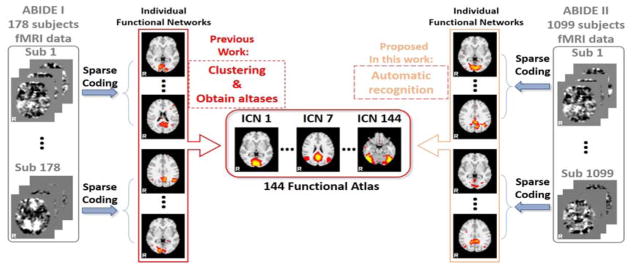
The classification labels are the 144 functional network atlases generated in (Y. Zhao et al., 2016), by using the ASD and Typical Control (TC) populations (from ABIDE I dataset). After performing sparse coding on each subject’s fMRI data, we obtained 200 functional network components for each subject. Then the labelling scheme for each component is to assign the label of the template with maximum overlap rate among the 144, as long as the maximum overlap rate is larger than 0.2. Otherwise, that component will be assigned with label 0 (Table I). Briefly, the 144 functional network atlases are generated from the ABIDE I dataset by utilizing a clustering scheme based on spatial overlap rate metrics, which are assisted and accelerated by the proposed connectivity map in (Y. Zhao et al., 2016). Based on the 144 functional network atlases as classification labels, the larger scale dataset of ABIDE II was then used for the recognition and identification tasks. Fig. 2 described the logic relationship and connection between our previous work of generating 144 functional atlases from ABIDE I data in (Y. Zhao et al., 2016) and current work of weakly labeling the reconstructed functional networks from ABIDE II data.

Table I.

Algorithm for IO-CNN

Algorithm: deep iterative CNN with week label initialization
Input: 1). 219,800 individual functional networks (1099 subjects, with 200 functional network each); 2). 144 functional atlases
Initialization: 1). Calculate pairwise overlap rate between individual functional networks and functional atlases → 219,800 × 144 similarity matrix S0
2). Threshold overlap rate value in S below 0.2 to be 0;
3). For each individual network row ${\mathit{S}}_i^0$ in S0do
If ${\mathit{S}}_i^0=\mathbf{0}$ then
labeli = 0
Else
${\mathit{label}}_i=\mathit{argmax}({\mathit{S}}_i^0)$
$\{\mathit{argmax}({\mathit{S}}_i^0)\in \mathit{N}\mid 1\le \mathit{argmax}({\mathit{S}}_i^0)\le 144\}$
End
End
Return label0
Deep iterative training: using none zero labeled individual functional networks and label0a as initial training pairs.
For i in {0, 1, 2, …, maxIter} do
Train CNN on
[none zero labeled individual functional networks, labeli]
labeli+1 = CNNmodel predict on
all functional networks,
label_diff = diff (labeli, labeli+1)
If | label_diff|/219, 800 < 0.4%
Break
End
End
Return CNNmodel

Fig. 2.

Logic connection between the atlases generation based on ABIDE I data in (Y. Zhao et al., 2016) and the functional network recognition work based on these atlases using the ABIDE II data in this paper. Both ADIBE I and II fMRI datasets were decomposed to functional networks using sparse coding, where networks from ABIDE I were utilized for generating atlases, while the functional networks from ABIDE II were decomposed for atlases-based recognition via a weak labeling process based on spatial overlap rate.

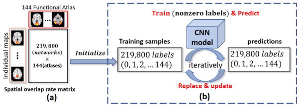
Based on the 144 functional atlases from ABIDE I dataset and the individual functional networks derived from ABIDE II dataset, the initial network labels were automatically and roughly assigned to each of the 219,800 networks by calculating the spatial overlap rate similarity matrix as shown in (a). The spatial overlap rate is calculated in (2):

$$\text{overlap}\text{rate}={\sum }_{k=1}^{\mid V\mid }\frac{min(V_k,W_k)}{(V_k+W_k)/2}$$ (2)

where V_k and W_k are the activation scores of voxel k in network volume maps V and W, respectively. To ensure the accuracy of the initial label assigned by this method, the empirical thresholding (threshold 0.2) process was applied on the similarity matrix, as demonstrated in (Y. Zhao et al., 2016). For each individual network map, the label is assigned as atlas number whose spatial overlap rate is the maximum among all 144 atlases. In the case of no similarity value is above 0.2, the corresponding network map will be assigned the label 0, which will not be used in training the 3D CNN. The IO-CNN training process will begin after label initialization (a).

The detailed algorithm part of IO-CNN() is elaborated in Table I. Briefly, the IO-CNN training process will iterate over the 219,800 input 3D network maps for a maximum N (e.g., N=20) iterations, starting with the initial weak labels based on spatial overlap rate. As mentioned in (Zhao et al., 2017b), spatial overlap based classification can achieve around 85% accuracy on prediction, while the CNN scheme has the superior ability for label correction on that prediction, thus improving the recognition accuracy. This intriguing label correction capability is adopted in the IO-CNN framework to improve the previously assigned training labels during each iteration, thus introducing changes between the labels predictions after training and the labels before training. This improvement is a core methodological contribution of this paper, in addition to the dramatically increased number of used subjects (1,099 subjects in total) and the much larger number of network labels (144 as an initialization). After iterative optimization, a balance will be achieved by the IO-CNN framework when no significant changes (e.g., less than 0.5%) occurs, thus yielding the optimized and well-trained CNN model for functional brain network recognition.

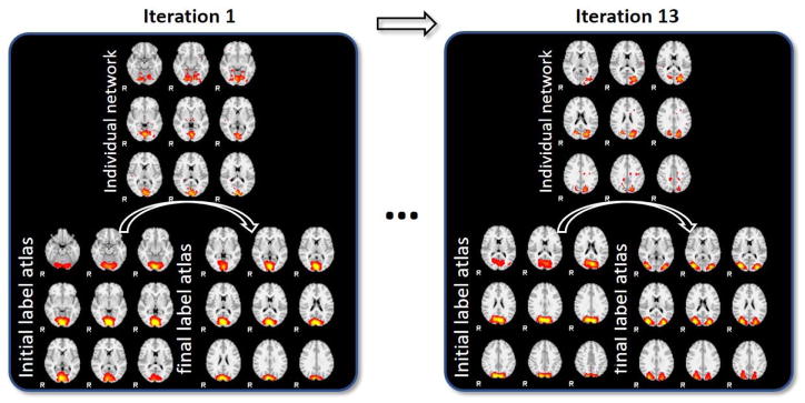
Specifically, the maxIter is set to 20 in case of stopping loop for oscillation, and the number of training epoch for each CNN training is empirically set to 5. The actual stop condition is reached at iteration 13, during which the label change procedure is illustrated in Fig. 4 as an example.

Fig. 4.

Label change procedure during each iteration. During each iteration, initially assigned labels of some networks will be optimized to other labels during the CNN training iteration.

3. RESULTS

3.1 IO-CNN Training Details

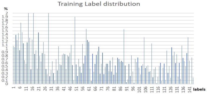
As we have introduced before, the training dataset is based on the decomposed functional networks using dictionary learning and sparse coding methods from ABIDE II dataset. After the rough label initialization process proposed in Table I as the first step, the label distribution for 144 functional network atlases consisting of 80,293 training samples are shown in Fig. 5. As we can see, most of training samples have relatively balanced labels except for a few (9 labels) labels whose training sets only have less than 0.15% samples. This is probably due to the imperfectness of the functional network atlases generated in our previous work (Y. Zhao et al., 2016), in that atlases with only minor individual networks among the population will not be regarded as intrinsic functional networks (Fox et al., 2005). As the IO-CNN training iteration goes on, the minor atlas training samples will be eliminated or moved to other atlas labels, which reaches a final label number of 135 after the IO-CNN training converges.

Fig. 5.

Initial training set’s 144 functional network label distributions.

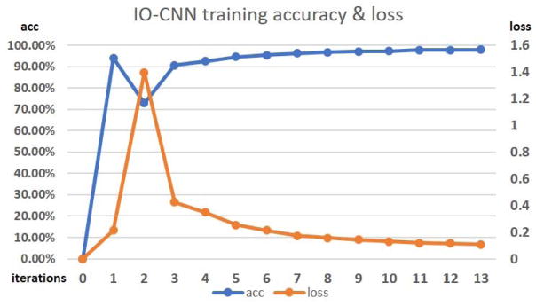
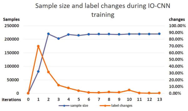
The training gradually converges to an optimization point as the iteration number increases, as shown in Fig. 6. Clearly, we can see that there is a significant accuracy drop during iteration 2, which is probably caused by the significant increase in training sample size from the initial training sample size of 80,293 to the size of 219,787 (Fig. 7). Then, the training sample size remains relatively stable, thus following a stable increasing training accuracy and decreasing loss. The convergence is reached at iteration 13, where the training sample label change over the previous iteration is less than 0.4%, which indicates the optimization of the IO-CNN, thus terminating the training iterations.

Fig. 6.

IO-CNN training accuracy and loss curves from iteration 0 to 13. Iteration 0 is the weak label initialization process, where IO-CNN is not trained yet.

Fig. 7.

Sample size’s dynamic changes and label change percentages during IO-CNN training. Iteration 0 is the weak label initialization process, where IO-CNN is not trained yet. Initial labels (80,293 initial training samples) were first used in iteration 1 for IO-CNN training.

For our IO-CNN training, Keras (https://keras.io/) framework with tensorflow (https://tensorflow.org) backend on an 8 GB memory GPU (Nvidia Quadro M4000) was utilized. The training time for each iteration is also dependent on the training sample size (average training samples size is 206,524 per iteration). A total time of 3.8 days (91 hours) was spent for all the 13 iterations of IO-CNN training (7 hours per iteration).

3.2 Recognition Results

The optimized IO-CNN model shows 87.5% prediction consistency with the initial overlap based training label, which is consistent with the overlap based recognition accuracy of 85.93% reported in our previous work (Zhao et al., 2017b), further demonstrating the deficiency in functional network recognition task using spatial overlap based methods. It is worth noting that functional network spatial overlap is a natural property of functional organization of the human brain (Xu et al., 2016), in that cortical microcircuits overlap and interdigitate with each other (Harris and Mrsic-Flogel, 2013), rather than being independent and segregated in space. Thus, it is critically important to develop novel and effective methods to recognize spatially overlapping functional networks. In this paper, the network recognition and classification are based on the previously generated 144 atlases, which can be found and visualized at http://hafni.cs.uga.edu/autism/templates/all.html. As we can see, some of the 144 network atlases are highly spatially overlapped but they remain functionally distinct, e.g., Fig. 4 shows that the final label atlas and initial label atlas are quite similar due to the high spatial overlap.

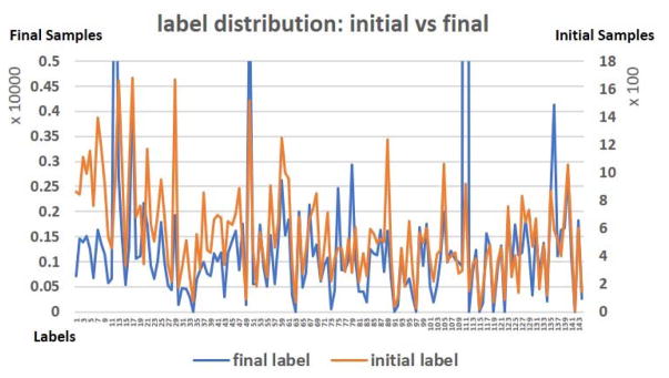
Here, in this paper, the core idea of weak initialization for the IO-CNN is to use spatial overlap rate to roughly model the training data label distribution, and then optimize the distribution through IO-CNN training. The initial and final 144 label distributions are shown in Fig. 8. The Pearson correlation between the 144 initial label distribution and the final label distribution is 0.23, which shows some level of correlation between the initial and final label distributions. Also, the p-value of the Pearson correlation is 0.0058, which is much smaller than the significance level 1%, indicating that the positive correlation between the initial and final label distributions is confident and significant. The significant correlation between the rough label distribution and the optimized label distribution cross-validated the plausibility of using overlap rate label initialization (~85% accuracy) and the optimization of IO-CNN based on that label initialization.

Fig. 8.

Initial label distribution and final label distribution after iterative IO-CNN optimization.

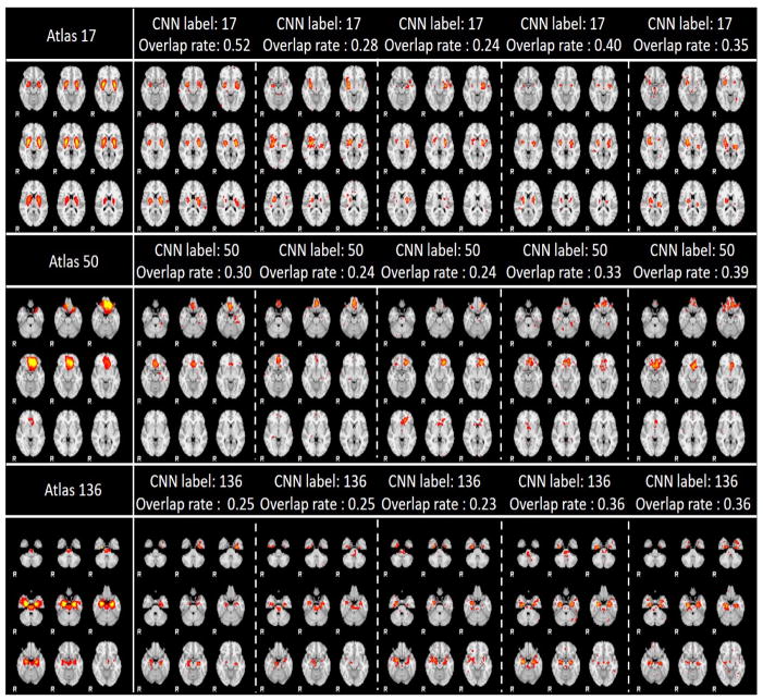
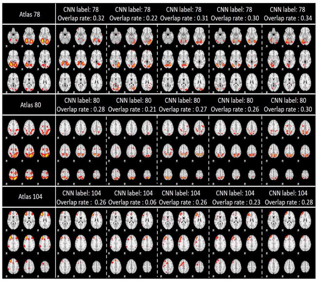
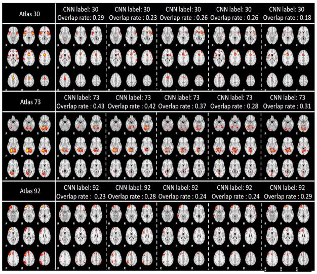
Due to the limited space, we only showcased 9 networks recognition results here using 3 labels with the most data distributions, 3 labels with medium data distributions, and 3 labels with the smallest data distributions in Fig. 9. As showcased in Fig. 9, the IO-CNN can really achieve accurate predictions for each network atlas label, which are demonstrated by both visual check and the high overlap rates of the individual networks with the corresponding atlases. The entire predictions for 219,800 networks for all of the 144 network atlas labels are visualized at our website: http://hafni.cs.uga.edu/144templates_CNN/Init-to-itr12/web/predictions. As shown in Fig. 8, the final label 111 exhibits a pulse distribution after convergence. We examined this phenomenon and found that most network belonging to this label are noisy components. Examples are shown in Supplemental Fig. 1. Furthermore, in order to test the robustness of the trained framework to avoid the overfitting on the training dataset, 200 subjects’ functional networks from ABIDE I dataset used in (Y. Zhao et al., 2016) is also tested, and the predictions are consistent with the results on the ABIDE II dataset. Comprehensive predictions are referred to http://hafni.cs.uga.edu/144templates_CNN/ABIDE-I_validation/pics/webs/. Randomly selected exemplar predictions on ABIDE I dataset are shown in Supplemental Fig. 2 (a–c) in correspondence to Fig. 9(a–c).

Fig. 9.

Fig. 9. (a). 3 label predictions with the most data distributions using 5 instances each. Each row contains the atlas picture at the first column, with the rest 5 columns as prediction instances from different individual subjects’ networks.

Fig. 9. (b). 3 label predictions with the medium data distributions using 5 instances each. Each row contains the atlas picture at the first column, with the rest 5 columns as prediction instances from different individual subjects’ networks.

Fig. 9. (c). 3 label predictions with the least data distribution using 5 instances each. Each row contains the atlas picture at the first column, with the rest 5 columns as prediction instances from different individual subjects’ networks.

3.3 Label Change Analysis and Evaluations

As mentioned in the previous section, an 87.5% consistency was achieved between the initial overlap labels and the final IO-CNN predicted labels. In general, the inconsistent predictions with the initial labels have 4 conditions: 1) Previously unlabeled data is assigned with this label; 2) New instance assigned with this label; 3) Label shifted from this label; 4) Label removed. We will use the two functional network atlases: atlas 7 (default mode network) and atlas 14 (lateral visual area network) for the 4-condition label change analysis in the following sections in details. The comprehensive 144-atlas label changes are visualized at http://hafni.cs.uga.edu/144templates_CNN/Init-to-itr12/web/, where condition 1 is linked to “new label added from no label”, condition 2 is linked to “new labels added for each template from other labels”, condition 3 is linked to “new labels removed from each template”, and condition 4 is linked to “label removed from each template”. We will explain these 4 conditions one by one in details as follows.

Condition 1)

Previously unlabeled data assigned with this label. Intuitively, most label changes come from this condition since the initial labeled size is only 80,293, compared to the final label size of 219,433. Since we set an overlap rate threshold of 0.2 empirically according to (Y. Zhao et al., 2016) to assign initial label, some functionally meaningful networks with lower spatial overlap rate than 0.2 were then discarded. Fortunately, those networks were then assigned back with a reasonable label using our trained IO-CNN model. A few randomly selected showcases using atlas 7 and 14 are illustrated in Fig. 10. The comprehensive 144-atlas label changes for this condition are visualized at http://hafni.cs.uga.edu/144templates_CNN/Init-to-itr12/web/added_from_no_label/index.html.

Fig. 10.

Previously unlabeled network assigned with label 7 and 14. The overlap rate with those networks are all below 0.2 yielding no label initially.

Condition 2)

New instance assigned with this label. This condition indicated that the current label is more suitable for the previous label assigned by using the overlap rate scheme.

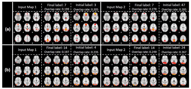
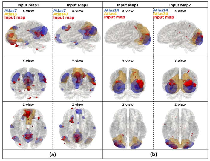
A few randomly selected showcases still using atlas 7 and 14 are illustrated in Fig. 11, and the corresponding 3D visualizations are shown in Fig. 12. From the visualization, we can confidently see the improved final label predictions, even though the spatial overlap rate is higher in initial labels than final label, which demonstrated that the spatial overlap rate is incapable of differentiating networks with high overlap rates. The 3D visualizations offer a better visualization of the spatial distribution of the input maps of activation areas, thus confirming that input maps match better with the final labels instead of initial labels. This improvement is the optimization result of our proposed IO-CNN framework and can be extensively illustrated by the comprehensive 144-atlas label change visualization for this condition at http://hafni.cs.uga.edu/144templates_CNN/Init-to-itr12/web/added_in_new/index.html.

Fig. 11.

(a). New instances with initial labels 3, 47 assigned with final label 7; (b). New instances with initial labels 4, 24 assigned with final label 14. First column of each subplot indicates input networks; second column indicates final predicted atlases; third column indicates initial overlap rate assigned labels.

Fig. 12.

(a). 3 axis 3D visualization for new instances with initial labels 3, 47 assigned with final label 7; (b). 3 axis 3D visualization for new instances with initial labels 4, 24 assigned with final label 14.

Condition 3)

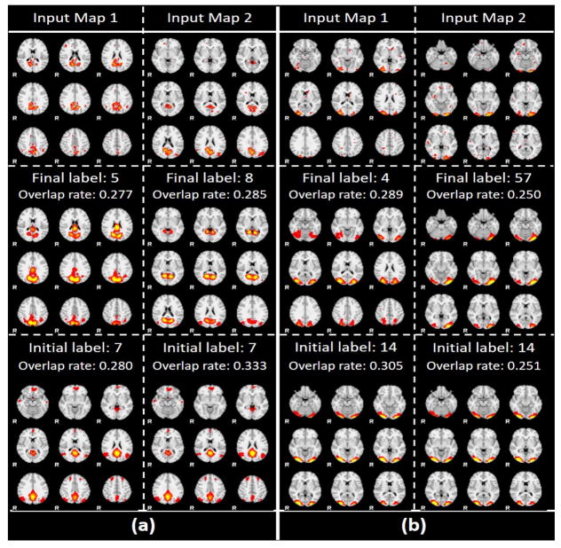
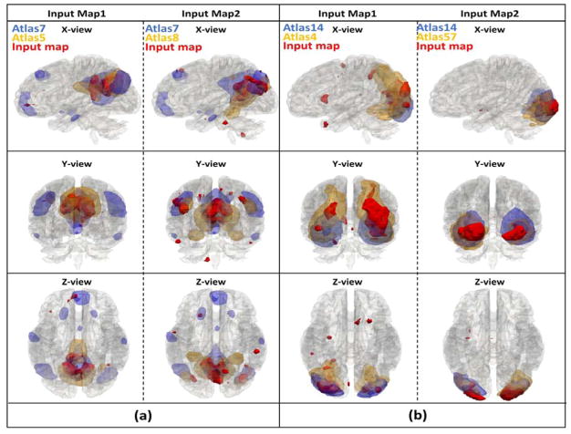
Label shifted from this label. This condition also indicated that the current label is more suitable for the previous label assigned using overlap rate scheme. Several randomly selected showcases still using atlas 7 and 14 are illustrated in Fig. 13, and the corresponding 3D visualizations are shown in Fig. 14. Similar to condition 2), we can clearly see the plausibility of the final predicted labels when the initial label atlas and final label atlas have a high overlap rate. For instance, for input map 2 in Fig. 13 and Fig. 14(b), we somehow have difficulties in telling the difference between the highly overlapped atlases 14 and 57. However, if we observe closely, we will find that the spatial distributions of the two high overlapped atlases are different: atlas 57 has a unbalanced lateral activated regions, while atlas 14 has a balanced lateral activated regions. And our final label for input map 2 is atlas 57 because the input map also has a clearly unbalanced lateral activation pattern, which should be assigned with a label 57. The extensive illustrations of comprehensive 144-atlas label changes for this condition are visualized at http://hafni.cs.uga.edu/144templates_CNN/Init-to-itr12/web/removed_from_old/index.html

Fig. 13.

(a). Label shifted from label 7 to label 5, 8; (b). Label shifted from label 14 to label 4, 57. First row of pictures indicates input networks; second row indicates final predicted atlases; third row indicates initial overlap rate assigned.

Fig. 14.

(a). 3 axis 3D visualization for instances with label shifted from label 7 to label 5, 8; (b). 3 axis 3D visualization for instances with label shifted from label 14 to label 4, 57.

Condition 4)

Label removed. This condition indicated that the label was removed (recognized as noisy network) for a network which was initially assigned with a label. Usually this condition should not happen, since if a network was assigned with an initial label, meaning the overlap rate of this network is at least 0.2 with some atlases, which indicates non-noisy network. As a result, only one initial network in atlas 7 class is removed, and there is no such condition for atlas 14. As expected, this condition does not exist in most of the atlases http://hafni.cs.uga.edu/144templates_CNN/Init-to-itr12/web/removed_in_this_label/index.html.

3.4 Revealing Fine Granularity Networks From 10 RSNs and Ambiguity Removal using HCP Dataset

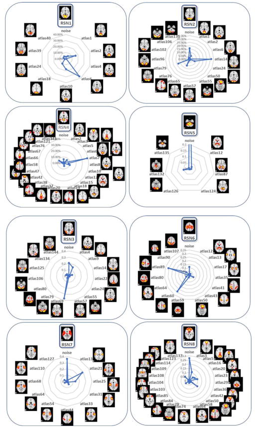
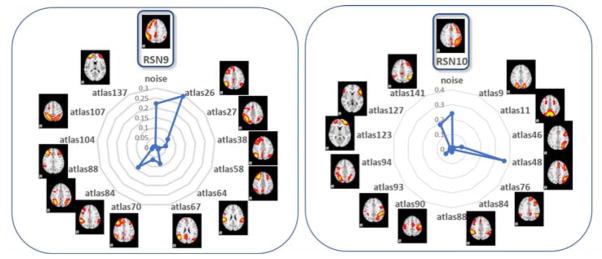
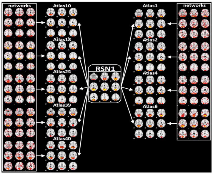
The Human Connectome Project (HCP) fMRI dataset is considered as a systematic and comprehensive mapping of connectome-scale functional networks and core nodes over a large population in the literature (Barch et al., 2013), based on which we have a classification framework for previously reported 10 resting state networks (RSN) (Smith et al., 2009) (Zhao et al., 2017b). In this section, we re-classified the 1,521 testing dataset networks from the previous HCP dataset [36]. After the predictions using the proposed 135 (from initial 144) atlas prediction framework compared with the previous 10 RSNs, we found that our 135 atlases are actually variants of the 10 RSNs with fine-granularities. Also, we further confirmed the previous framework using CNN has discovered manual labeling mistakes. As we can see from Fig. 15, the most percentage (except noises) of the atlas from 135 atlases resemble the corresponding atlases in 10 RSNs, which demonstrated the robustness of the proposed framework and its applicability on different fMRI data sets. Correspondingly, the spatial overlap rate of each RSN template with its granularities is shown in Table 1. The high overlap rate metrics demonstrated the strong spatial relationships between the granularities and the corresponding RSNs, which validated the granular characteristics.Fig. 16 shows an example of the fine granularities among 135 atlases of RSNs and the previous ambiguous labels using RSN 1 as an example. As shown in Fig. 16, atlases 4, 24 are not necessarily to be variants of fine granularities of RSN 1, but the reclassification atlases seem to be more reasonable and accurate than the previous RSN 1 using 10 RSN labels. And other atlases are variants of fine granularities of the RSN1. For a comprehensive and detailed reclassification of the HCP dataset, please refer to http://hafni.cs.uga.edu/144templates_CNN/forHCP/web/index.html.

Fig. 15.

Proposed 135-class predictions on previous 10-class labelled HCP testing set networks reveals fine-granularities of the variants of 10 RSNs. The radar charts show the 135 templates granular percentages out of the 10 RSN atlases.

Fig. 16.

Fine-granularities among 135 atlases and previous ambiguous labels using RSN 1 as an example.

This result cross-validated the effectiveness and the scalability of our IO-CNN framework to other datasets. And this finding of IO-CNN derived fine granularity of functional brain networks is also consistent with prior results in (Zhao et al., 2017a), providing neuroscientific basis for hierarchical and overlapping architecture of the human brain functions.

4. DISCUSSION AND CONCLUSIONS

Connectome-scale reconstruction of reproducible and meaningful functional brain networks on large-scale populations based on fMRI data are enabled by using functional brain network decomposition techniques, especially the HAFNI project [8]. However, an unsolved problem in the HAFNI framework is the automatic recognition of hundreds of HAFNI maps such as RSNs in each individual brain, which is challenging due to the lack of functional brain atlases, no correspondence across decomposed or reconstructed networks across different subjects, and the significant individual variabilities. To deal with the tremendous variability of various types of functional brain networks and the presence of various sources of noises, we have proposed a 3D CNN deep learning framework to solve those problems [35]. However, major challenges like labelling large scale networks and recognition of them with larger scale labels still remain prominent. The previous 3D CNN framework is extended in this work for much larger networks recognitions (from ~5,000 to ~220,000) with much larger numbers of network atlases (from 10 to 135) with a weak but automatic labeling. The recognition results and the label changes from initial labels by our IO-CNN framework demonstrated the optimization during iterative training. The application of IO-CNN on the separate HCP dataset with previous 10 RSN labels obtained promising results, in which functional network fine-granularities and label ambiguity removal have been achieved, further demonstrating the robustness and efficiency of our proposed IO-CNN framework. In the future, we will further refine the collection of comprehensive and holistic functional brain network atlases together with an effective recognition system, and then apply them on clinical fMRI datasets for brain disease modelling, such as for Alzheimer’s disease and Autism Spectrum Disorder.

Fig. 3.

IO-CNN framework. (a). weak label initialization process based on spatial overlap rate; (b). iteratively optimized CNN (IO-CNN) training process. The training process will iterate over the 219,800 input 3D maps starting with the initial weak labels. Only the 3D maps with nonzero labels will be taken as input for the current training iteration. After each training iteration, the trained model will predict on all the 219,800 training samples for new labels, which will be used to replace and update the previous training labels for the next training iteration. Meanwhile, the label differences between the previous training labels and the new predicted labels will be recorded for iteration termination condition check.

References

- Barch DM, Burgess GC, Harms MP, Petersen SE, Schlaggar BL, Corbetta M, Glasser MF, Curtiss S, Dixit S, Feldt C, Nolan D, Bryant E, Hartley T, Footer O, Bjork JM, Poldrack R, Smith S, Johansen-Berg H, Snyder AZ, Van Essen DC WU-Minn HCP Consortium. Function in the human connectome: task-fMRI and individual differences in behavior. Neuroimage. 2013;80:169–89. doi: 10.1016/j.neuroimage.2013.05.033. [DOI] [PMC free article] [PubMed] [Google Scholar]
- Bengio Y, Courville A, Vincent P. Representation Learning: A Review and New Perspectives. IEEE Trans Pattern Anal Mach Intell. 2013;35:1798–1828. doi: 10.1109/TPAMI.2013.50. [DOI] [PubMed] [Google Scholar]
- Cole DM, Smith SM, Beckmann CF. Advances and pitfalls in the analysis and interpretation of resting-state FMRI data. Front Syst Neurosci. 2010;4:8. doi: 10.3389/fnsys.2010.00008. [DOI] [PMC free article] [PubMed] [Google Scholar]
- Fox MD, Snyder AZ, Vincent JL, Corbetta M, Van Essen DC, Raichle ME. The human brain is intrinsically organized into dynamic, anticorrelated functional networks. Proc Natl Acad Sci U S A. 2005;102:9673–8. doi: 10.1073/pnas.0504136102. [DOI] [PMC free article] [PubMed] [Google Scholar]
- Friston KJ, Holmes AP, Worsley KJ, Poline JP, Frith CD, Frackowiak RSJ. Statistical parametric maps in functional imaging: A general linear approach. Hum Brain Mapp. 1994;2:189–210. doi: 10.1002/hbm.460020402. [DOI] [Google Scholar]
- Han J, Ji X, Hu X, Guo L, Liu T. Arousal Recognition Using Audio-Visual Features and FMRI-Based Brain Response. IEEE Trans Affect Comput. 2015;6:337–347. doi: 10.1109/TAFFC.2015.2411280. [DOI] [Google Scholar]
- Harris KD, Mrsic-Flogel TD. Cortical connectivity and sensory coding. Nature. 2013;503:51–58. doi: 10.1038/nature12654. [DOI] [PubMed] [Google Scholar]
- He K, Zhang X, Ren S, Sun J. Delving Deep into Rectifiers: Surpassing Human-Level Performance on ImageNet Classification 2015 [Google Scholar]
- Huang H, Hu X, Zhao Y, Makkie M, Dong Q, Zhao S, Guo L, Liu T. Modeling Task fMRI Data via Deep Convolutional Autoencoder. IEEE Trans Med Imaging. 2017:1–1. doi: 10.1109/TMI.2017.2715285. [DOI] [PubMed] [Google Scholar]
- Ioffe S, Szegedy C. Batch Normalization: Accelerating Deep Network Training by Reducing Internal Covariate Shift 2015 [Google Scholar]
- Jenkinson M, Beckmann CF, Behrens TE, Woolrich MW, Smith SM. FSL. Neuroimage. 2012;62:782–90. doi: 10.1016/j.neuroimage.2011.09.015. [DOI] [PubMed] [Google Scholar]
- Deng Jia, Dong Wei, Socher R, Li Li-Jia, Li Kai, Fei-Fei Li. ImageNet: A large-scale hierarchical image database. 2009 IEEE Conference on Computer Vision and Pattern Recognition; IEEE; 2009. pp. 248–255. [DOI] [Google Scholar]
- Karpathy A, Toderici G, Shetty S, Leung T, Sukthankar R, Fei-Fei L. Large-scale Video Classification with Convolutional Neural Networks. The IEEE Conference on Computer Vision and Pattern Recognition (CVPR); 2014. pp. 1725–1732. [Google Scholar]
- Krizhevsky A, Sutskever I, Hinton GE. ImageNet Classification with Deep Convolutional Neural Networks, NIPS. 2012. [Google Scholar]
- Lawrence S, Giles CL, Tsoi Ah Chung, Back AD. Face recognition: a convolutional neural-network approach. IEEE Trans Neural Networks. 1997;8:98–113. doi: 10.1109/72.554195. [DOI] [PubMed] [Google Scholar]
- LeCun Y, Bengio Y, Hinton G. Deep learning. Nature. 2015;521:436–444. doi: 10.1038/nature14539. [DOI] [PubMed] [Google Scholar]
- Lecun Y, Eon Bottou L, Bengio Y, Haaner P. Gradient-Based Learning Applied to Document Recognition RS-SVM Reduced-set support vector method. SDNN Space displacement neural network. SVM Support vector method. TDNN Time delay neural network. V-SVM Virtual support vector method. PROC IEEE 1998 [Google Scholar]
- Logothetis NK. What we can do and what we cannot do with fMRI. Nature. 2008;453:869–78. doi: 10.1038/nature06976. [DOI] [PubMed] [Google Scholar]
- Lv J, Jiang X, Li X, Zhu D, Chen H, Zhang T, Zhang S, Hu X, Han J, Huang H, Zhang J, Guo L, Liu T. Sparse representation of whole-brain fMRI signals for identification of functional networks. Med Image Anal. 2015a;20:112–34. doi: 10.1016/j.media.2014.10.011. [DOI] [PubMed] [Google Scholar]
- Lv J, Jiang X, Li X, Zhu D, Zhang S, Zhao S, Chen H, Zhang T, Hu X, Han J, Ye J, Guo L, Liu T. Holistic atlases of functional networks and interactions reveal reciprocal organizational architecture of cortical function. IEEE Trans Biomed Eng. 2015b;62:1120–31. doi: 10.1109/TBME.2014.2369495. [DOI] [PubMed] [Google Scholar]
- Lv J, Jiang X, Li X, Zhu D, Zhao S, Zhang T, Hu X, Han J, Guo L, Li Z, Coles C, Hu X, Liu T. Assessing effects of prenatal alcohol exposure using group-wise sparse representation of fMRI data. Psychiatry Res. 2015c;233:254–68. doi: 10.1016/j.pscychresns.2015.07.012. [DOI] [PMC free article] [PubMed] [Google Scholar]
- Lv J, Li X, Zhu D, Jiang X, Zhang X, Hu X, Zhang T, Guo L, Liu T. Sparse representation of group-wise FMRI signals. Med Image Comput Comput Assist Interv. 2013;16:608–16. doi: 10.1007/978-3-642-40760-4_76. [DOI] [PubMed] [Google Scholar]
- Maas AL, Hannun AY, Ng AY. ICML. 2013. Rectifier Nonlinearities Improve Neural Network Acoustic Models. [Google Scholar]
- Mairal J, Bach F, Ponce J, Sapiro G. Online Learning for Matrix Factorization and Sparse Coding. J Mach Learn Res. 2010;11:19–60. [Google Scholar]
- McKeown MJ, Hansen LK, Sejnowsk TJ. Independent component analysis of functional MRI: what is signal and what is noise? Curr Opin Neurobiol. 2003;13:620–629. doi: 10.1016/j.conb.2003.09.012. [DOI] [PMC free article] [PubMed] [Google Scholar]
- Liu Nian, Han J, Zhang D, Wen Shifeng, Liu T. Predicting eye fixations using convolutional neural networks. 2015 IEEE Conference on Computer Vision and Pattern Recognition (CVPR); IEEE; 2015. pp. 362–370. [DOI] [Google Scholar]
- Scherer D, Müller A, Behnke S. ICANN. Springer; Berlin, Heidelberg: 2010. Evaluation of Pooling Operations in Convolutional Architectures for Object Recognition; pp. 92–101. [DOI] [Google Scholar]
- Schmidhuber JJ. Deep learning in neural networks: An overview. Neural Networks. 2014;61:85–117. doi: 10.1016/j.neunet.2014.09.003. [DOI] [PubMed] [Google Scholar]
- Simonyan K, Zisserman A. Very Deep Convolutional Networks for Large-Scale Image Recognition. 2014. [Google Scholar]
- Smith SM, Fox PT, Miller KL, Glahn DC, Fox PM, Mackay CE, Filippini N, Watkins KE, Toro R, Laird AR, Beckmann CF. Correspondence of the brain’s functional architecture during activation and rest. Proc Natl Acad Sci U S A. 2009;106:13040–5. doi: 10.1073/pnas.0905267106. [DOI] [PMC free article] [PubMed] [Google Scholar]
- Xu J, Potenza MN, Calhoun VD, Zhang R, Yip SW, Wall JT, Pearlson GD, Worhunsky PD, Garrison KA, Moran JM. Large-scale functional network overlap is a general property of brain functional organization: Reconciling inconsistent fMRI findings from general-linear-model-based analyses. Neurosci Biobehav Rev. 2016;71:83–100. doi: 10.1016/j.neubiorev.2016.08.035. [DOI] [PMC free article] [PubMed] [Google Scholar]
- Zeiler MD. ADADELTA: An Adaptive Learning Rate Method. 2012. [Google Scholar]
- Zhao S, Han J, Jiang X, Hu X, Lv J, Zhang S, Ge B, Guo L, Liu T. Exploring auditory network composition during free listening to audio excerpts via group-wise sparse representation. 2016 IEEE International Conference on Multimedia and Expo (ICME); IEEE; 2016. pp. 1–6. [DOI] [Google Scholar]
- Zhao Y, Chen H, Li Y, Lv J, Jiang X, Ge F, Zhang T, Zhang S, Ge B, Lyu C, Zhao S, Han J, Guo L, Liu T. Connectome-scale group-wise consistent resting-state network analysis in autism spectrum disorder. NeuroImage Clin. 2016;12:23–33. doi: 10.1016/j.nicl.2016.06.004. [DOI] [PMC free article] [PubMed] [Google Scholar]
- Zhao Y, Dong Q, Chen H, Iraji A, Li Y, Makkie M, Kou Z, Liu T. Constructing fine-granularity functional brain network atlases via deep convolutional autoencoder. Med Image Anal. 2017a;42:200–211. doi: 10.1016/j.media.2017.08.005. [DOI] [PMC free article] [PubMed] [Google Scholar]
- Zhao Y, Dong Q, Zhang S, Zhang W, Chen H, Jiang X, Guo L, Hu X, Han J, Liu T. Automatic Recognition of fMRI-derived Functional Networks using 3D Convolutional Neural Networks. IEEE Trans Biomed Eng. 2017b:1–1. doi: 10.1109/TBME.2017.2715281. [DOI] [PMC free article] [PubMed] [Google Scholar]
Associated Data
This section collects any data citations, data availability statements, or supplementary materials included in this article.