SHARD: Spherical Harmonic-based Robust Outlier Detection for HARDI Methods

Abstract

High Angular Resolution Diffusion Imaging (HARDI) models are used to capture complex intra-voxel microarchitectures. The magnetic resonance imaging sequences that are sensitized to diffusion are often highly accelerated and prone to motion, physiologic, and imaging artifacts. In diffusion tensor imaging, robust statistical approaches have been shown to greatly reduce these adverse factors without human intervention. Similar approaches would be possible with HARDI methods, but robust versions of each distinct HARDI approach would be necessary. To avoid the computational and pragmatic burdens of creating individual robust HARDI analysis variants, we propose a robust outlier imputation model to mitigate outliers prior to traditional HARDI analysis. This model uses a weighted spherical harmonic fit of diffusion weighted magnetic resonance imaging scans to estimate the values which had been corrupted during acquisition to restore them. Briefly, spherical harmonics of 6^th order were used to generate basis function which were weighted by diffusion signal for detection of outliers. For validation, a single healthy volunteer was scanned for a single session comprising of two scans one without head movement and the other with deliberate head movement at a b-value of 3000 s/mm² with 64 diffusion weighted directions with a single b0 (5 averages) per scan. The deliberate motion from the volunteer created natural artifacts in the acquisition of one of the scans. The imputation model shows reduction in root mean squared error of the raw signal intensities and improvement for the HARDI method Q-ball in terms of the Angular Correlation Coefficient. The results reveal that there is quantitative and qualitative improvement. The proposed model can be used as general pre-processing model before implementing any HARDI model in general to restore the artifacts which are created because of the outlier diffusion signal in certain gradient volumes.

1. INTRODUCTION

Diffusion weighted magnetic resonance imaging (DW-MRI) measurements provide contrasts sensitive to the microarchitectural environment at a millimeter scale. The data have been widely used to model brain structural connectivity using diffusion tensor imaging (DTI) [1]. However, DTI is limited in that it only provides a single fiber/peak orientation per voxel. More recent methods which can be labelled collectively as high angular resolution diffusion imaging (HARDI) provide models capturing information on the existence of multiple fiber orientations per voxel. Yet, HARDI is not a singular technique; rather, numerous methods exist to model DW-MRI data with more complex intra-voxel models such as Q-ball, spherical deconvolution, PAS-MRI, diffusion orientation transform [2–6].

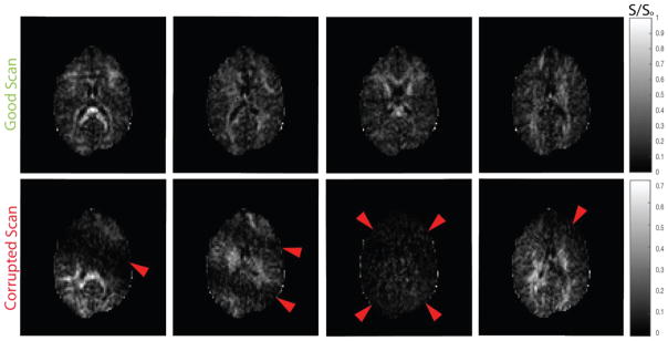
Generally, acquisitions consisting of 45 or more diffusion weighted volumes can be termed as HARDI acquisitions [7]. With increased number of gradient volumes per acquisition the probability of artifacts that might invade the acquisition also increases. Artifacts occur not only due to noise or system instabilities of a scanner but also from physiological motion of the subject [8], e.g., signal dropout, signal intensity spike, ghosting and striping (see Fig 1). A single artifact in a gradient volume can be detrimental for voxel-wise fitting methods and can lead to increased bias and variance for the methods. It has been shown that a single corrupted gradient volume for a HARDI acquisition can introduce an error of approximately 10% in Fractional Anisotropy (FA) and General Fractional Anisotropy (GFA) [9] using robust spherical harmonics Q-ball imaging [5]. Generally, the practical quality control advice for DW-MRI is to either remove gradient volumes or perform correction using interpolation techniques [9]. Hence, it is critically important for the artifacts to be detected and either removed or imputed for reduction of bias in HARDI methods.

Figure 1.

Comparison of good and corrupted scan data from an empirical in vivo acquisition. The red arrows in the second row highlight areas of artifact.

Previous work on robust estimation of DTI has been characterized with weighted least squares fit and robust M-estimators [10, 11]. Briefly, outlier detection models have been designed to exclude and then compute DTI with the remaining measurements. Subsequently, iteratively reweighted linear least squares (IRLLS) were developed to increase the speed with DTI [12]. To date, a consensus has not been reached for HARDI outlier detection. One approach uses compressed sensing on q-space resampling as an alternative to excluding gradient volumes [13], which is effective when there is signal dropout because of bulk motion. An adaption of the robust estimation of tensors by outlier rejection (RESTORE) [10] uses spherical harmonics for outlier detection and exclusion, higher order model outlier rejection (HOMOR) [14]. HOMOR is effective at removing outliers at higher b-values (up to 3000 s/mm² where RESTORE suggests invalid outliers), while HOMOR maintains similar performance to RESTORE at lower/clinical b-values. Outlier detection and replacement has also been incorporated in the non-parametric framework of eddy [15]. Eddy’s non-parametric model achieves superior performance over RESTORE [16]. Here we focus on outlier detection independent of registration and distortion correction. In light of the advanced work with tensors, one could construct statistically robust variants of each traditional HARDI model. However, such efforts would require specific coding for each HARDI variant and potentially dramatically increased computational times given the need for re-computation of fitting procedures on a voxel-wise basis. Here, we follow in HOMOR’s approach for outlier detection using an iterative linear least squares model, but our approach uses residual based re-weighting with a ridge regression with L2 penalty. HOMOR does not impute the data and is a detection technique while our approach is both a detection and replacement model on a voxel by voxel basis.

Here, we propose a robust outlier imputation model that uses an iterative regularized weighted linear least squares (IRWLLS) fit which functions per voxel. The IRWLLS model uses even order weighted spherical harmonics which can be used to calculate residuals with the original signal intensities. The weights are based on squared residuals and squared standard deviation (SD) of residual between signal intensities and regular spherical harmonics across the entire acquired volume of the brain. Based on a certain threshold multiplied with the SD of the entire brain residuals, the outliers can be detected and imputed with weighted spherical harmonic intensities. This work reveals that an imputation model can be useful for detecting artifacts and it minimizes error when compared with an in vivo acquired ground truth (good scan). In an empirical demonstration, the improvement is noticeable for Q-ball in terms of angular correlation coefficients.

2. METHODS

2.1 DW-MRI Data Measurements and Pre-Processing

A single healthy volunteer was scanned for a single session at 3T (Achieva, Philips Medical System Systems, Best, The Netherlands) with a 32-channel head coil. Two scans were acquired each with 64 gradient direction for a b-value of 3000 s/mm² each with a minimally weighted reference (b0). Acquisition parameters voxel resolution=2.5×2.5×2.5 mm³ Multi-Band=2; SENSE=2.2; TR= 2650 ms; TE=94 ms; partial Fourier=0.7. In one of the two scans, the volunteer was specifically asked to move their head at random intervals. This was done to introduce artifacts in the acquired scan. One third of the gradient volumes show major artifacts in the middle axial slice and can be noticed easily visually (refer Fig 1).

The acquired data were preprocessed for patient movement, eddy current distortions and susceptibility distortion using eddy and topup [15, 17]. The b0’s were concatenated together and fed as input to topup. Both the scans were concatenated together and then used as input to topup which was pipelined to eddy. The corrected data from eddy were successively registered to the b0’s using flirt [18, 19]. The two scans were normalized by the corresponding b0 to account for the amplitude drift.

2.2 SHARD Algorithm

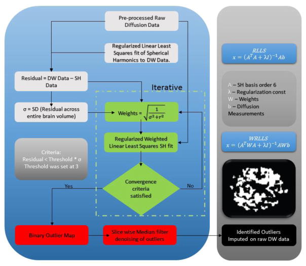
The pre-processed data was fitted to spherical harmonics of order 6 to generate 28 basis functions. The SD was calculated of the residuals between the DW-MRI data signal intensities (S/S_o) and the spherical harmonic fitted signal intensities for both the scans (σ) (Figure 2). The spherical harmonic basis functions were fitted to DW-MRI using a regularized linear least squared fit (RLLS) and is also known as a ridge regression with L2 penalty. Regularization constant was fixed at 0.005 as the known used value from Q-ball. This algorithm functions on a voxel by voxel basis iteratively. Weights have been calculated as square root of inverse of sum of squares of σ and residual per voxel leading to an equivalent number of weights as the gradient directions. The original DW-MRI data are fitted using weighted spherical harmonics basis functions of order 6. A weighted regularized linear least squared fit (WRLLS) has been used iteratively till the convergence criteria are satisfied. The criteria were set to three deviations of σ for the residual. Failure of satisfaction of the criteria leads to recalculation of weights using any signals that were imputed. At every iteration, the outlier binary map is updated. Once the procedure has been completed for the entire brain volume a final outlier map is generated. This outlier map is denoised/interpolated using a two-dimensional median filter to get rid of spurious outliers that were detected during the iterations of the SHARD algorithm. Denoised outlier map is used for imputation of the original DW-MRI measurements which are replaced by the sampled weighted spherical harmonic signals for the true outliers that were detected. This algorithm can be used for either exclusion or imputation functionality or for both. However, in regards to this work it has been used an exclusion and imputation model.

Figure 2.

SHARD Algorithm’s iterative pipeline. The first phase of SHARD (white boxes), involves a regularized spherical harmonic fit to the preprocessed diffusion data, which enables estimation of the standard deviation of the model fit across the brain (σ). The second phase (green boxes) uses iterative reweighted spherical harmonic fitting to identify and de-weight outliers on a voxelwise basis. Finally (red boxes), outliers are identified from the reweighted spherical harmonic fit, median filtered, and imputed with their model fit values. The resulting data can be used in subsequent HARDI model processing (black box).

2.3 Validation of SHARD in Simulation

The ground truth (good scan) was taken and artificial noise was added per voxel at gradient directions that were chosen randomly. ‘S’ defines the signal intensity for a diffusion weighted volume while ‘S_o’ defines a non-weighted diffusion volume. For a randomly chosen gradient direction a probability (p) was randomly generated. If p >= 0.5 then the corruption factor was used to divide S/S_o and if it was p < 0.5 then corruption factor was used to multiply S/S_o. This experiment was repeated 64 times per corrupted direction while increasing number of corrupted directions up to the maximum number of gradient directions that were acquired with this data set. This synthetic corruption model has been labelled as ‘Slash Model’ for future reference and in the figures as well. We used a two-step validation process the first one being the root mean squared error measured against the ground truth across all the signal intensities (S/S_o) over the entire brain volume comprising of all gradient directions (1). ‘G’ is the total number of gradient directions and ‘N’ is the total number of slices that were acquired.

$$\mathit{RMSE}\left(\frac{S}{S_o}\right)=\sqrt{\frac{{\mathrm{\sum }}_1^G{\mathrm{\sum }}_1^N{(\frac{S}{S_o}(\mathit{truth})-\frac{S}{S_o}(\mathit{imputed}))}^2}{G·N}}$$ (1)

The second step validation is using angular correlation coefficient (ACC) which is based on the coefficients of the HARDI method Q-ball (2). ACC is a convenient way for calculating correlations of functions of all directions over a spherical harmonic expansion. It provides an estimate of how closely two orientation distribution functions (ODF) relate to each other. It was first estimated on a voxel by voxel basis. ‘u’ is the test function of Q-ball coefficients while ‘v’ is the true set of Q-ball coefficients from the ground truth (good scan) data. It can be inferred that the ACC if taken between two separately calculated Q-ball coefficients from ground truth data its value will be equivalent to 1. This was empirically determined as well. This metric has been represented across the entire brain volume using RMSE and the mean.

$$\mathit{ACC}=\frac{{\mathrm{\sum }}_{j=1}^{\propto }{\mathrm{\sum }}_{m=-j}^j{u}_{jm}{v}_{jm}^{\ast }}{{\left[{\mathrm{\sum }}_{j=1}^{\propto }{\mathrm{\sum }}_{m=-j}^j{\left|u_{jm}\right|}^2\right]}^{0.5}·{\left[{\mathrm{\sum }}_{j=1}^{\propto }{\mathrm{\sum }}_{m=-j}^j{\left|v_{jm}\right|}^2\right]}^{0.5}}$$ (2)

When performing this robust experiment on the ground truth (good scan) and the motion scan data the same methodology as above has been used. However instead of multiplying or dividing signal intensities by a corruption factor, random permutations of the gradient volumes were chosen from the motion scan data. The permutations ranging from 1 to 64. At each level of corrupted directions, the experiment was repeated 64 times for robustness.

3. RESULTS

3.1 True and False Positive

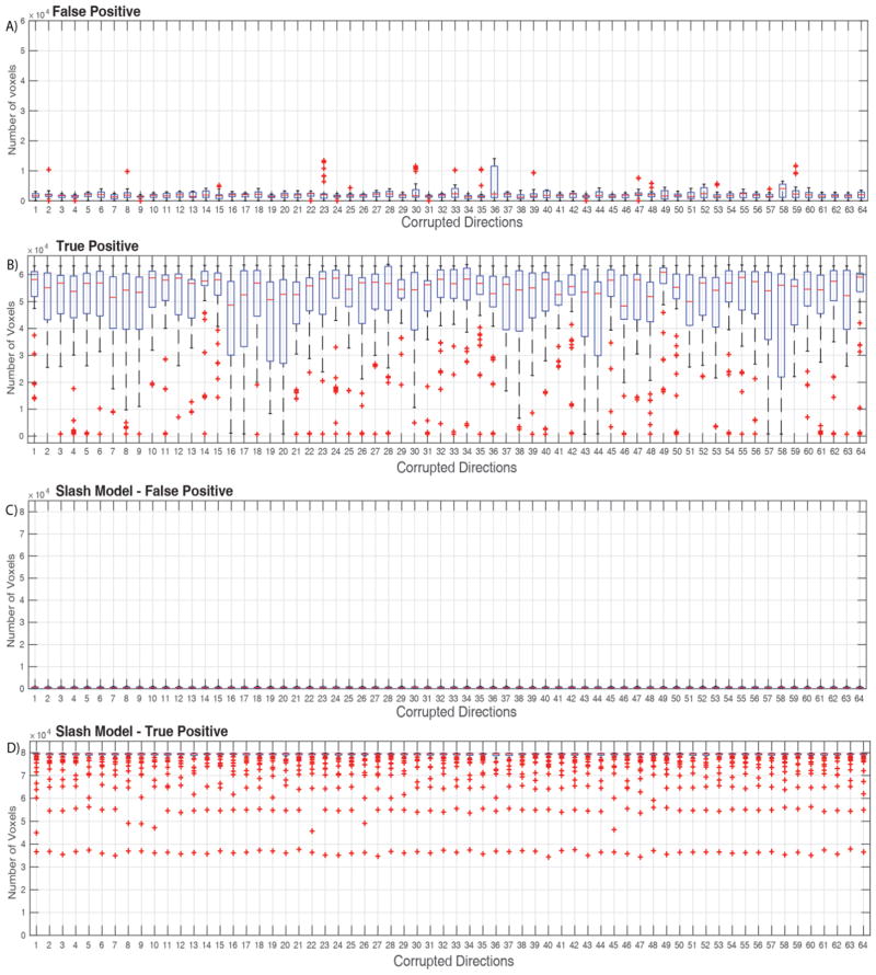
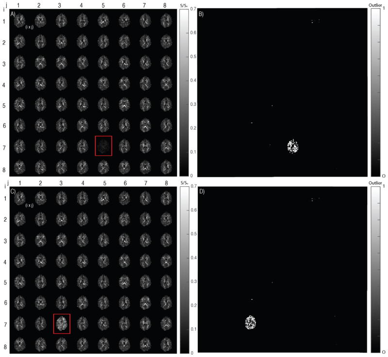
True positives have been defined as outliers that are correctly identified by the model (true outliers are known because they are simulated) while false are the ones that are detected but they are not in actual. The number of false positives being detected for both the slash model and when tested with motion scan data are close to a 1000 voxels combined across all the uncorrupted gradient volumes (Figure 4A and 4C). Specifically, when motion corrupted scan volumes are swapped, it is noticeable that there are visual inconsistencies. The true positives in the corrupted gradient volumes are consistently greater and at a much higher ratio than the number of false positives being detected (Figure 4B and 4D). The number of true positives drop in cases of certain corrupted volumes and are accounted to gradient volumes that are not corrupt in the motion scan data. The ratio is ~1:60 when using motion data scan to introduce corruption. The ratio is even higher in the scenario of slash model true positives and false positives. Qualitatively, the above-mentioned result is re-enforced as it is apparent to notice that there are fewer outliers being detected in the uncorrupted gradient volumes (Figure 3B and 3D). This result is regardless of slash model corruption of volumes or swapping corrupted volumes from motion scan data.

Figure 4.

Count of outliers detected in corrupted gradient volumes (True Positive) and uncorrupted gradient volumes (False Positive). Each bin consists of 64 repeated measurements. Total number of voxels per volume are 92,248. A) False positive, outliers detected in the uncorrupted gradient volume when using corrupted gradient volumes from motion scan. B) True Positive, outliers detected in the uncorrupted gradient volumes which has random volumes swapped in from the motion scan. C) False positive, outliers detected in the uncorrupted gradient volume when using Slash model corruption factor for random gradient volumes. D) True Positive, outliers detected in gradient volumes when using Slash model corruption factor for random gradient volumes.

Figure 3.

Middle axial slice shown for the diffusion data and the binary outlier map. i*j denotes the weighted gradient volume corresponding to gradient directions. A) Ground truth data when corrupted with an artifact containing gradient volume from the motion scan. B) Outlier detected on the corrupted gradient volume in (A). C) Simulated good scan data when corrupted artificially by random multiplication and division of signal intensity using a corruption factor (Slash Model). D) Outliers detected with the artificial corrupted gradient volume in (C).

3.2 RMSE of Signal Intensity

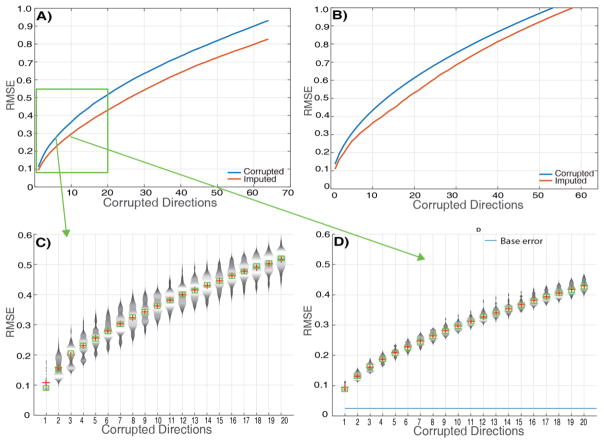
The RMSE of 64 repeated measurements with random permutations that the overall error after using this algorithm for pre-processing is always less than the original error (Figure 5A and 5B). This can be observed for both slash model corruption and motion scan corruption. A distribution plot of the 64 repeated measurements for the first 20 corrupted directions shows that either the RMSE is reduced or it is the same when compared with the original error (Figure 5C and 5D). The RMSE increases for the original corruption and after imputation with the increase of corrupted gradient directions. However, the RMSE after imputation is generally less by approximately 0.06 for the S/S_o. The base error that is introduced by SHARD in the ground truth with no corrupted volumes is approximately 0.015 for S/S_o (Figure 5D). The distribution plots show that there is a higher likelihood of having a lower RMSE as compared to original RMSE after imputation.

Figure 5.

A) RMSE of corrupted and imputed signal intensities across the brain when compared with the ground truth. Corrupted gradient volumes were swapped from the motion scan. Each point represents RMSE across 64 measurements. B) RMSE of corrupted and imputed signal intensities when compared with ground truth. Gradient volumes were corrupted with a corruption factor artificially (slash model). Each point represents RMSE across 64 measurements. C) Violin plot of 64 repeated measures of RMSE per bin with random permutations before imputation for the first 20 corrupted gradient volumes. The corrupted volumes were swapped in from motion scan data. D) Violin plot of 64 repeated measures of RMSE per bin with random permutations after imputation for the first 20 corrupted gradient volumes. The corrupted volumes were swapped in from motion scan data.

3.3 RMSE of ACC

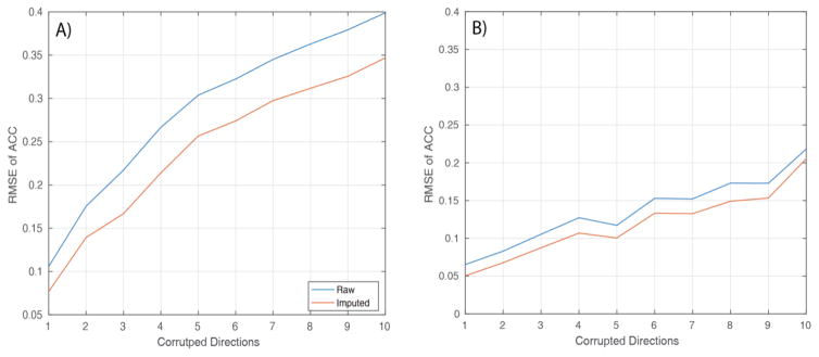
RMSE of ACC across the entire brain shows us that the error is consistently reduced when compared to the ground truth ACC (Figure 6A and 6B). This result holds true for both slash model and corruption using motion scan data. It is noticeable, however, that the error reduction in the scenario of motion scan data is comparatively lesser as compared to error reduction in slash model. The RMSE of ACC increases with increasing number of corrupted gradient directions and so does the RMSE of ACC after imputation. However, the constant error reduction can be noticed at about 0.03 for the slash model and 0.02 for the motion scan data.

Figure 6.

RMSE of ACC between spherical harmonics coefficients of Q-ball: A) between corrupted data (Slash model) and ground truth data. B) between corrupted data (motion scan data) and ground truth data.

4. DISCUSSION

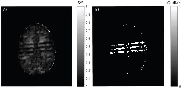
The SHARD algorithm is a promising pre-processing technique for mitigating outliers in HARDI data. The base error that has been observed in the ground truth (Figure 5D) with no corrupted volumes can be visually attributed to artifacts that are present in the ground truth “good” data (Figure 7). These artifacts can sometimes be difficult to capture with visual observation (given 44 total slices per dataset), but were detected by SHARD. SHARD’s utility appears to degrade once approximately 10 corrupted gradient volumes are introduction.

Figure 7.

A) Middle axial slice containing a striping artifact in the ground truth. B) Outlier mask detected by the SHARD model.

The usage of spherical interpolation of data has been quite popular in the recent times for [9, 14]. In this scenario while using a weighted version of spherical harmonics only a reduction 0.06 in terms of RMSE could achieved when imputing original signal intensities. There is potential room for improvement with usage of different interpolation techniques. Though there have been outlier detection models which have used spherical harmonics of order 4 [14]. A parameter optimization analysis could prove to be beneficial purely focused towards spherical harmonic orders. Another possible room for improvement is whether to introduce a weighted mean of the signal intensity along with the spherical harmonic fitted signal intensity which could further reduce the error between the original and the imputed signal.

A median filter approach slice wise has been effective but it is a two-dimensional solution. A positive improvement could be made using a three-dimensional spatial regularization which could tighten the exact outliers being detected to the specific artifact. This could lead to a crucial increment in accuracy of temporal artifacts that could possibly invade the data. At the same time doing so should also remove single spurious outliers that are detected. Labelling a single voxel as an outlier is a difficult question to answer and simply labelling them as an outlier might only lead to increment in errors between original and imputed signal. Clustering of outliers holds potential in increasing this algorithm’s efficiency.

5. CONCLUSION

The SHARD algorithm can detect sufficient outliers in corrupted gradient volumes which contain artifacts or contain signal dropout regions while not impacting the uncorrupted gradient volumes. Instead of exclusion of the detected outliers they can be safely imputed with the weighted spherical harmonic modelled signal intensities without introducing additional errors. Further validation and testing of this algorithm is necessary on a larger data set and using multiple HARDI models that are present. A comparison with the present outlier imputation techniques is clearly warranted. It would be interesting to estimate which techniques can detect and impute outliers without introducing additional errors.

References

- 1.Basser PJ, Mattiello J, LeBihan D. MR diffusion tensor spectroscopy and imaging. Biophysical journal. 1994;66(1):259–267. doi: 10.1016/S0006-3495(94)80775-1. [DOI] [PMC free article] [PubMed] [Google Scholar]
- 2.Tournier JD, et al. Direct estimation of the fiber orientation density function from diffusion-weighted MRI data using spherical deconvolution. NeuroImage. 2004;23(3):1176–1185. doi: 10.1016/j.neuroimage.2004.07.037. [DOI] [PubMed] [Google Scholar]
- 3.Jansons KM, Alexander DC. Persistent angular structure: new insights from diffusion magnetic resonance imaging data. Inverse problems. 2003;19(5):1031. doi: 10.1007/978-3-540-45087-0_56. [DOI] [PubMed] [Google Scholar]
- 4.Tuch DS. Q-ball imaging. Magnetic resonance in medicine. 2004;52(6):1358–1372. doi: 10.1002/mrm.20279. [DOI] [PubMed] [Google Scholar]
- 5.Descoteaux M, et al. Regularized, fast, and robust analytical Q-ball imaging. Magnetic resonance in medicine. 2007;58(3):497–510. doi: 10.1002/mrm.21277. [DOI] [PubMed] [Google Scholar]
- 6.Özarslan E, et al. Resolution of complex tissue microarchitecture using the diffusion orientation transform (DOT) NeuroImage. 2006;31(3):1086–1103. doi: 10.1016/j.neuroimage.2006.01.024. [DOI] [PubMed] [Google Scholar]
- 7.Tournier J, Calamante F, Connelly A. Determination of the appropriate b value and number of gradient directions for high-angular-resolution diffusion-weighted imaging. NMR in Biomedicine. 2013;26(12):1775–1786. doi: 10.1002/nbm.3017. [DOI] [PubMed] [Google Scholar]
- 8.Henkelman RM. Erratum: Measurement of signal intensities in the presence of noise in MR images [Med. Phys. 12, 232 (1985)] Medical physics. 1986;13(4):544–544. doi: 10.1118/1.595711. [DOI] [PubMed] [Google Scholar]
- 9.Sharman MA, et al. Impact of outliers on diffusion tensor and Q ball imaging: Clinical implications and correction strategies. Journal of Magnetic Resonance Imaging. 2011;33(6):1491–1502. doi: 10.1002/jmri.22577. [DOI] [PubMed] [Google Scholar]
- 10.Chang LC, Jones DK, Pierpaoli C. RESTORE: robust estimation of tensors by outlier rejection. Magnetic resonance in medicine. 2005;53(5):1088–1095. doi: 10.1002/mrm.20426. [DOI] [PubMed] [Google Scholar]
- 11.Chang LC, Walker L, Pierpaoli C. Informed RESTORE: a method for robust estimation of diffusion tensor from low redundancy datasets in the presence of physiological noise artifacts. Magnetic resonance in medicine. 2012;68(5):1654–1663. doi: 10.1002/mrm.24173. [DOI] [PMC free article] [PubMed] [Google Scholar]
- 12.Collier Q, et al. Iterative reweighted linear least squares for accurate, fast, and robust estimation of diffusion magnetic resonance parameters. Magnetic resonance in medicine. 2015;73(6):2174–2184. doi: 10.1002/mrm.25351. [DOI] [PubMed] [Google Scholar]
- 13.Elhabian S, et al. Compressive sensing based Q-space resampling for handling fast bulk motion in hardi acquisitions. Biomedical Imaging (ISBI), 2016 IEEE 13th International Symposium on; IEEE; 2016. [DOI] [PMC free article] [PubMed] [Google Scholar]
- 14.Pannek K, et al. HOMOR: higher order model outlier rejection for high b-value MR diffusion data. Neuroimage. 2012;63(2):835–842. doi: 10.1016/j.neuroimage.2012.07.022. [DOI] [PubMed] [Google Scholar]
- 15.Andersson JL, Sotiropoulos SN. Non-parametric representation and prediction of single-and multi-shell diffusion-weighted MRI data using Gaussian processes. Neuroimage. 2015;122:166–176. doi: 10.1016/j.neuroimage.2015.07.067. [DOI] [PMC free article] [PubMed] [Google Scholar]
- 16.Andersson JL, et al. Incorporating outlier detection and replacement into a non-parametric framework for movement and distortion correction of diffusion MR images. NeuroImage. 2016;141:556–572. doi: 10.1016/j.neuroimage.2016.06.058. [DOI] [PubMed] [Google Scholar]
- 17.Andersson JL, Skare S, Ashburner J. How to correct susceptibility distortions in spin-echo echo-planar images: application to diffusion tensor imaging. Neuroimage. 2003;20(2):870–888. doi: 10.1016/S1053-8119(03)00336-7. [DOI] [PubMed] [Google Scholar]
- 18.Jenkinson M, Smith S. A global optimisation method for robust affine registration of brain images. Medical image analysis. 2001;5(2):143–156. doi: 10.1016/s1361-8415(01)00036-6. [DOI] [PubMed] [Google Scholar]
- 19.Jenkinson M, et al. Improved optimization for the robust and accurate linear registration and motion correction of brain images. Neuroimage. 2002;17(2):825–841. doi: 10.1016/s1053-8119(02)91132-8. [DOI] [PubMed] [Google Scholar]