Fully Convolutional Neural Networks Improve Abdominal Organ Segmentation

Abstract

Abdominal image segmentation is a challenging, yet important clinical problem. Variations in body size, position, and relative organ positions greatly complicate the segmentation process. Historically, multi-atlas methods have achieved leading results across imaging modalities and anatomical targets. However, deep learning is rapidly overtaking classical approaches for image segmentation. Recently, Zhou et al. showed that fully convolutional networks produce excellent results in abdominal organ segmentation of computed tomography (CT) scans. Yet, deep learning approaches have not been applied to whole abdomen magnetic resonance imaging (MRI) segmentation. Herein, we evaluate the applicability of an existing fully convolutional neural network (FCNN) designed for CT imaging to segment abdominal organs on T2 weighted (T2w) MRI’s with two examples. In the primary example, we compare a classical multi-atlas approach with FCNN on forty-five T2w MRI’s acquired from splenomegaly patients with five organs labeled (liver, spleen, left kidney, right kidney, and stomach). Thirty-six images were used for training while nine were used for testing. The FCNN resulted in a Dice similarity coefficient (DSC) of 0.930 in spleens, 0.730 in left kidneys, 0.780 in right kidneys, 0.913 in livers, and 0.556 in stomachs. The performance measures for livers, spleens, right kidneys, and stomachs were significantly better than multi-atlas (p < 0.05, Wilcoxon rank-sum test). In a secondary example, we compare the multi-atlas approach with FCNN on 138 distinct T2w MRI’s with manually labeled pancreases (one label). On the pancreas dataset, the FCNN resulted in a median DSC of 0.691 in pancreases versus 0.287 for multi-atlas. The results are highly promising given relatively limited training data and without specific training of the FCNN model and illustrate the potential of deep learning approaches to transcend imaging modalities.

1. INTRODUCTION

Automatic and accurate abdominal organ segmentation methods are essential to quantifying abdominal organs with quantitative structural metrics. Manual tracing on medical images has been regarded as the gold standard for abdominal organ segmentation. However, manual delineation is typically tedious and time consuming. To alleviate the required manual efforts, previous techniques have been made to perform automatic abdominal organ segmentations for computed tomography (CT) [2–6] and magnetic resonance imaging (MRI) [7–10]. However, segmenting these organs presents unique challenges in that the shape, size, location, and orientation of abdominal organs vary greatly from person to person and even from time to time in the same person (as illustrated in Figure 1) [9]. Additionally, the appearance of those organs depends greatly on the quality of the image, which differs for each scanner. Traditionally, multi-atlas methods have been able to segment abdominal organs with reasonable accuracy [1, 5, 6, 10, 11]. More recently, researchers have demonstrated that fully convolutional neural networks (FCNN) show great promise in both general image segmentation and abdominal organ segmentation of CT scans [1, 12, 13]. Recently, Zhou et al. [1] showed that fully convolutional networks produce excellent results in abdominal organ segmentation of CT scans. Yet, deep learning approaches have not been applied to whole abdomen MRI segmentation.

Figure 1.

Four different T2w MRI’s of four different spleens (with manual spleen areas overlaid in red) in four different patients display great variance. From left: an extremely large spleen; an image with poor contrast; a spleen with a large lesion; a relatively normal spleen.

In this paper, inspired by Zhou et al. [1], we propose to use a fully convolutional neural network (FCNN) to perform abdominal organ segmentation of T2w MR images. Two different types of segmentation tasks were employed to evaluate the performance of FCNN on T2w MR images. The first task was to perform multi-organ segmentation on whole body T2w MR scans including liver, spleen, left kidney, right kidney, and stomach. The FCNN resulted in a Dice similarity coefficient (DSC) of 0.930 in spleens, 0.730 in left kidneys, 0.780 in right kidneys, 0.913 in livers, and 0.556 in stomachs. The performance measures for livers, spleens, right kidneys, and stomachs were significantly better than multi-atlas.

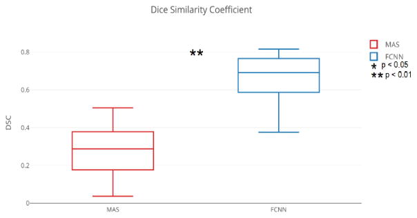
The second task was to conduct pancreas segmentation on clinical acquired T2w MR images. 138 T2 MR scans were employed to evaluate the pancreas segmentation performance. From the results, the FCNN resulted in a median DSC of 0.691 in pancreases versus 0.287 for multi-atlas.

2. METHODS

An experienced rater manually labeled the abdominal organs on a set of forty-five T2w MRI’s using MITK [14]. A radiologist labeled 138 pancreases on separate T2w MRI’s with fat suppression. In the former set, the scans were of patients with splenomegaly, and some scans were rescans performed on the same patient either twelve or twenty-four weeks after the baseline scan. The MRI’s were highly variable in both number of slices and pixel resolutions, with each view having anywhere from 47 to 512 slices and the pixel resolution falling between 0.6641 × 0.6641 × 5 mm and 1.25 × 1.25 × 8.8 mm. All of the MRI’s in the pancreas set have a pixel resolution of 1.5 × 1.5 × 5.0 mm, thirty slices on the axial view, and 256 slices on the sagittal and coronal views. Half of the scans were of patients with normal pancreases, and the other half were of patients with type 1 diabetes. The scans were captured on a Philips 3T Achieva MR Scanner. Both sets were divided into two groups, train (n = 111) and test (n = 27), which were used to train and test the accuracy of the FCNN, respectively. The FCNN was evaluated by comparing the output to the manual labels and calculating the Dice similarity coefficient (DSC).

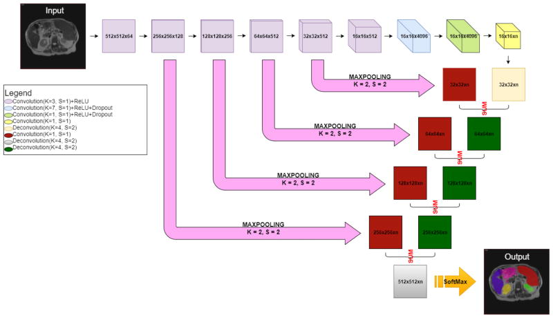
Before training the FCNN, anisotropic scans were converted to 2D images of all three views (sagittal, coronal, and axial). Following [1], the 2D images from all views were used during the training process. Using TensorFlow 0.12, we trained the FCNN with those matrices. The FCNN produces output that is the same size and contains the same number of classes (the same number of labels) as the input image. The FCNN consisted of three major portions: (1) encoder, (2) decoder, and (3) skip connection layers (Figure 2).

Figure 2.

The structure of the FCNN. The encoder is shown as the top row, where the resolution and number of channels of the output feature maps for each convolutional layer are shown in each box. For instance, the “512 × 512 × 64” means the resolution is 512 × 512 and the number of channels is 64. Then the decoder units performed the deconvolutional operations to expand the feature maps from 16 × 16 resolution to 512 × 512 resolution. To propagate the spatial information of the feature maps, the skip connection layers performed the convolutional operations to convert the number of the channels to two. The convolved feature maps were added with the deconvolved feature maps from the decoder. Finally, we derived the predications with the same size as the input image. “n” is the number of output channels (number of organs + background). The ReLU activate function was used in the activation layers. The dropout layers were used to alleviate the overfitting issue. The 2D cross-entropy loss was used as the loss function. The output hard segmentations were derived from channel number with maximum intensities on the heatmaps after the softmax layers. Specifically, our FCNN is structurally identical to the one used in [1].

Figure 2 presents the FCNN network for the multi-organ segmentation, which is a classical design with the (1) encoding, (2) decoding, and (3) skip connection. First, the encoding part consisted of the convolutional layers, which learned the features from the training images on a coarse to fine strategy. Second, the decoding part consisted of the deconvolutional layers to rescale the feature maps to the original image size. Third, the skip connection part transferred the spatial information from the encoding part to the decoding part, which enabled the decoding layers to learn both the global and local features. Finally, we derive the predication maps with the same size as the input image.

The FCNN network of pancreas segmentation is exactly the same network as Figure 2 except the number of channels is one in the skip and deconvolutions layers.

3. EXPERIMENTS

We compare our proposed method of organ segmentation using a FCNN to a naïve multi-atlas segmentation method. Both methods were evaluated against manual labels.

3.1 Organ Segmentation Using a Fully Convolutional Neural Network

First, an experienced rater labeled the liver, kidneys, stomach, and spleen of forty-five T2w MRI’s of patients who had splenomegaly. Then, the labeled MRI’s were converted from various resolutions to 512 × 512 × 512 voxels (typical voxel size = 0.78 × 0.78 × 0.59 mm). Of the dataset containing the labeled liver, kidneys, stomach, and spleen (which will hereafter be referred to as the spleen dataset), nine of the scans, excluding the scan-rescans, were randomly selected as a testing set. The remaining scans became the training set. We then trained the FCNN described in §2 with a learning rate of 0.00001. The number of output channels is six.

In pancreas segmentation, a separate set of 138 pancreas T2w MR volumes (with fat suppression) and the corresponding labels were resampled to 512 × 512 × 512 voxels (typical voxel size = 0.75 × 0.78 × 0.59 mm). Likewise, twenty-seven scans of the dataset containing the labeled pancreases (which will now be called the pancreas dataset) were also randomly chosen as a testing set, and the rest were used as a training set. We then trained the FCNN described in §2 with a learning rate of 0.00001. The number of output channels is two.

3.2 Organ Segmentation Using Naïve Multi-Atlas Method

We used naïve multi-atlas segmentation (MAS) as the baseline comparison: (1) We first performed affine transformation on all atlases to a target image, (2) then we used non-rigid registration on all registered atlases in the first step to the target image, and (3) finally we applied fusion on all transformed labels in the second step to get a final label. The generated label was compared with the corresponding manual label. The linear transformation tool we used was Dense Displacement Sampling (deeds)’s linearBCV [15–18]. The non-registration tool we used was deeds’ WBIRLCC based on a cross-correlation metric [16, 17], and we used PICSL joint label fusion tool (JLF) to fuse labels [18]. For computation efficiency, we downsampled both datasets (after already having been upsampled) by a factor of 2 to 256 × 256 × 256. For the pancreas dataset MAS, we randomly selected thirty images as atlases from the FCNN train set and performed the same MAS on the FCNN’s test set. For the spleen dataset MAS, we randomly chose fifteen images as atlases from the corresponding FCNN train set and tested them on nine images from the FCNN test set. Except WBIRLCC’s regularization value (we empirically set it as 100), we used default parameters on all three softwares.

4. RESULTS

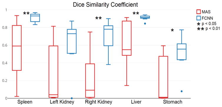
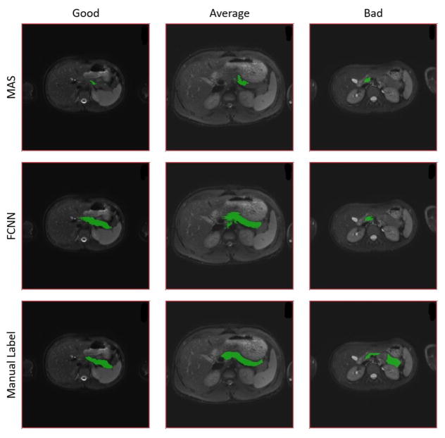
Figures 3 and 4 compare the results for the highest-performing epoch (epoch seven in total ten epochs) of the experiments involving the FCNN and MAS. Figures 5 and 6 present qualitative results. The median DSC for abdominal organ segmentation with the FCNN exceeded that of MAS by at least 0.340 for every organ tested. When considering organs that are smaller and tend to be more variable, such as the kidneys, stomach, and pancreas, this difference is even more pronounced. The difference between the two median DSC’s for the left kidney is 0.690. The FCNN obtained the best results for the multi-organ dataset in the seventh epoch while the fourth epoch produced the highest DSC for the pancreas dataset.

Figure 3.

The median DSC for abdominal organ segmentation using the FCNN is higher than that of MAS. Also, the FCNN method produces significantly better (Wilcoxon rank-sum) results than MAS for every organ except the left kidney. The results for the seventh epoch are shown.

Figure 4.

The FCNN outperforms the MAS on segmenting the pancreas on the fourth epoch. The “*” and “**” indicates the differences between FCNN and MAS are significant using a Wilcoxon signed rank test for p<0.05 and p<0.01, respectively.

Figure 5.

The qualitative results of MAS, FCNN and manual label on spleen dataset. Each color correspondents to a particular organ. Columns “Good”, “Average” and “Bad” are three subjects that from the highest, median and lowest DSC from the FCNN method.

Figure 6.

The qualitative results of MAS, FCNN and manual label on pancreas dataset. The colored regions are the pancreas segmentation. Columns “Good”, “Average” and “Bad” are three subjects that from the highest, median and lowest DSC from the FCNN method.

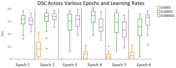
Although pancreas segmentation using our FCNN yields the best results at the fourth epoch with a learning rate of 0.00001, it also generates good results across multiple epochs and learning rates (Figure 7). When the FCNN is trained with a learning rate of 0.00001 or 0.000001, the minimum median DSC in six epochs is just 0.461. However, most are in the range of 0.6 to 0.7. On the other hand, when the FCNN is trained with a learning rate of 0.0001, the output data is poor, with a maximum DSC of 0.162 across six epochs.

Figure 7.

For the pancreas dataset, training the FCNN with a smaller learning rate produces comparable results among six epochs but functions poorly at a larger learning rate.

5. CONCLUSION AND DISCUSSION

We conclude that a FCNN can be adapted from CT applications to be used to accurately segment abdominal organs in T2w MRI’s without specific customization of the network or extensive training data. The FCNN reached a median DSC of 0.691 in pancreases, 0.930 in spleens, 0.730 in left kidneys, 0.780 in right kidneys, 0.913 in livers, and 0.556 in stomachs, all but one of which are significantly better than those of the naïve MAS. In the case of the left kidney, the MAS produced slightly better (ΔDSC < 0.08) results than the FCNN method in three cases, but the FCNN produced much better (ΔDSC > 0.16) results in the remaining cases. As a result of those three cases, the FCNN method did not perform significantly better than MAS for the left kidney.

While abdominal organ segmentation using a FCNN has proven to be a viable option, it has its own limitations: most notably, training time and large data sets. FCNN’s can require several days to train, consuming extensive GPU time, and their training sets can take months to manually label. The proposed method could be used to segment other organs within the abdomen. Another challenging issue in FCNN is the parameter tuning of the hyper parameters. The researchers typically need to carefully search the proper combinations of parameters to achieve good performance. This procedure is typically time consuming and relies on the experiences. Therefore, the method could be further refined with research defining the optimum learning rate and epoch number for a given organ or group of organs.

References

- 1.Zhou X, Takayama R, Wang S, et al. Automated segmentation of 3D anatomical structures on CT images by using a deep convolutional network based on end-to-end learning approach. 1013324-1013324-6. [Google Scholar]
- 2.Prassopoulos P, Daskalogiannaki M, Raissaki M, et al. Determination of normal splenic volume on computed tomography in relation to age, gender and body habitus. Eur Radiol. 1997;7(2):246–8. doi: 10.1007/s003300050145. [DOI] [PubMed] [Google Scholar]
- 3.Bezerra AS, D’Ippolito G, Faintuch S, et al. Determination of splenomegaly by CT: is there a place for a single measurement? AJR Am J Roentgenol. 2005;184(5):1510–3. doi: 10.2214/ajr.184.5.01841510. [DOI] [PubMed] [Google Scholar]
- 4.Linguraru MG, Sandberg JK, Jones EC, et al. Assessing splenomegaly: automated volumetric analysis of the spleen. Acad Radiol. 2013;20(6):675–84. doi: 10.1016/j.acra.2013.01.011. [DOI] [PMC free article] [PubMed] [Google Scholar]
- 5.Liu J, Huo Y, Xu Z, et al. Multi-Atlas Spleen Segmentation on CT Using Adaptive Context Learning. doi: 10.1117/12.2254437. 1013309-1013309-7. [DOI] [PMC free article] [PubMed] [Google Scholar]
- 6.Xu Z, Burke RP, Lee CP, et al. Efficient multi-atlas abdominal segmentation on clinically acquired CT with SIMPLE context learning. Medical image analysis. 2015;24(1):18–27. doi: 10.1016/j.media.2015.05.009. [DOI] [PMC free article] [PubMed] [Google Scholar]
- 7.Yetter EM, Acosta KB, Olson MC, et al. Estimating splenic volume: sonographic measurements correlated with helical CT determination. American Journal of Roentgenology. 2003;181(6):1615–1620. doi: 10.2214/ajr.181.6.1811615. [DOI] [PubMed] [Google Scholar]
- 8.Lamb P, Lund A, Kanagasabay R, et al. Spleen size: how well do linear ultrasound measurements correlate with three-dimensional CT volume assessments? The British journal of radiology. 2002;75(895):573–577. doi: 10.1259/bjr.75.895.750573. [DOI] [PubMed] [Google Scholar]
- 9.Huo Y, Liu J, Xu Z, et al. Multi-atlas Segmentation Enables Robust Multi-contrast MRI Spleen Segmentation for Splenomegaly. doi: 10.1117/12.2254147. 101330A-101330A-8. [DOI] [PMC free article] [PubMed] [Google Scholar]
- 10.Huo Y, Liu J, Xu Z, et al. Robust Multi-contrast MRI Spleen Segmentation for Splenomegaly using Multi-atlas Segmentation. IEEE Transactions on Biomedical Engineering. 2017 doi: 10.1117/12.2254147. [DOI] [PMC free article] [PubMed] [Google Scholar]
- 11.Xu Z, Gertz AL, Burke RP, et al. Improving Spleen Volume Estimation Via Computer-assisted Segmentation on Clinically Acquired CT Scans. Academic radiology. 2016;23(10):1214–1220. doi: 10.1016/j.acra.2016.05.015. [DOI] [PMC free article] [PubMed] [Google Scholar]
- 12.LeCun Y, Bengio Y, Hinton G. Deep learning. Nature. 2015;521(7553):436–444. doi: 10.1038/nature14539. [DOI] [PubMed] [Google Scholar]
- 13.Long J, Shelhamer E, Darrell T. Fully convolutional networks for semantic segmentation. :3431–3440. doi: 10.1109/TPAMI.2016.2572683. [DOI] [PubMed] [Google Scholar]
- 14.Wolf I, Vetter M, Wegner I, et al. The medical imaging interaction toolkit. Medical image analysis. 2005;9(6):594–604. doi: 10.1016/j.media.2005.04.005. [DOI] [PubMed] [Google Scholar]
- 15.Heinrich MP, Jenkinson M, Brady M, et al. MRF-based deformable registration and ventilation estimation of lung CT. IEEE transactions on medical imaging. 2013;32(7):1239–1248. doi: 10.1109/TMI.2013.2246577. [DOI] [PubMed] [Google Scholar]
- 16.Heinrich MP, Jenkinson M, Papież BW, et al. Towards realtime multimodal fusion for image-guided interventions using self-similarities. :187–194. doi: 10.1007/978-3-642-40811-3_24. [DOI] [PubMed] [Google Scholar]
- 17.Heinrich MP, Papież BW, Schnabel JA, et al. Non-parametric discrete registration with convex optimisation. :51–61. [Google Scholar]
- 18.Wang H, Yushkevich PA. Multi-atlas segmentation with joint label fusion and corrective learning—an open source implementation. Frontiers in neuroinformatics. 2013;7 doi: 10.3389/fninf.2013.00027. [DOI] [PMC free article] [PubMed] [Google Scholar]