When tractography meets tracer injections: a systematic study of trends and variation sources of diffusion-based connectivity

Abstract

Tractography is a powerful technique capable of non-invasively reconstructing the structural connections in the brain using diffusion MRI images, but the validation of tractograms is challenging due to lack of ground truth. Owing to recent developments in mapping the mouse brain connectome, high resolution tracer injection based axonal projection maps have been created and quickly adopted for the validation of tractography. Previous studies using tracer injections mainly focused on investigating the match in projections and optimal tractography protocols. Being a complicated technique however, tractography relies on multiple stages of operations and parameters. These factors introduce large variabilities in tractograms, hindering the optimization of protocols and making the interpretation of results difficult. Based on this observation, in contrast to previous studies, in this work we focused on quantifying and ranking the amount of performance variation introduced by these factors. For this purpose, we performed over a million tractography experiments and studied the variability across different subjects, injections, anatomical constraints and tractography parameters. By using N-way ANOVA analysis we show that all tractography parameters are significant and importantly performance variations with respect to the differences in subjects is comparable to the variations due to tractography parameters, which strongly underlines the importance of fully documenting the tractography protocols in scientific experiments. We also quantitatively show that inclusion of anatomical constraints is the most significant factor for improving tractography performance. Although this critical factor helps reduce false positives, our analysis indicates that anatomy-informed tractography still fails to capture a large portion of axonal projections.

1. Introduction

Tractography is an important and unique tool for the non-invasive, in vivo study of brain connections (Mori et al. 1999; Basser et al. 2000). With the emergence of modern and comprehensive diffusion MRI (dMRI) acquisition protocols, we can now map the human brain connections at an unprecedented resolution (Wandell 2016). Particularly, as a result of the advances in multi-band and parallel imaging technologies (Feinberg et al. 2010; Moeller et al. 2010; Setsompop et al. 2012) and their successful application in the Human Connectome Project (HCP) (Toga et al. 2012; Van Essen et al. 2013), there have been substantial progress in multi-shell dMRI data acquisition and fiber orientation modeling (Yeh et al. 2010; Jbabdi et al. 2012; Jeurissen et al. 2014; Cheng et al. 2014). With the latest efforts on studying tissue microstructure and compartment modeling (Panagiotaki et al. 2012; Ferizi et al. 2014; Novikov et al. 2016; Tran and Shi 2015) that provide even more accurate local uncertainty models for fiber orientation densities (FODs), the community has been improving tractography algorithms as well (Aydogan and Shi 2016; Reisert et al. 2014), paving the way towards quantitative tractograms (Jbabdi and Johansen-Berg 2011; Girard et al. 2014).

In spite of the developments in dMRI and tractography techniques, we still face the long standing challenge of missing ground truth for the validation of connections reconstructed by tractography. Validations using phantoms (Leemans et al. 2005; Campbell et al. 2006; Fieremans et al. 2008; Pullens et al. 2010; Bach et al. 2014; Girard et al. 2014; Neher et al. 2014) were proposed in various previous studies, but it is unclear how results obtained for artificial phantoms translate to biological tissues, especially when considering the neuroanatomical complexity of living organisms. Anatomically and histologically, tracer injections have long been considered the gold standard for the validation of tractography. While this usually is challenging, many important studies were done to compare tractography with tracer injections. Including on post-mortem human brains (Seehaus et al. 2012), tracer injection based validations were done on monkeys (Dauguet et al. 2007; Schmahmann et al. 2007; Jbabdi et al. 2013; Donahue et al. 2016), pigs (Dyrby et al. 2007; Knösche et al. 2015) and rats (Gyengesi et al. 2014). Notably, mapping the mouse brain connectome has seen tremendous progress in creating detailed axonal projection maps with whole brain coverage (Zingg et al. 2014; Oh et al. 2014). The mouse brain connectome from the Allen Mouse Brain Atlas (AMBA) (Oh et al. 2014) quickly became an important resource for validating the connectivity constructed by diffusion imaging (Keifer et al. 2015; Calabrese et al. 2015; Chen et al. 2015b).

Previous validation studies show that obtaining connections in the brain using dMRI based tractography is a challenging problem. Differences across image acquisition techniques (Tuch et al. 2002; Wedeen et al. 2005; Feinberg et al. 2010; Aganj et al. 2010; Setsompop et al. 2012; Moeller et al. 2010), diffusion models (Tournier et al. 2004; Tuch 2004; Panagiotaki et al. 2012; Basser et al. 1994), tractography algorithms and parameters (Fillard et al. 2011; Mangin et al. 2013; Pestilli et al. 2014; Daducci et al. 2015; Smith et al. 2015) all introduce limits and assumptions that result in biases and variability, affecting the accuracy, reliability and reproducibility (Besseling et al. 2012; Girard et al. 2014; Thomas et al. 2014).

Without carefully validating the connections and studying the factors that affect the performance of our complicated techniques, it is difficult to fully leverage the rich information obtained by tractography. A quantitative insight on the sources of performance variation is therefore crucial to improve how we conduct tractography experiments and interpret the results. Consequently, it is critical to rigorously analyze and study these factors which is a challenging and multidimensional problem.

Many validation studies addressing a single or few dimensions of the sources of variations have been published earlier to improve the practices in tractography. In (Thomas et al. 2014), projections obtained using anterograde tracer injections from two locations of a macaque brain were compared against the tractography results obtained from the same subject. Authors compared the variability between deterministic and probabilistic tractography results across four different diffusion models and four curvature thresholds. They reported common limitations of diffusion models and tractography techniques but did not quantitatively analyze and rank how much each factor influence the results. (Gyengesi et al. 2014) compared the variability in performance with respect to different tractography techniques on twelve fiber bundles in rat brains and reported limitations and advantages of deterministic and probabilistic approaches. (Chen et al. 2015c) used a single mouse brain and studied the variation in probabilistic tractography results with respect to the variation in fractional anisotropy (FA) and curvature thresholds. Authors suggested optimal parameters by testing three different FA and five different curvature thresholds. In (Seehaus et al. 2012), carbocyanine dyes were used as tracers on a human post-mortem tractography validation experiment. The variability of results was studied using three seed locations and nine different FA thresholds. Authors reported that for their study FA values between 0.02 and 0.08 were optimal. In (Dauguet et al. 2007), tractography results were compared with 3D histological tracing of two injections on pre- and post-central gyrus on a single macaque brain. The variability in results with respect to FA, curvature and step size were studied. Authors tested 13 different FA, 11 different curvature and 13 different step size values. However, they fixed the other two parameters while checking the variability due to a single parameter, thus did not address the coupling effects of multiple parameters.

Despite its relatively long history, tractography lacks maturity. Previous validation works show that the large number of sources for variation plays an important role, obstructing the way for the clinical applications of this unique technique. With such vast options for streamline reconstruction, there are very few common practices adapted in the literature, leaving a plethora of ways for not adopting adequate experimental protocols. This in addition makes parameter optimization studies challenging since the significance of optimal parameters is questionable when several other variation sources are in effect. Due to the large variability in scanners, pre-processing pipelines, diffusion models and tractography algorithms, inevitably optimal parameters for tractography parameters also vary. Owing to this reason, in contrast to previous validation studies, we chose to focus on the extent of variability due to several parameters. Instead of presenting optimal values, our study provides systematic ways to obtain robust and reproducible results with tractography. While meticulously inspecting the trends, we not only take into account the coupled effects of several parameters, but we also rank how much variability each source introduces.

Our aim with this work is to expand our understanding on how to better conduct tractography experiments and interpret results by taking into account the sources of variations. For that we present results from our extensive (over 1 million) multidimensional tractography validation experiments using multi-shell dMRI data from mouse brains and tracer injections from AMBA. We studied the variability in the results with respect to seven different factors including their cross relations with each other using N-way ANOVA analysis. The factors we studied are: subject, tractography parameters (step size, curvature, cut-off, number of streamlines), use of anatomical constraints and the fiber bundle that is studied.

Our results have significant implications. Firstly and most importantly, we show that the variations in tractograms with respect to differences in subjects is comparable to variations with respect to tractography parameters used in the experiments. Secondly, we show that the tractography results significantly vary with respect to all parameters, including the commonly overlooked step size and number of streamlines. Lastly, our experiments show that while incorporating prior anatomical knowledge can dramatically reduce false positives, the overlaps between tractograms and injection experiments are still not ideal due to false negatives.

2. Materials and Methods

2.1. Materials

Eight wild-type female mice (mus musculus) aged eight to ten weeks old were used as subjects. Subjects were deeply anesthetized with isoflurane gas then transcardially perfused with phosphate buffered saline (PBS) with 0.05% heparin pH 7.4 at 37°C followed by 4% paraformaldehyde in PBS pH 7.4 at 37°C to fix tissue. The subjects were then rapidly decapitated and skin, muscle, and bottom jaw were removed from the skull. The mouse brains intact within the skull were immediately postfixed in 4% paraformaldehyde in PBS pH 7.4 at 4°C overnight. The following day the mouse brains were transferred to storage buffer, PBS pH 7.4 with 0.01% sodium azide and kept at 4°C. The mouse brains were transferred to fresh storage buffer four more times during the first forty-eight hours after fixation, and then transferred to fresh storage buffer and rocked on a nutating rotator for five days at 4°C to remove any remaining paraformaldehyde. Finally the mouse brains were transferred to fresh storage buffer and shipped from the Dulawa Lab then at the University of Chicago to the California Institute of Technology on ice for MRI data collection. All procedures involving animals were done in accordance with the ethical standards of the institution.

2.2. Multi-shell imaging of mouse brains

Fixed mouse brains intact within the skull were soaked in 5mM Prohance® (Bracco Diagnostics, Inc., NJ) for 3 days prior to imaging to decrease overall T1 relaxation rates. They were then scanned three at a time immersed in Galden® (Solvay Solexis, Inc., NJ) with a 7 Tesla Bruker BioSpin MRI scanner at the California Institute of Technology. Diffusion weighted images (DWI) were acquired using a 4 segment 3D spin-echo echo-planar imaging (SE-EPI) sequence: 128×110×100 matrix; voxel size: 0.2×0.2×0.2 mm³, TE=50 ms; TR=1000 ms, δ=9 ms, Δ=13 ms, bandwidth=303 kHz, double sampling, NA=1, yielding scan time ~10 hr. (When scaled to the size of an average human brain (Nolte 2009), the imaging resolution corresponds to an isotropic 2.7mm which is well within the range of typical human dMRI acquisition settings.) 93 separate volumes were acquired: 3 T2-weighted volumes (voxel size: 0.1×0.1×0.1 mm³) with no diffusion sensitization (B0 image) and 90 diffusion-weighted images. DWIs were acquired with different angular samplings across 3 distinct b-value shells: 1000, 3000 and 5000 s/mm² (each b-value shell contained 30 diffusion-weighted images), where the gradient directions were generated with optimal distribution across the spheres (Caruyer et al. 2013).

2.3. Allen Mouse Brain Atlas and selection of injection locations

The Allen Mouse Brain Atlas (AMBA) provides detailed tracer injection and projection density images from a large number of sites covering the mouse brains (Oh et al. 2014). All AMBA data were saved in an atlas space with a detailed set of anatomical labels (Dong 2007). The AMBA atlas was created by registering and averaging serial two-photon microscopy (STP) images of 1231 specimens (Kuan et al. 2015). AMBA provides 10μm, 25μm, 50μm and 100μm resolution versions of the atlas. In our study we used the 25μm resolution images because they provide a good balance between the level of detail and memory required for computation. All data from the AMBA are distributed in the NRRD format and uses the Common Coordinate Framework (CCF) (Oh et al. 2014). In order to utilize conventional neuroimaging tools, we wrote a custom script to convert the AMBA data into RAS orientation and saved them in the NIFTI format. As of June 2017, there are 2546 anterograde recombinant adeno-associated virus (rAAV) tracer studies shared by the AMBA. Tracer studies were done on transgenic mouse lines as well as wild-types. Due to the heavy computational load in our validation experiments, we limited our study to ten injection sites that were done on wild-type mice. These ten injections were selected from different parts of the brain in order to cover a large variety of projections. The injection IDs used in this article, original injection IDs (given by the AMBA), and their anatomical locations are listed in Table 1. 3D visualizations of the injection sites and their projections are shown in Fig. 1.

Table 1.

List of injection IDs and anatomical locations used in the study

Injection ID	Original injection ID	Injection Location
I1	100142569	Anteroventral nucleus of thalamus
I2	113887868	Primary visual area
I3	114249084	Cortical amygdalar area
I4	114290938	Primary somatosensory area, mouth
I5	180435652	Ectorhinal area
I6	180719293	Primary motor area
I7	127255254	Nucleus accumbens
I8	309385637	Nucleus of the lateral lemniscus
I9	272737914	Gustatory area
I10	112745787	Dentate gyrus

Fig. 1.

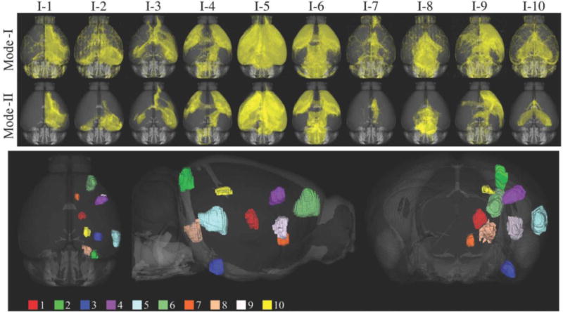
Top panel shows the 3D volume renderings for the ten tracer projection densities used in Mode-I and Mode-II comparisons. Injection sites used in the study are visualized on the bottom panel.

2.4. Pre-processing of MRI data

The skull-stripping tool (BSE) (Shattuck and Leahy 2002) of BrainSuite was used to extract masks for individual mouse brains from the T2 image. Each brain was carefully extracted by manually adjusting BSE parameters. Brain masks were then reoriented to the RAS orientation with an in-house developed software tool that uses manually annotated landmarks. Both T2 and diffusion MRI were then warped to align with AMBA using the ANTs registration tool (Avants et al. 2011). Because AMBA is prepared using STP images, we used the mutual information similarity metric for all registration steps. A comparison using a checkerboard pattern between AMBA and a registered image is shown on an axial slice in Fig. 2 (a). For each subject, registration error is quantitatively measured using the average displacement of manually marked landmarks on the AMBA and subject’s T2 image. For that, we used the landmarks proposed in (Sergejeva et al. 2015). In this study 16 landmarks are recommended for the C57BL/6J mouse brain MRI registration: 2 landmarks are in cerebellum, 1 in middle cortex, 1 in periaqueductal gray, 1 in pontine nucleus, 1 in hippocampus, 3 in interpeduncular nucleus, 1 in corpus callosum, 1 in middle ventricle, 2 in anterior commissure and 3 in frontal areas. Among the 16 landmarks, we did not use the 2 in cerebellum since dorsal sections of AMBA do not include these regions. In our dataset, the mean and standard deviation of average displacement of all subjects are measured to be 145.35±29.37μm which corresponds to 1.45±0.3 voxels in MRI space. This error is comparable to that obtained by (Sergejeva et al. 2015) which was 134±20μm (1.54±0.23 voxels). The nonlinear transforms were saved and used to warp the injection sites and tracer projection density maps of the AMBA to individual mouse brains for our tractography experiments. Additionally, FSL’s eddy_correct tool is used to reduce the artifacts in dMRI due to Eddy currents (Jenkinson et al. 2012).

Fig. 2.

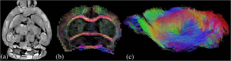
(a) Visualization for registration accuracy using a checkerboard pattern on an axial slice (b) FODs reconstructed from multi-shell mouse brain dMRI data are plotted on a coronal slice (c) Whole brain tractography results from FOD-based probabilistic tractography

2.5. FOD Reconstruction from multi-shell diffusion MRI

Using the multi-shell diffusion MRI (dMRI) data of mouse brains, we applied the novel reconstruction method we developed recently in (Tran and Shi 2015; Kammen et al. 2016) to compute FODs that are used in our tractography experiments. At each voxel, the FOD is a scalar function defined on the unit sphere that represents the probability of streamlines in each direction (Fig. 2 (b)). Numerically each FOD is represented with spherical harmonics up to the order of 12 that matches the number of gradient directions in our acquisition protocol. For the diffusivity of the stick kernel in our computational framework, we used 0.0008 mm²/s following previous literature on post-mortem mouse brain diffusion imaging (Wu et al. 2013; Wu et al. 2014). Note that this is smaller than the kernel diffusivity that we typically use for in vivo human brain imaging data from the HCP. Using FOD-based tractography, we can visualize the connectivity of mouse brains (Fig. 2 (c)) and study its relation to the underlying anatomy.

2.6. Tractography technique and parameter values

We used the iFOD2 algorithm of the MRtrix3 software (Tournier et al. 2010; Tournier et al. 2012) for FOD-based probabilistic tractography. Injection density images from the AMBA were registered to each mouse brain image and used as seed regions for tractography. Because injection density images provide a probability density function for the injected tracer, we used the –seed_rejection flag of tckgen command of MRtrix3. This option generates track seeds proportional to the tracer density at each voxel. To thoroughly investigate the impact of tracking parameters, we used nine different values for the following parameters in tractography: step, curvature and cut-off (FOD amplitude threshold for terminating tracks). Other tractography parameters used in the experiments were fixed as minlength = 0.1mm, maxlength = 50mm and trials = 1000. The term “curvature” is used synonymous to “radius of curvature” and values were converted to angle for the tckgen command. We also varied the number of total streamlines per each injection site with ten different values to examine the convergence of overlap with respect to this parameter. For each injection, we overall conducted 7290 (=9×9×9×10) tractography experiments.

The values of the varied tractography parameters are listed in Table 2. Because it is common to set step size as a fraction of voxel dimensions, this is also listed. Similarly, curvature is also commonly set in terms of angular deviations that we also included in the table. Notice that step size (with respect to voxel size), curvature (in angles) and number of streamlines used in the tests are within the typical ranges of tractography experiments done in the literature. Cut-off values however are different since we used post-mortem mice in our experiments which has much lower diffusivity compared to the in vivo human case.

Table 2.

Tracking parameters used in the experiments. Step and curvature are listed with two commonly used units.

Step (μm)	10	15	20	25	30	35	40	45	50
Step (×voxel size)	1/20	1/13.3	1/10	1/8	1/6.6	1/5.7	1/5	1/4.4	1/4
Curvature (μm)	35	39	44	50	59	73	97	144	287
Curvature (angle in °)*	90	80	70	60	50	40	30	20	10
Cut-off (×10−2)**	0.75	1.125	1.5	1.875	2.25	2.625	3	3.375	3.75
Number of streamlines (×103)	50	100	150	200	250	300	350	400	450	500

^*angle is computed for step size of 50μm.

^**cut-off is the FOD amplitude threshold for stopping the tracks.

2.7. Quantitative comparison of tractography and tracer injections

We used the projection density images provided by the AMBA as the ground truth. Projection density is defined as the ratio of number of projection detected pixels to number of all pixels in the division (Kuan et al. 2015), i.e.: the maximum projection density value is 1 and it indicates that all the pixels in the division are projected by the neurons from the injection area. However, the projection density values are challenging to use for quantitative analysis due to variations among intensity profiles in different sections as well as changes in experimental procedures for different injection sites such as the tracer dose. Based on these reasons, as the ground truth, instead of considering the amount of projections from an injection site to a voxel, we chose to consider whether there exists a projection to this voxel or not.

We compared the ground truth with tractography results by obtaining the voxels that have projections from the injection site. For this purpose we computed track density images (TDI) at the same resolution as AMBA (Calamante et al. 2012). TDI is obtained using the tckmap command of MRtrix3.

In order to compare tractography results with AMBA’s injection studies, we used two different modes in our analysis. Mode-I and Mode-II separately consider the two common applications of tractography. Mode-I comparison aims to measure the accuracy of tractography when used for general exploration, i.e.: identification of all tracks from a given seed region. On the other hand, Mode-II comparison aims to quantify accuracy of tractography when used for targeted exploration, i.e.: extraction of tracks from a given region to another. In Mode-I comparison, voxels inside the brain mask with non-zero projection density are considered as ‘positive condition’ otherwise they are ‘negative condition’. In Mode-II comparison, we apply constraints on both the projection density images and tractograms. For tracer projection maps, all projected voxels ideally should be morphologically connected to the injection site without any gaps. However, this is not the case in projection density images due to discretization errors and spurious projections. For Mode-II comparison, as ground truth, we used the voxels that have more than 1% projection density and form a single connected component with the injection site. Besides using the injection site as the seed ROI for tractography, we also apply this connected component as the target (include) ROI for the tractography. The use of this additional anatomical constraint in Mode-II experiments is similar to the streamline reconstruction protocols in human brain imaging, where multiple ROIs were typically used to identify the major fiber bundles. Our goal is to examine the degree of improvement that can be achieved with the incorporation of additional anatomical constraints. Streamlines for Mode-II comparisons are obtained using the ones computed for Mode-I comparisons by trimming segments from the ends of each streamline until a projection site is hit. Fig. 1 shows volume renderings of Mode-I and Mode-II projections for all the injections and Fig. 3 shows a graphical explanation for the ground truths and predictions used for Mode-I and Mode-II analysis.

Fig. 3.

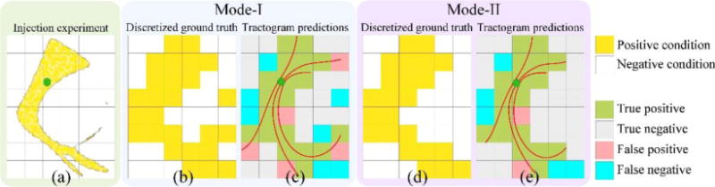
Graphical description of Mode-I and Mode-II analysis (a) Injection seed and projections are shown with green and yellow respectively (b) Mode-I uses the discretized ground that is the existence of projections to voxels (c) Mode-I results are computed using the streamlines projecting from the seed location (d) In Mode-II spurious projections are removed from the ground truth (e) Mode-II results are computed by trimming the ends of streamlines that are outside the ground truth. This presents the case where an anatomical constraint requires the end points of all streamlines to project to a ground truth voxel.

To quantitatively evaluate the performance of tractography results, we form a predicted projection label image from the TDI image and calculate the overlap with ground truth labels. To form the predicted projection label image, we mark a voxel with the true label if it has a non-zero TDI value; otherwise it is marked with the false label. Therefore, a true label indicates that we predict the existence of projections to that voxel, and a false label indicates that no projection is predicted. The ground truth label image is obtained similarly by thresholding the tracer projection density images used in either Mode-I or Mode-II comparisons. Using the predicted projection label and the ground truth label images, we compute the number of voxels belonging to true positives (TP), false positives (FP), true negatives (TN) and false negatives (FN) (Fig. 3 (c-d)). After that, the following measures were calculated to characterize the performance of tractography results: true positive rate $(\mathit{TPR}=\frac{TP}{TP+FN})$, false positive rate $(\mathit{FPR}=\frac{FP}{FP+TN})$ and DICE coefficient $(\mathit{DICE}=\frac{2\times TP}{TP+FP+TP+FN})$ (Dice 1945).

2.8. Statistical analysis of variation

We used N-way ANOVA analysis to study the sources of variation in our results. Similar to previous studies (Besseling et al. 2012; Dauguet et al. 2007), we focused on the variation in DICE measure since it is a one dimensional quantity that measures the overlap quality. By applying N-way ANOVA analysis using the DICE measure, we identified the changes in the quality of overlap between different groups as well as the variation within them. As a part of the ANOVA analysis, we computed the F-statistic to test and quantify the significance of parameters. ANOVA analysis is done using MATLAB (MathWorks 2012). We showed that our dataset satisfies the ANOVA requirements in Supplementary Material A.

3. Results

The overlap between tractography and tracer injection experiments changes dramatically with different choices of parameter combinations. Before we analyze the sources of this variation, in section 3.1, we demonstrate how the quantitative measures used in this study (TPR, FPR and DICE) visually correspond to the overlap. Here we also briefly point out the effect of subject variability on the results. In section 3.2, we extend the results of section 3.1 by varying each of the parameters separately. With this, some of the trends due to parameter variations are observable. In section 3.3, we dig deeper into the trends, by including multiple injection locations which gives a complete overview of the trends in our seven dimensional parameter space. (More detailed information and figures on the trends are provided in the supplemental materials for interested readers.) In section 3.4, we analyze the sources of trends and reveal how much each of the parameters contribute to the variation in performance.

3.1. Examination of overlap measures and variation across subjects

Fig. 4 visualizes examples for a range of TPR, FPR and DICE in order to establish a visual link between these performance measures and the overlap quality. Fig. 4 shows the 3D overlap between projection density images and tractography results for the 6^th injection site that we denote as I6. For qualitative inspection, we used 2 subjects, M1 and M2, and considered 3 different sets of parameters represented as Case A, Case B and Case C that are listed in Table 3.

Fig. 4.

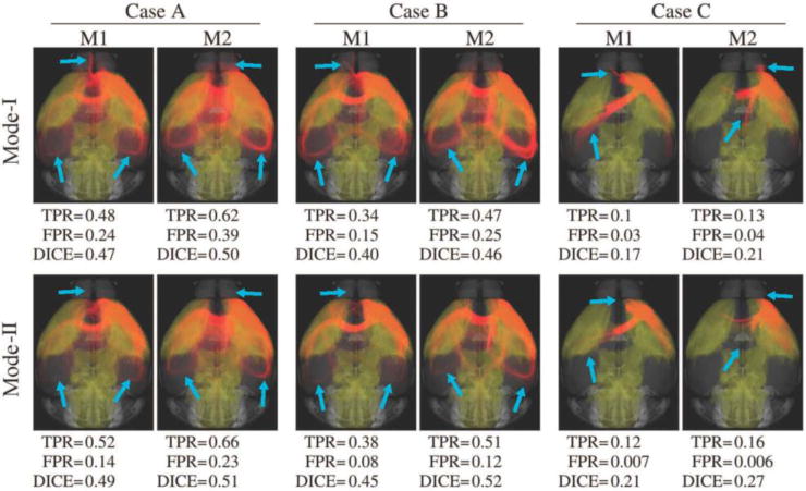
3D overlap of the tracer projection density for I6 (shown in yellow) and tractography results (shown in red) using two of the eight subjects, M1 and M2. Top and bottom rows show the results for Mode-I and Mode-II comparisons, respectively. While Mode-II does not noticeably affect the tracer data since it only removes spurious projections, there are visible differences in tractograms (shown with blue arrows) due to the introduction of anatomical constraints. Computed measures are listed under each experiment. Case A shows better results compared to Cases B and C.

Table 3.

Tracking parameters used for the qualitative examination

	Step (μm)	Curvature (μm)	Cut-off (×10−2)	Number of streamlines
Case A	50	35	1.5	500K
Case B	20	39	2.25	500K
Case C	10	287	3.75	500K

I6 projects to a large portion of the brain including somatosensory areas on both hemispheres and dorsal regions such as the medullary nuclei. We observed in our experiments that most of the parameter combinations were successful in obtaining projections to somatosensory areas. Contralateral and dorsal connections are more visible for M2. This coincides with the values of Dice coefficient which is an indicator for the quality of overlap. Capturing dorsal projections, however, required more flexible parameter combinations. Basically Case A, B and C visually show relatively good, moderate and bad agreements between the tracer projection and tractography. While differences can be observed between the results from the two mouse brains, the overall trends for Case A, B and C are consistent. Another consistent trend is the improvement of the overlap measures when the anatomical constraint was added to obtain Mode-II results. For all cases, the inclusion of prior anatomical knowledge improved the result for both subjects.

3.2. Examination of overlap variations due to tractography parameters and anatomical constraints

In order to examine the effect of tractography parameters, we used Case A, B and C shown in Table 3 as reference points and varied each of the four parameters. The results are shown in Fig. 5 as FPR vs TPR plots on the receiver operator characteristic (ROC) plane. Overall we run 204 tractography experiments for each subject. Plots in Fig. 5 can be considered as samples from ROC curves for the variation of each tractography parameter separately. The size of data points is in proportion to the corresponding Dice coefficient computed from the same experiment. The results from the reference parameters listed in Table 3 are marked with an ‘x’ for each case. Fig. 5 confirms that Mode-II results always yield better matches with the injection experiments. It is also observed that although step size changes the results, compared to other parameters its effect is not as pronounced. A large radius of curvature seems to be a strong constraint; however, decreasing it does not improve the match for very low curvature values. Decreasing the cut-off threshold value of the FOD magnitude increases the TPR but also increases the FPR. There is a big difference in overlap quality between results generated using low and high number of streamlines. Increasing the number of streamlines shows a converging pattern for all cases.

Fig. 5.

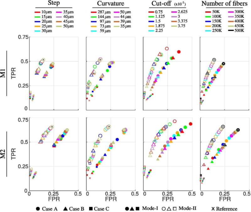
Effects of parameter variations on the overlapping measures between tractography and tracer projection density for I6. Top and bottom rows show the results for subjects M1 and M2, respectively. Reference points corresponding to Case A, B and C in Table 3 are plotted as x. On each column, only one of the parameters is varied, i.e.: for the two plots under curvature, only the curvature parameter is changed, all other parameters are kept same. The size of the data points is in proportion to the DICE coefficient.

3.3. Examination of overlap variations due to injection sites

To examine the results for different injection sites, we picked I1 and I6 for the first subject (M1). For both injection sites, we ran tractography experiments with all the possible 9×9×9×10=7290 combinations of parameter choices listed in Table 2. Because we conducted both Mode-I and Mode-II analysis, there are overall 14580 experiments for each injection. The TPR vs FPR values showing the trends with respect to the changes in number of streamlines and cutoff parameters are plotted in Fig. 6. Notice that all of the 14580 data points in columns one and three are identical for each row, i.e.: for each injection site. However they are plotted in different coloring schemes in order to highlight the trends with respect to changes in number of streamlines (first column) and cut-off (third column) parameters. Similarly the data points used in second and forth columns are identical. Second column shows a sub-set of the data points where the cut-off value is fixed to 0.75×10⁻² in order to further clarify the trend with respect to changes in number of the streamlines. Similarly in the fourth column, number of streamlines is fixed to 500K which better exposes the trend due to cut-off variation.

Fig. 6.

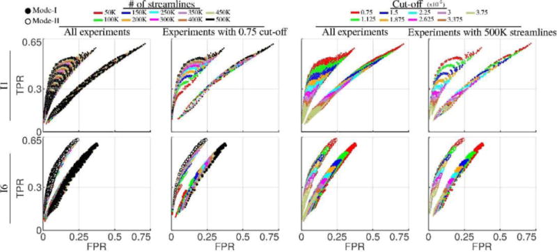
Variability of tractography performances with respect to number of streamlines and cut-off parameters. The dimensions of data points are in proportion to the DICE coefficients. First and third rows show the same data points which are collected from all of the experiments using injections I1 and I6 on M1 (14580 experiments = 2 modes × 9 step sizes × 9 curvatures × 9 cut-off thresholds × 10 number of streamlines). However the coloring of points are done with respect to number of streamlines in the first column and cut-off in the third to highlight the trends. Cut-off is fixed to 0.75×10⁻² in the second column to clarify the trend with respect to changes in number of streamlines. Similarly in the fourth column number of streamlines is fixed to 500K to emphasize the trend with respect to cut-off changes.

Overall we can see quite dramatic differences between the plots for I1 and I6. This shows that anatomy plays a key role in determining the performance of tractography experiments in terms of the TPR, FPR and DICE values. It is also consistent with the previous experiments where Mode-II analysis generated higher agreements between tractography and tracer projection density images. From Fig. 6, we can see the data points with different cut-off thresholds are stratified into distinguished bands. Experiments with high cut-off thresholds yield lower TPR, FPR and DICE values. Relaxing this constraint enables us to obtain higher TPR at the cost of higher FPR. On the other hand, the results in Fig. 6 show that the number of streamlines does not have a similar effect on constraining the performance of the tractography experiments. It can be observed that both TPR and FPR values improve almost monotonically with the increase of number of streamlines. Given this observation, we selected the data points with the number of streamlines at the maximum value (500K) and plotted them separately by coloring them according to the cut-off values. These plots more clearly illustrate the effect of the cut-off values on the performance of tractography. With the change of the cut-off thresholds, we can see a wide range of overlapping measures.

To illustrate the effects of the other two parameters: curvature and step, we plotted in Fig. 7 the data points with the maximum number of streamlines (500K) and three representative cut-off thresholds, low cut-off (0.75×10⁻²), medium cut-off (2.25×10⁻²) and high cut-off (3.75×10⁻²) . In order to have a clearer visualization, we only used data points from four representative curvature and step values. For the visualization of the plots, we used different symbols to indicate different curvature values and we used different colors to indicate different step sizes. Similar to the cut-off parameter, curvature imposes a strong constraint and in general high curvature values yield low TPR and FPR. Relaxing curvature by decreasing its value increases both TPR and FPR. On the other hand, decreasing the step size has an opposite effect. Smaller step sizes in general yield lower TPR and FPR.

Fig. 7.

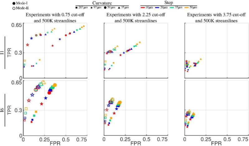
Variability of tractography performances with respect to curvature and step size parameters. The dimensions of data points are in proportion to the DICE coefficients. All data points are a sub-set of the experiments shown in Fig. 6. In order to keep the plots simple, the number of streamlines is fixed to 500K and three different (fixed) cut-off values are shown in each column. Data points with respect to varying curvature values are shown with different symbols whereas different colors are used to show the points for varying step size.

More details on the overall overlap variation due to tractography parameters, anatomical constraints are given on Supplementary Material B. Also in Supplementary Material C, detailed figures are provided on the overall impact of injection sites, mouse brains, and tractography parameters.

3.4. ANOVA analysis and the ranking of variation sources

In the previous sections, we examined several factors that affect the performance of tractography results. In this part, we perform N-way ANOVA analysis in order to compare the effects of these factors. Top panel of Fig. 8 shows the individual group means plotted using MATLAB’s multcompare command. By checking the means and confidence intervals, we determined that only groups with curvature=287μm are significantly different from all others and have a low mean value that is not close to other groups. We marked this data point as an outlier, crossed it with dark green and removed it from further analysis. (Outlier removal is explained in more detail in Supplementary Material D.) Gray and black in Fig. 8 show ANOVA results before and after outlier removal respectively. Red data points show results when Mode-I and Mode-II are separated. Fig. 8 shows that Mode-II gives higher DICE coefficients for all groups. Decreasing step or curvature increases the quality of overlap for Mode-II, however, this trend is opposite for Mode-I. For both modes, decreasing the cut-off threshold increases the DICE values. There is not a significant gain below cutoff=0.015 for Mode-II.

Fig. 8.

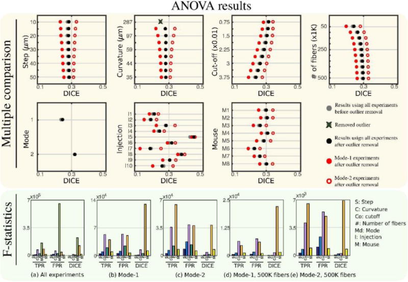
Multiple comparison plots and F-statistics obtained by N-way ANOVA analysis. Multiple comparison shows a large separation of results with respect to mode. Red data points on multiple comparison plots show ANOVA results obtained when modes are separated. The outlier curvature=287 μm group is removed from all F-statistic results.

In the lower panel of Fig. 8, (a) shows the F-statistics belonging to each variation source using all the experiments after the outlier group is removed. All groups are found to be statistically significant (p ≪ 0.05). Here we also included the results for TPR and FPR. Analysis mode is determined to be the most significant parameter for all measures. The order of significance between the other parameters change depending on the measure. For DICE coefficient, tractography parameters contribute to the total variation less than the injection or the subject for most cases.

Our results show that both the injection and the subject used in the experiments are big contributors to the total variation of the quality of overlap and they are significant. Especially, when Mode-I and Mode-II are separated, their significance becomes clearer, Fig. 8 (b, c). For DICE coefficient injection is the most significant source of variation when modes are separated. We observe from Fig. 8 (a, b and c) that, for most cases, number of streamlines is a more significant parameter than both step and curvature. Fig. 8 (d) shows that most of the variation from number of streamlines is due to low values and the variation decreases with the increase in the number of streamlines. We find it interesting to determine the sources of variation in the case that the experiments are performed with a large enough number of streamlines. Fig. 8 (d, e) show F-statistics when modes are separated and the largest number of streamlines are used. We observe that, in this case the two most significant sources of variation in the quality of overlap are the injection location and the subject either of which are parameters used to compute the tracks. The most significant tractography parameter is the cut-off threshold which is followed by curvature and step.

4. Discussion

Understanding the roots of performance variation in tractograms is important to advance our techniques towards more reliable and reproducible results which are essential for clinical practices. It is well known from earlier studies that due to several factors including subject (Heiervang et al. 2006; Willats et al. 2014), tractography parameters (Mangin et al. 2013; Yeh et al. 2016; Thomas et al. 2014; Azadbakht et al. 2015), anatomical constraints and the fiber system (Smith et al. 2012; Donahue et al. 2016), performance of tractography varies. Although, sources for variability that are studied in this work are well-known, how much they contribute to variability has not been thoroughly studied. Learning more about this information is critical in (i) setting up protocols for tractography and (ii) interpreting results. However, studying the coupled effects of factors is challenging due to the big dimension of affecting parameters. This demands a large set of experiments to be performed to cover a sufficient subset of the whole parameter space. For the validation of tractography, this is an additional challenge on top of the lack of ground truth, which we tried to overcome in this work.

For our study, we sampled a large portion of the parameter space responsible for performance variations in tractography, extracted trends and attained a comprehensive understanding of the factors within practical ranges of parameter choices. We collected results from 1,166,400 experiments: 8 mouse brains × 10 injections × 2 modes of analysis × 9 step sizes × 9 curvatures × 9 cut-off thresholds × 10 number of streamlines. It took about 40 days to complete all tractography experiments using 350 nodes in our computer cluster. The compressed data takes 118TB of hard drive space. Importantly, the large amount of experiments that we conducted enabled us to rank the parameters in terms of their contribution to the variability using N-way ANOVA analysis. In short, by exhaustively studying the sources of variation, we obtained an improved understanding on how to perform better tractography experiments and interpret results.

One notable study addressing the variation in tractograms due to a large number of factors is (Cote et al. 2013). Here authors performed over 57,000 experiments to validate results of different tractography experiments with respect to image acquisition settings, local reconstruction techniques (tensor, q-ball, and spherical deconvolution), curvature, step size and seeds. However this study did not quantitatively analyze and compare the sources with their contributions on the variability. (Girard et al. 2014) is another important study towards reducing parameter biases. Here authors studied several factors and suggested optimal parameters for obtaining streamlines. However, while optimizing individual tractography parameters, they fixed all the other parameters thus did not thoroughly investigate the sources of variation. One of the main differences between our work and earlier validation studies is that we analyzed how several factors in combination affect the results.

Our study fundamentally differs from the recent tractography validation works that were also based on injection experiments as ground truth. In their works, (Calabrese et al. 2015; Chen et al. 2015c; Donahue et al. 2016), authors studied a large number of injections, mainly focusing on the connectomics aspect for validation. They investigated how well the connections and connectome generated by tracer injection experiments match the one generated by tractography. Whereas in our study, we conduct a deeper investigation on a limited number of injections and add another dimension to these works by showing how individual connections vary due to several factors. Among the previous validation studies with AMBA injection experiments, only (Chen et al. 2015b) tried to investigate how performance of tractography varies with respect to its parameters for individual fiber systems. However, they studied only few parameter combinations, 3 different cut-off thresholds and 5 different curvatures. Keeping in mind that connectomics is only one application of tractography and many other studies actually focus on specific fiber systems (Yamada et al. 2009; Mukherjee et al. 2008; Nucifora et al. 2007), we focused on studying certain injections. While doing that, we picked injections with projections to different areas of the brain in order to check the influence of this factor on the performance.

Anterograde tracers used in the AMBA study only label outgoing projections, i.e., projections shown in Fig. 1 are from the cell bodies in the injection site to synapses. This is a common limitation for tracer injection based validation studies (Heilingoetter and Jensen 2016). On the other hand, current tractography algorithms continue to propagate after synapses since it is not possible to define stopping conditions at these locations using MRI data. Therefore a part of the false positive results obtained in this study might be due to incoming projections and connections after synapses. For the same reason, a part of the false negatives might also be extra. For a more thorough comparison in the future, we need more comprehensive information about different types of neuronal connections that include incoming, outgoing, reciprocal, and intermediate connections, which can be obtained using double coinjection tract tracing which comprises both anterograde and retrograde agents (Zingg et al. 2014). Also, the reliability of the results can be improved by conducting the tracer experiments and dMRI based tractography on the same subjects.

One other challenge regarding the injection experiments concerns the quantitative use of projection density values. Due to the differences in experimental procedures such as tracer doses and injection leakages, as well as the variations in the intensities during the STP imaging, projection density values are prone to variations (Oh et al. 2014; Dong 2007; Kuan et al. 2015). Because of these reasons, as ground truth, instead of the intensity of projections, we chose to consider whether there exists a projection to a voxel or not. However even so, due to partial volume effects, discretization errors and spurious projections, the ground truth images are still not ideal. Therefore, we chose to clean up the projection density data for Mode-II analysis where we also enforced anatomical constraints. Note that this is a typical step done in other AMBA based validation studies (Chen et al. 2015a; Keifer et al. 2015). On the other hand, for Mode-I analysis, we did not process the projection density images since this would bias the results despite the lack of quantitative information regarding the invalidity of the data.

Additional to the parameters that we studied in our work, the choice for scanners (Sotiropoulos et al. 2016), image acquisition protocols (Daianu et al. 2015) and pre-processing pipelines (Albi et al. 2018) all have prominent effects on tractograms. However, for practical reasons, these are typically difficult to control or adjust. Results also change with respect to the choice of diffusion models (Thomas et al. 2014) and tractography algorithms (Azadbakht et al. 2015). Additionally length of connections (Jbabdi et al. 2015) is shown to be a critical factor as well. This parameter however is highly dependent to the injection location that we used in this study and also the AMBA data does not implicitly provide ground truth for length of connections. Although, investigation of all sources of variation is valuable, this is out of the scope of our work. For our experimental setup, among many factors that affect tractograms, we tried to pick those that most researchers can easily tune. In recent extensive technical validation studies, (Maier-Hein et al. 2016; Neher et al. 2015), authors tested different diffusion models and representations including tensors (DTI) and the FOD. According to their study using 25000 tractograms, it was concluded that the best results obtained with DTI-based approaches were almost always worse than any FOD-based technique. Authors concluded that “the scientific community needs to move beyond DTI for meaningful fiber tractography”. Several other studies conducted earlier on diffusion models and tractography also pointed out the limitations of DTI-based tractography (Neher et al. 2014; Fillard et al. 2011; Cote et al. 2013). On the other hand, a significant majority of previous validation studies with tracer injections were performed based on this limited approach. Taking into consideration the new developments in the field, we chose to focus on a popular FOD-based probabilistic tractography approach in our experiments (Tournier et al. 2010).

Our work studies different subjects, fiber bundles (injection locations) and anatomical constraints (mode) which are common factors affecting tractography results independent of the used diffusion model or tracking algorithm. Therefore we expect our conclusions concerning these factors to mostly translate to other studies as well, i.e.: the fiber bundle that is studied is highly likely to be a more important source for variation in comparison to differences between subjects irrespective of how tracks are obtained. For our study, the data points are collected using an FOD based probabilistic tractography technique. We expect our results to translate to most similar probabilistic approaches as well such as the iFOD1 algorithm in MRtrix3 (Tournier et al. 2010; Tournier et al. 2012). Also because step size and curvature parameters are used almost exactly in the same way in most tractography algorithms (excluding global approaches), we expect curvature to be a more important parameter for variability than the step size, regardless of the diffusion model or the tracking algorithm. Additionally, based on the similarities between commonly used tracking algorithms, we expect that an increased number of streamlines will always show a converging trend. On the other hand, the variability introduced by number of streamlines and cut-off parameters is likely to differ with respect to the diffusion model and the tractography technique (deterministic, global).

The parameters for the fixed post-mortem mouse brain were chosen based on the study of (Wu et al. 2013; Wu et al. 2014). The main difference in the reconstruction of the diffusion model thus tractography is the reduced diffusivity value (0.0008 mm²/s). On the other hand, (Wu et al. 2013) reports major differences between the in-vivo and ex-vivo imaging cases, such as the 60% reduction in the ventricular volumes after death and the large deformations nearby, accompanied by fixation. However volumes of major brain structures were not found significantly different. Because the propagation of the tracer occurs over several days when the subject is alive and tractography experiments are conducted post-mortem, it is possible that the anatomical and microstructural changes due to death and fixation of the subject introduce a negative bias on the absolute values of the overlap quality measures, i.e.: if the ground truth could be obtained without sacrificing the subject, tractography experiment could as well yield a better overlap when conducted in-vivo. Additionally because the FOD representations are common for both in-vivo and ex-vivo data, the lessons we learned from ex-vivo data in our study will be valuable for in-vivo experiments. While it is challenging to directly repeat these tractography experiments in-vivo due to the lack of ground truth, there is a possibility of examining and replicating these findings on specific pathways such as the optic radiation using well-known anatomy in retinotopy (Benson et al. 2012; Aydogan and Shi 2016). The parameters we chose to study in our work are general and operate in the same way regardless of the subject being a post-mortem mouse or living human. For any tractogram, anatomical constraints for any type of subject are applied by defining ROIs to avoid or include for certain areas of the brain. Also the tractography algorithms operate with the exact principles irrespective of the subject that is studied. However due to other sources of variations such as the differences imaging devices and neuroanatomy, our results obtained using mouse do not one-to-one translate to human. Additionally, there are discrepancies in the values of tractography parameters, for example FOD cut-off value used to terminate streamlines are significantly lower in mouse subjects compared to the values in human studies. On the other hand, in our study we did not focus on the actual values of the parameters, we instead investigated the variability in performance within practical ranges of parameter choices. Therefore, although our quantitative results obtained using mouse do not translate to human studies, we believe it is reasonable to expect the overall trends and rankings for the sources of variability have parallelism.

Comparison of the overlap between tractograms and injection experiments is a widely accepted validation approach of connections obtained using dMRI based tractography (Dauguet et al. 2007; Thomas et al. 2014). This was also the choice to rank the performance of tractography protocols in the ISBI 2018 tractography challenge (https://my.vanderbilt.edu/votem/). In the rat brain, mean diameters for unmyelinated and myelinated axons are reported to be around 0.2–0.6μm and they vary from 0.02μm to 3.0μm (Partadiredja et al. 2003; Barazany et al. 2009). Capturing axon level details requires high resolution images (< 1 μm) which can be used to validate fiber orientations (Budde et al. 2011; Mollink et al. 2017). Although whole brain AMBA projection images are adequate for the validation of dMRI based tractography, with a minimum resolution of 10μm, they are not suitable to validate FODs. In our work, we used a state-of-the-art multi-shell, multi-compartment model to estimate FODs from dMRI, which are validated on simulated data (Tran and Shi 2015). We plan to investigate the accuracy of fiber orientations obtained based on this technique using high resolution histology images in the future.

4.1. DICE measure can be significantly improved by focusing on false negatives

Our overall findings summarized in Table 4, show that the average overlap measured using DICE coefficient without the incorporation of anatomical knowledge is 24.2% and it increases to 31.9% when anatomical constraint is applied. Similar to the results from previous studies (Dauguet et al. 2007; Calabrese et al. 2015), we find that the overlaps between tractography and tracer injections are relatively low but significant. Different than previous studies, our results additionally show that despite the dramatic increase in the overlap with anatomical constraint, a large portion of the ground-truth projections were still not captured by tractography - false negatives (FN). In Table 4, we separately showed the estimated DICE values when false positive (FP) and FN contributions are removed. Changes in FP do not alter TP, however, decreasing FN to 0, implies perfect TP. For our estimate in the case of FN=0, we conservatively forecasted an increase in FP that is proportional to the increase in TP. Our results point out that FN are more detrimental to the DICE score than the FP. This underlines the other issue with tractograms, which is that tractograms not only contain a significant amount of false positives but it is also hard to capture all the projections.

Table 4.

Average TPR, TNR, FPR, FNR, ACC and DICE values

	TPR (sensitivity)	TNR (specificity)	ACC (accuracy)	FPR	FNR	DICE	DICE if FP were 0	DICE if FN were 0
Without anatomical constraint	27.5%	85.9%	75.3%	14.1%	72.5%	24.2%	40.3%	46.9%
With anatomical constraint	32%	95.3%	89.2%	4.7%	68%	31.9%	49.5%	58.9%

4.2. Performance variations in tractography follow trends over parameter changes

Our results in sections 3.1, 3.2, and 3.3 show that there is no simple way of moving towards the ideal FPR=0 and TPR=1 corner on the ROC plane. However, there are common trends in results with respect to parameter changes. Fig. 6 shows that cut-off threshold determines the upper bounds for TPR and FPR regardless of other tractography parameters. Given a subject and an injection location, this implies the best TPR and worst FPR are limited once the cut-off is set. Fig. 9 shows the overall trends that we obtained with respect to tractography parameter choices. It is a visual summary of how parameter changes move the overlap quality on the FPR vs. TPR plane. In order to present a cleaner visualization, among the seven variables that are considered, plots show average results over all subjects and injection sites. On top of each plot, the names of the fixed parameters are listed. All unlisted parameters are varied in the plots. The plots are colored according to the parameter listed in the title. For example, Fig. 9 (d) includes data points for variable curvature and step size parameters but the colors represent results from different curvatures.

Fig. 9.

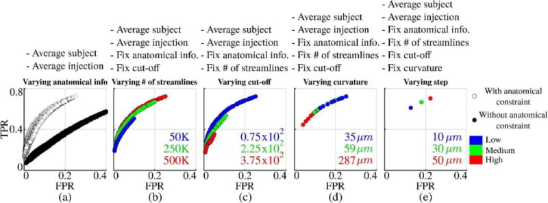
Summary of trends in tractography performance with respect to parameter changes. Data points show average values over all subjects and injection sites.

4.3. Results based on different tractography protocols are difficult to relate

Our study has significant conclusions owing to N-way ANOVA analysis. The variability in the overlap performance between subjects shown in Fig. 7 suggests that subject-wise comparisons should be done with caution. Our results show that performance variations introduced by different tractography parameter choices (for example cut-off) is comparable to variations introduced by different subjects. Additionally, our analysis indicate that all tractography parameters including step size and number of tracks significantly affect the performance. We found that varying injection locations and subjects affect overlap performance more than cut-off threshold, curvature and step size. Although a part of the associated differences might be due to registration errors or actual differences between subjects, we believe variation due to neuroanatomy and subjects is one of the major challenges in determining optimal parameters for tractography.

4.4. Improving tractography protocols and interpretation of results

Overall, our study points out to consider new practices for the application of tractography and how to interpret results:

• Our work reveals that neuroanatomy plays the most critical role in determining the performance of tractography, which underscores the importance of employing anatomical information in fiber tracking. This justifies the efforts to improve tractography via anatomical constraints (Smith et al. 2012) or atlases (Rojkova et al. 2016). However, even with perfect anatomical constraints, our results show that false negatives dominate the overlap performance which should be taken into account during the interpretation.

• The large variability in overlap quality due to injection locations shows that tractography techniques might provide better results if parameters are adjusted according to individual fiber bundles or regions of the brain that are being processed by the tracking algorithms.

• As a corollary to the previous points, we provide evidence that tractograms obtained for specific fiber bundles with optimized parameters and well-built anatomical constraints are more reliable compared to whole brain tractograms used for connectomics where there are limited opportunities for parameter optimization and anatomical restrictions. This makes tractography a more reliable tool to study certain parts of the brain than others.

• Our study heavily underlines the seriousness of documenting the complete list of tractography parameters. Because our N-way ANOVA analysis show that variations due to subjects and tractography parameters are comparable, the motivation to document the complete tractography protocol is beyond good practice. It is simply essential without which comparisons between different studies are potentially not meaningful.

• Our results showing the importance of all tractography parameters have implications in designing tractography protocols and how to decide parameters. Because results do converge with increasing number of tracks, it is good practice to study the convergence with respect to this parameter. On the other hand, our results show variability with respect to step size, curvature and cut-off parameters. Therefore conventional tractography studies that are based on a single set of parameter combination are prone to variations with respect to these parameters. One way to reduce biases due to fixed parameter choices is to repeat the experiments using different parameter combinations which would improve the reliability of results.

To conclude, we believe our findings will not only contribute to the literature of validation studies, but also improve our understanding on how to improve tractography experiments and interpret results.

References

- Aganj I, Lenglet C, Sapiro G, Yacoub E, Ugurbil K, Harel N. Reconstruction of the orientation distribution function in single-and multiple-shell q-ball imaging within constant solid angle. Magnetic Resonance in Medicine. 2010;64(2):554–566. doi: 10.1002/mrm.22365. [DOI] [PMC free article] [PubMed] [Google Scholar]
- Albi A, Meola A, Zhang F, Kahali P, Rigolo L, Tax CMW, Ciris PA, Essayed WI, Unadkat P, Norton I, Rathi Y, Olubiyi O, Golby AJ, O’Donnell LJ. Image Registration to Compensate for EPI Distortion in Patients with Brain Tumors: An Evaluation of Tract-Specific Effects. J Neuroimaging. 2018 doi: 10.1111/jon.12485. [DOI] [PMC free article] [PubMed] [Google Scholar]
- Avants BB, Tustison NJ, Song G, Cook PA, Klein A, Gee JC. A reproducible evaluation of ANTs similarity metric performance in brain image registration. Neuroimage. 2011;54(3):2033–2044. doi: 10.1016/j.neuroimage.2010.09.025. [DOI] [PMC free article] [PubMed] [Google Scholar]
- Aydogan DB, Shi Y. Probabilistic Tractography for Topographically Organized Connectomes. In: Ourselin S, Joskowicz L, Sabuncu MR, Unal G, Wells W, editors. Medical Image Computing and Computer-Assisted Intervention – MICCAI 2016. Springer International Publishing; Cham: 2016. pp. 201–209. (19th International Conference, Athens, Greece, October 17–21, 2016, Proceedings, Part I). [DOI] [PMC free article] [PubMed] [Google Scholar]
- Azadbakht H, Parkes LM, Haroon HA, Augath M, Logothetis NK, de Crespigny A, D’Arceuil HE, Parker GJ. Validation of High-Resolution Tractography Against In Vivo Tracing in the Macaque Visual Cortex. Cereb Cortex. 2015;25(11):4299–4309. doi: 10.1093/cercor/bhu326. [DOI] [PMC free article] [PubMed] [Google Scholar]
- Bach M, Fritzsche KH, Stieltjes B, Laun FB. Investigation of resolution effects using a specialized diffusion tensor phantom. Magnetic resonance in medicine. 2014;71(3):1108–1116. doi: 10.1002/mrm.24774. [DOI] [PubMed] [Google Scholar]
- Barazany D, Basser PJ, Assaf Y. In vivo measurement of axon diameter distribution in the corpus callosum of rat brain. Brain. 2009;132(Pt 5):1210–1220. doi: 10.1093/brain/awp042. [DOI] [PMC free article] [PubMed] [Google Scholar]
- Basser PJ, Mattiello J, LeBihan D. MR diffusion tensor spectroscopy and imaging. Biophysical Journal. 1994;66(1):259–267. doi: 10.1016/s0006-3495(94)80775-1. [DOI] [PMC free article] [PubMed] [Google Scholar]
- Basser PJ, Pajevic S, Pierpaoli C, Duda J, Aldroubi A. In vivo fiber tractography using DT-MRI data. Magn Reson Med. 2000;44(4):625–632. doi: 10.1002/1522-2594(200010)44:4<625::aid-mrm17>3.0.co;2-o. [DOI] [PubMed] [Google Scholar]
- Benson NC, Butt OH, Datta R, Radoeva PD, Brainard DH, Aguirre GK. The retinotopic organization of striate cortex is well predicted by surface topology. Curr Biol. 2012;22(21):2081–2085. doi: 10.1016/j.cub.2012.09.014. [DOI] [PMC free article] [PubMed] [Google Scholar]
- Besseling RM, Jansen JF, Overvliet GM, Vaessen MJ, Braakman HM, Hofman PA, Aldenkamp AP, Backes WH. Tract specific reproducibility of tractography based morphology and diffusion metrics. PloS one. 2012;7(4):e34125. doi: 10.1371/journal.pone.0034125. [DOI] [PMC free article] [PubMed] [Google Scholar]
- Budde MD, Janes L, Gold E, Turtzo LC, Frank JA. The contribution of gliosis to diffusion tensor anisotropy and tractography following traumatic brain injury: validation in the rat using Fourier analysis of stained tissue sections. Brain. 2011;134(Pt 8):2248–2260. doi: 10.1093/brain/awr161. [DOI] [PMC free article] [PubMed] [Google Scholar]
- Calabrese E, Badea A, Cofer G, Qi Y, Johnson GA. A diffusion MRI tractography connectome of the mouse brain and comparison with neuronal tracer data. Cerebral Cortex. 2015:bhv121. doi: 10.1093/cercor/bhv121. [DOI] [PMC free article] [PubMed] [Google Scholar]
- Calamante F, Tournier J-D, Kurniawan ND, Yang Z, Gyengesi E, Galloway GJ, Reutens DC, Connelly A. Super-resolution track-density imaging studies of mouse brain: comparison to histology. Neuroimage. 2012;59(1):286–296. doi: 10.1016/j.neuroimage.2011.07.014. [DOI] [PubMed] [Google Scholar]
- Campbell JS, Savadjiev P, Siddiqi K, Pike GB. Validation and regularization in diffusion MRI tractography; 3rd IEEE International Symposium on Biomedical Imaging: Nano to Macro; 2006. IEEE; 2006. pp. 351–354. [Google Scholar]
- Caruyer E, Lenglet C, Sapiro G, Deriche R. Design of multishell sampling schemes with uniform coverage in diffusion MRI. Magn Reson Med. 2013;69(6):1534–1540. doi: 10.1002/mrm.24736. [DOI] [PMC free article] [PubMed] [Google Scholar]
- Chen H, Liu T, Zhao Y, Zhang T, Li Y, Li M, Zhang H, Kuang H, Guo L, Tsien JZ. Optimization of large-scale mouse brain connectome via joint evaluation of DTI and neuron tracing data. NeuroImage. 2015a;115:202–213. doi: 10.1016/j.neuroimage.2015.04.050. [DOI] [PMC free article] [PubMed] [Google Scholar]
- Chen H, Liu T, Zhao Y, Zhang T, Li Y, Li M, Zhang H, Kuang H, Guo L, Tsien JZ, Liu T. Optimization of large-scale mouse brain connectome via joint evaluation of DTI and neuron tracing data. NeuroImage. 2015b;115:202–213. doi: 10.1016/j.neuroimage.2015.04.050. [DOI] [PMC free article] [PubMed] [Google Scholar]
- Chen H, Liu T, Zhao Y, Zhang T, Li Y, Li M, Zhang H, Kuang H, Guo L, Tsien JZ, Liu T. Optimization of large-scale mouse brain connectome via joint evaluation of DTI and neuron tracing data. Neuroimage. 2015c;115:202–213. doi: 10.1016/j.neuroimage.2015.04.050. [DOI] [PMC free article] [PubMed] [Google Scholar]
- Cheng J, Deriche R, Jiang T, Shen D, Yap P-T. Non-Negative Spherical Deconvolution (NNSD) for estimation of fiber Orientation Distribution Function in single-/multi-shell diffusion MRI. NeuroImage. 2014;101:750–764. doi: 10.1016/j.neuroimage.2014.07.062. [DOI] [PMC free article] [PubMed] [Google Scholar]
- Cote MA, Girard G, Bore A, Garyfallidis E, Houde JC, Descoteaux M. Tractometer: towards validation of tractography pipelines. Med Image Anal. 2013;17(7):844–857. doi: 10.1016/j.media.2013.03.009. [DOI] [PubMed] [Google Scholar]
- Daducci A, Dal Palù A, Lemkaddem A, Thiran J-P. COMMIT: convex optimization modeling for microstructure informed tractography. IEEE transactions on medical imaging. 2015;34(1):246–257. doi: 10.1109/TMI.2014.2352414. [DOI] [PubMed] [Google Scholar]
- Daianu M, Jahanshad N, Villalon-Reina JE, Prasad G, Jacobs RE, Barnes S, Zlokovic BV, Montagne A, Thompson PM. 7T Multi-shell Hybrid Diffusion Imaging (HYDI) for Mapping Brain Connectivity in Mice. Proc SPIE Int Soc Opt Eng. 2015:9413. doi: 10.1117/12.2081491. [DOI] [PMC free article] [PubMed] [Google Scholar]
- Dauguet J, Peled S, Berezovskii V, Delzescaux T, Warfield SK, Born R, Westin C-F. Comparison of fiber tracts derived from in-vivo DTI tractography with 3D histological neural tract tracer reconstruction on a macaque brain. Neuroimage. 2007;37(2):530–538. doi: 10.1016/j.neuroimage.2007.04.067. [DOI] [PubMed] [Google Scholar]
- Dice LR. Measures of the Amount of Ecologic Association between Species. Ecology. 1945;26(3):297–302. doi: 10.2307/1932409. [DOI] [Google Scholar]
- Donahue CJ, Sotiropoulos SN, Jbabdi S, Hernandez-Fernandez M, Behrens TE, Dyrby TB, Coalson T, Kennedy H, Knoblauch K, Van Essen DC, Glasser MF. Using Diffusion Tractography to Predict Cortical Connection Strength and Distance: A Quantitative Comparison with Tracers in the Monkey. J Neurosci. 2016;36(25):6758–6770. doi: 10.1523/JNEUROSCI.0493-16.2016. [DOI] [PMC free article] [PubMed] [Google Scholar]
- Dong HW. Allen Reference Atlas: A Digital Color Brain Atlas of the C57BL/6J Male Mouse. Wiley; New York: 2007. [Google Scholar]
- Dyrby TB, Søgaard LV, Parker GJ, Alexander DC, Lind NM, Baaré WF, Hay-Schmidt A, Eriksen N, Pakkenberg B, Paulson OB. Validation of in vitro probabilistic tractography. Neuroimage. 2007;37(4):1267–1277. doi: 10.1016/j.neuroimage.2007.06.022. [DOI] [PubMed] [Google Scholar]
- Feinberg DA, Moeller S, Smith SM, Auerbach E, Ramanna S, Gunther M, Glasser MF, Miller KL, Ugurbil K, Yacoub E. Multiplexed echo planar imaging for sub-second whole brain FMRI and fast diffusion imaging. PLoS One. 2010;5(12):e15710. doi: 10.1371/journal.pone.0015710. [DOI] [PMC free article] [PubMed] [Google Scholar]
- Ferizi U, Schneider T, Panagiotaki E, Nedjati-Gilani G, Zhang H, Wheeler-Kingshott CA, Alexander DC. A ranking of diffusion MRI compartment models with in vivo human brain data. Magn Reson Med. 2014;72(6):1785–1792. doi: 10.1002/mrm.25080. [DOI] [PMC free article] [PubMed] [Google Scholar]
- Fieremans E, De Deene Y, Delputte S, Özdemir MS, Achten E, Lemahieu I. The design of anisotropic diffusion phantoms for the validation of diffusion weighted magnetic resonance imaging. Physics in medicine and biology. 2008;53(19):5405. doi: 10.1088/0031-9155/53/19/009. [DOI] [PubMed] [Google Scholar]
- Fillard P, Descoteaux M, Goh A, Gouttard S, Jeurissen B, Malcolm J, Ramirez-Manzanares A, Reisert M, Sakaie K, Tensaouti F. Quantitative evaluation of 10 tractography algorithms on a realistic diffusion MR phantom. Neuroimage. 2011;56(1):220–234. doi: 10.1016/j.neuroimage.2011.01.032. [DOI] [PubMed] [Google Scholar]
- Girard G, Whittingstall K, Deriche R, Descoteaux M. Towards quantitative connectivity analysis: reducing tractography biases. Neuroimage. 2014;98:266–278. doi: 10.1016/j.neuroimage.2014.04.074. [DOI] [PubMed] [Google Scholar]
- Gyengesi E, Calabrese E, Sherrier MC, Johnson GA, Paxinos G, Watson C. Semi-automated 3D segmentation of major tracts in the rat brain: comparing DTI with standard histological methods. Brain Structure and Function. 2014;219(2):539–550. doi: 10.1007/s00429-013-0516-8. [DOI] [PMC free article] [PubMed] [Google Scholar]
- Heiervang E, Behrens T, Mackay C, Robson M, Johansen-Berg H. Between session reproducibility and between subject variability of diffusion MR and tractography measures. Neuroimage. 2006;33(3):867–877. doi: 10.1016/j.neuroimage.2006.07.037. [DOI] [PubMed] [Google Scholar]
- Heilingoetter CL, Jensen MB. Histological methods for ex vivo axon tracing: A systematic review. Neurol Res. 2016;38(7):561–569. doi: 10.1080/01616412.2016.1153820. [DOI] [PMC free article] [PubMed] [Google Scholar]
- Jbabdi S, Johansen-Berg H. Tractography: where do we go from here? Brain Connect. 2011;1(3):169–183. doi: 10.1089/brain.2011.0033. [DOI] [PMC free article] [PubMed] [Google Scholar]
- Jbabdi S, Lehman JF, Haber SN, Behrens TE. Human and monkey ventral prefrontal fibers use the same organizational principles to reach their targets: tracing versus tractography. The Journal of Neuroscience. 2013;33(7):3190–3201. doi: 10.1523/JNEUROSCI.2457-12.2013. [DOI] [PMC free article] [PubMed] [Google Scholar]
- Jbabdi S, Sotiropoulos SN, Haber SN, Van Essen DC, Behrens TE. Measuring macroscopic brain connections in vivo. Nat Neurosci. 2015;18(11):1546–1555. doi: 10.1038/nn.4134. [DOI] [PubMed] [Google Scholar]
- Jbabdi S, Sotiropoulos SN, Savio AM, Grana M, Behrens TE. Model-based analysis of multishell diffusion MR data for tractography: how to get over fitting problems. Magn Reson Med. 2012;68(6):1846–1855. doi: 10.1002/mrm.24204. [DOI] [PMC free article] [PubMed] [Google Scholar]
- Jenkinson M, Beckmann CF, Behrens TE, Woolrich MW, Smith SM. Fsl. Neuroimage. 2012;62(2):782–790. doi: 10.1016/j.neuroimage.2011.09.015. [DOI] [PubMed] [Google Scholar]
- Jeurissen B, Tournier J-D, Dhollander T, Connelly A, Sijbers J. Multi-tissue constrained spherical deconvolution for improved analysis of multi-shell diffusion MRI data. NeuroImage. 2014;103:411–426. doi: 10.1016/j.neuroimage.2014.07.061. [DOI] [PubMed] [Google Scholar]
- Kammen A, Law M, Tjan BS, Toga AW, Shi Y. Automated retinofugal visual pathway reconstruction with multi-shell HARDI and FOD-based analysis. Neuroimage. 2016;125:767–779. doi: 10.1016/j.neuroimage.2015.11.005. [DOI] [PMC free article] [PubMed] [Google Scholar]
- Keifer OP, Gutman DA, Hecht EE, Keilholz SD, Ressler KJ. A comparative analysis of mouse and human medial geniculate nucleus connectivity: a DTI and anterograde tracing study. NeuroImage. 2015;105:53–66. doi: 10.1016/j.neuroimage.2014.10.047. [DOI] [PMC free article] [PubMed] [Google Scholar]
- Knösche TR, Anwander A, Liptrot M, Dyrby TB. Validation of tractography: comparison with manganese tracing. Human brain mapping. 2015;36(10):4116–4134. doi: 10.1002/hbm.22902. [DOI] [PMC free article] [PubMed] [Google Scholar]
- Kuan L, Li Y, Lau C, Feng D, Bernard A, Sunkin SM, Zeng H, Dang C, Hawrylycz M, Ng L. Neuroinformatics of the allen mouse brain connectivity atlas. Methods. 2015;73:4–17. doi: 10.1016/j.ymeth.2014.12.013. [DOI] [PubMed] [Google Scholar]
- Leemans A, Sijbers J, Verhoye M, Van der Linden A, Van Dyck D. Mathematical framework for simulating diffusion tensor MR neural fiber bundles. Magnetic resonance in medicine. 2005;53(4):944–953. doi: 10.1002/mrm.20418. [DOI] [PubMed] [Google Scholar]
- Maier-Hein K, Neher P, Houde J-C, Cote M-A, Garyfallidis E, Zhong J, Chamberland M, Yeh F-C, Lin YC, Ji Q, Reddick WE, Glass JO, Chen DQ, Feng Y, Gao C, Wu Y, Ma J, Renjie H, Li Q, Westin C-F, Deslauriers-Gauthier S, Gonzalez JOO, Paquette M, St-Jean S, Girard G, Rheault F, Sidhu J, Tax CMW, Guo F, Mesri HY, David S, Froeling M, Heemskerk AM, Leemans A, Bore A, Pinsard B, Bedetti C, Desrosiers M, Brambati S, Doyon J, Sarica A, Vasta R, Cerasa A, Quattrone A, Yeatman J, Khan AR, Hodges W, Alexander S, Romascano D, Barakovic M, Auria A, Esteban O, Lemkaddem A, Thiran J-P, Cetingul HE, Odry BL, Mailhe B, Nadar M, Pizzagalli F, Prasad G, Villalon-Reina J, Galvis J, Thompson P, Requejo F, Laguna P, Lacerda L, Barrett R, Dell’Acqua F, Catani M, Petit L, Caruyer E, Daducci A, Dyrby T, Holland-Letz T, Hilgetag C, Stieltjes B, Descoteaux M. Tractography-based connectomes are dominated by false-positive connections. bioRxiv. 2016 doi: 10.1101/084137. [DOI] [Google Scholar]
- Mangin J-F, Fillard P, Cointepas Y, Le Bihan D, Frouin V, Poupon C. Toward global tractography. NeuroImage. 2013;80:290–296. doi: 10.1016/j.neuroimage.2013.04.009. [DOI] [PubMed] [Google Scholar]
- MathWorks I. MATLAB and Statistics Toolbox Release 2012. Natick: The MathWorks. Inc; 2012. [Google Scholar]
- Moeller S, Yacoub E, Olman CA, Auerbach E, Strupp J, Harel N, Ugurbil K. Multiband multislice GE-EPI at 7 tesla, with 16-fold acceleration using partial parallel imaging with application to high spatial and temporal whole-brain fMRI. Magn Reson Med. 2010;63(5):1144–1153. doi: 10.1002/mrm.22361. [DOI] [PMC free article] [PubMed] [Google Scholar]
- Mollink J, Kleinnijenhuis M, Cappellen van Walsum AV, Sotiropoulos SN, Cottaar M, Mirfin C, Heinrich MP, Jenkinson M, Pallebage-Gamarallage M, Ansorge O, Jbabdi S, Miller KL. Evaluating fibre orientation dispersion in white matter: Comparison of diffusion MRI, histology and polarized light imaging. Neuroimage. 2017;157:561–574. doi: 10.1016/j.neuroimage.2017.06.001. [DOI] [PMC free article] [PubMed] [Google Scholar]
- Mori S, Crain BJ, Chacko VP, van Zijl PC. Three-dimensional tracking of axonal projections in the brain by magnetic resonance imaging. Ann Neurol. 1999;45(2):265–269. doi: 10.1002/1531-8249(199902)45:2<265::aid-ana21>3.0.co;2-3. [DOI] [PubMed] [Google Scholar]
- Mukherjee P, Berman JI, Chung SW, Hess CP, Henry RG. Diffusion tensor MR imaging and fiber tractography: theoretic underpinnings. AJNR Am J Neuroradiol. 2008;29(4):632–641. doi: 10.3174/ajnr.A1051. [DOI] [PMC free article] [PubMed] [Google Scholar]
- Neher PF, Descoteaux M, Houde JC, Stieltjes B, Maier-Hein KH. Strengths and weaknesses of state of the art fiber tractography pipelines–A comprehensive in-vivo and phantom evaluation study using Tractometer. Med Image Anal. 2015;26(1):287–305. doi: 10.1016/j.media.2015.10.011. [DOI] [PubMed] [Google Scholar]
- Neher PF, Laun FB, Stieltjes B, Maier-Hein KH. Fiberfox: facilitating the creation of realistic white matter software phantoms. Magnetic resonance in medicine. 2014;72(5):1460–1470. doi: 10.1002/mrm.25045. [DOI] [PubMed] [Google Scholar]
- Nolte J. The human brain : an introduction to its functional anatomy. 6th. Mosby/Elsevier; Philadelphia, PA: 2009. [Google Scholar]
- Novikov DS, Jespersen SN, Kiselev VG, Fieremans E. Quantifying brain microstructure with diffusion MRI: Theory and parameter estimation. ArXiv e-prints. 2016:1612. doi: 10.1002/nbm.3998. [DOI] [PMC free article] [PubMed] [Google Scholar]
- Nucifora PG, Verma R, Lee SK, Melhem ER. Diffusion-tensor MR imaging and tractography: exploring brain microstructure and connectivity. Radiology. 2007;245(2):367–384. doi: 10.1148/radiol.2452060445. [DOI] [PubMed] [Google Scholar]
- Oh SW, Harris JA, Ng L, Winslow B, Cain N, Mihalas S, Wang Q, Lau C, Kuan L, Henry AM, Mortrud MT, Ouellette B, Nguyen TN, Sorensen SA, Slaughterbeck CR, Wakeman W, Li Y, Feng D, Ho A, Nicholas E, Hirokawa KE, Bohn P, Joines KM, Peng H, Hawrylycz MJ, Phillips JW, Hohmann JG, Wohnoutka P, Gerfen CR, Koch C, Bernard A, Dang C, Jones AR, Zeng H. A mesoscale connectome of the mouse brain. Nature. 2014;508(7495):207–214. doi: 10.1038/nature13186. [DOI] [PMC free article] [PubMed] [Google Scholar]
- Panagiotaki E, Schneider T, Siow B, Hall MG, Lythgoe MF, Alexander DC. Compartment models of the diffusion MR signal in brain white matter: A taxonomy and comparison. NeuroImage. 2012;59(3):2241–2254. doi: 10.1016/j.neuroimage.2011.09.081. [DOI] [PubMed] [Google Scholar]
- Partadiredja G, Miller R, Oorschot DE. The number, size, and type of axons in rat subcortical white matter on left and right sides: a stereological, ultrastructural study. J Neurocytol. 2003;32(9):1165–1179. doi: 10.1023/B:NEUR.0000021910.65920.41. [DOI] [PubMed] [Google Scholar]
- Pestilli F, Yeatman JD, Rokem A, Kay KN, Wandell BA. Evaluation and statistical inference for human connectomes. Nature methods. 2014;11(10):1058–1063. doi: 10.1038/nmeth.3098. [DOI] [PMC free article] [PubMed] [Google Scholar]
- Pullens P, Roebroeck A, Goebel R. Ground truth hardware phantoms for validation of diffusion- weighted MRI applications. Journal of Magnetic Resonance Imaging. 2010;32(2):482–488. doi: 10.1002/jmri.22243. [DOI] [PubMed] [Google Scholar]
- Reisert M, Kiselev VG, Dihtal B, Kellner E, Novikov DS. MesoFT: unifying diffusion modelling and fiber tracking. Med Image Comput Comput Assist Interv. 2014;17(Pt 3):201–208. doi: 10.1007/978-3-319-10443-0_26. [DOI] [PMC free article] [PubMed] [Google Scholar]
- Rojkova K, Volle E, Urbanski M, Humbert F, Dell’Acqua F, de Schotten MT. Atlasing the frontal lobe connections and their variability due to age and education: a spherical deconvolution tractography study. Brain Structure and Function. 2016;221(3):1751–1766. doi: 10.1007/s00429-015-1001-3. [DOI] [PubMed] [Google Scholar]
- Schmahmann JD, Pandya DN, Wang R, Dai G, D’Arceuil HE, de Crespigny AJ, Wedeen VJ. Association fibre pathways of the brain: parallel observations from diffusion spectrum imaging and autoradiography. Brain. 2007;130(3):630–653. doi: 10.1093/brain/awl359. [DOI] [PubMed] [Google Scholar]
- Seehaus AK, Roebroeck A, Chiry O, Kim D-S, Ronen I, Bratzke H, Goebel R, Galuske RA. Histological validation of DW-MRI tractography in human postmortem tissue. Cerebral cortex. 2012:bhs036. doi: 10.1093/cercor/bhs036. [DOI] [PMC free article] [PubMed] [Google Scholar]
- Sergejeva M, Papp EA, Bakker R, Gaudnek MA, Okamura-Oho Y, Boline J, Bjaalie JG, Hess A. Anatomical landmarks for registration of experimental image data to volumetric rodent brain atlasing templates. J Neurosci Methods. 2015;240:161–169. doi: 10.1016/j.jneumeth.2014.11.005. [DOI] [PubMed] [Google Scholar]
- Setsompop K, Gagoski BA, Polimeni JR, Witzel T, Wedeen VJ, Wald LL. Blipped-controlled aliasing in parallel imaging for simultaneous multislice echo planar imaging with reduced g-factor penalty. Magn Reson Med. 2012;67(5):1210–1224. doi: 10.1002/mrm.23097. [DOI] [PMC free article] [PubMed] [Google Scholar]
- Shattuck DW, Leahy RM. BrainSuite: an automated cortical surface identification tool. Medical image analysis. 2002;6(2):129–142. doi: 10.1016/s1361-8415(02)00054-3. [DOI] [PubMed] [Google Scholar]
- Smith RE, Tournier J-D, Calamante F, Connelly A. Anatomically-constrained tractography: improved diffusion MRI streamlines tractography through effective use of anatomical information. Neuroimage. 2012;62(3):1924–1938. doi: 10.1016/j.neuroimage.2012.06.005. [DOI] [PubMed] [Google Scholar]
- Smith RE, Tournier J-D, Calamante F, Connelly A. SIFT2: Enabling dense quantitative assessment of brain white matter connectivity using streamlines tractography. Neuroimage. 2015;119:338–351. doi: 10.1016/j.neuroimage.2015.06.092. [DOI] [PubMed] [Google Scholar]
- Sotiropoulos SN, Hernandez-Fernandez M, Vu AT, Andersson JL, Moeller S, Yacoub E, Lenglet C, Ugurbil K, Behrens TEJ, Jbabdi S. Fusion in diffusion MRI for improved fibre orientation estimation: An application to the 3T and 7T data of the Human Connectome Project. Neuroimage. 2016;134:396–409. doi: 10.1016/j.neuroimage.2016.04.014. [DOI] [PMC free article] [PubMed] [Google Scholar]
- Thomas C, Frank QY, Irfanoglu MO, Modi P, Saleem KS, Leopold DA, Pierpaoli C. Anatomical accuracy of brain connections derived from diffusion MRI tractography is inherently limited. Proceedings of the National Academy of Sciences. 2014;111(46):16574–16579. doi: 10.1073/pnas.1405672111. [DOI] [PMC free article] [PubMed] [Google Scholar]
- Toga AW, Clark KA, Thompson PM, Shattuck DW, Van Horn JD. Mapping the Human Connectome. Neurosurgery. 2012;71(1):1–5. doi: 10.1227/neu.0b013e318258e9ff. [DOI] [PMC free article] [PubMed] [Google Scholar]
- Tournier J-D, Calamante F, Gadian DG, Connelly A. Direct estimation of the fiber orientation density function from diffusion-weighted MRI data using spherical deconvolution. NeuroImage. 2004;23(3):1176–1185. doi: 10.1016/j.neuroimage.2004.07.037. [DOI] [PubMed] [Google Scholar]
- Tournier J, Calamante F, Connelly A. Improved probabilistic streamlines tractography by 2nd order integration over fibre orientation distributions. Proc 18th Annual Meeting of the Intl Soc Mag Reson Med(ISMRM) 2010:1670. [Google Scholar]
- Tournier JD, Calamante F, Connelly A. MRtrix: Diffusion tractography in crossing fiber regions. Int J Imaging Syst Technol. 2012;22(1):53–66. doi: 10.1002/ima.22005. [DOI] [Google Scholar]
- Tran G, Shi Y. Fiber orientation and compartment parameter estimation from multi-shell diffusion imaging. IEEE transactions on medical imaging. 2015;34(11):2320–2332. doi: 10.1109/TMI.2015.2430850. [DOI] [PMC free article] [PubMed] [Google Scholar]
- Tuch DS. Q-ball imaging. Magnetic resonance in medicine. 2004;52(6):1358–1372. doi: 10.1002/mrm.20279. [DOI] [PubMed] [Google Scholar]
- Tuch DS, Reese TG, Wiegell MR, Makris N, Belliveau JW, Wedeen VJ. High angular resolution diffusion imaging reveals intravoxel white matter fiber heterogeneity. Magn Reson Med. 2002;48(4):577–582. doi: 10.1002/mrm.10268. [DOI] [PubMed] [Google Scholar]
- Van Essen DC, Smith SM, Barch DM, Behrens TE, Yacoub E, Ugurbil K, Consortium WU-MH The WU-Minn Human Connectome Project: an overview. Neuroimage. 2013;80:62–79. doi: 10.1016/j.neuroimage.2013.05.041. [DOI] [PMC free article] [PubMed] [Google Scholar]
- Wandell BA. Clarifying Human White Matter. Annu Rev Neurosci. 2016;39:103–128. doi: 10.1146/annurev-neuro-070815-013815. [DOI] [PubMed] [Google Scholar]
- Wedeen VJ, Hagmann P, Tseng WYI, Reese TG, Weisskoff RM. Mapping complex tissue architecture with diffusion spectrum magnetic resonance imaging. Magnetic resonance in medicine. 2005;54(6):1377–1386. doi: 10.1002/mrm.20642. [DOI] [PubMed] [Google Scholar]
- Willats L, Raffelt D, Smith RE, Tournier JD, Connelly A, Calamante F. Quantification of track-weighted imaging (TWI): characterisation of within-subject reproducibility and between-subject variability. Neuroimage. 2014;87:18–31. doi: 10.1016/j.neuroimage.2013.11.016. [DOI] [PubMed] [Google Scholar]
- Wu D, Martin LJ, Northington FJ, Zhang J. Oscillating gradient diffusion MRI reveals unique microstructural information in normal and hypoxia-ischemia injured mouse brains. Magn Reson Med. 2014;72(5):1366–1374. doi: 10.1002/mrm.25441. [DOI] [PMC free article] [PubMed] [Google Scholar]
- Wu D, Xu J, McMahon MT, van Zijl PC, Mori S, Northington FJ, Zhang J. In vivo high-resolution diffusion tensor imaging of the mouse brain. Neuroimage. 2013;83:18–26. doi: 10.1016/j.neuroimage.2013.06.012. [DOI] [PMC free article] [PubMed] [Google Scholar]
- Yamada K, Sakai K, Akazawa K, Yuen S, Nishimura T. MR tractography: a review of its clinical applications. Magn Reson Med Sci. 2009;8(4):165–174. doi: 10.2463/mrms.8.165. [DOI] [PubMed] [Google Scholar]
- Yeh CH, Smith RE, Liang X, Calamante F, Connelly A. Correction for diffusion MRI fibre tracking biases: The consequences for structural connectomic metrics. Neuroimage. 2016 doi: 10.1016/j.neuroimage.2016.05.047. [DOI] [PubMed] [Google Scholar]
- Yeh FC, Wedeen VJ, Tseng WY. Generalized q-sampling imaging. IEEE Trans Med Imaging. 2010;29(9):1626–1635. doi: 10.1109/TMI.2010.2045126. [DOI] [PubMed] [Google Scholar]
- Zingg B, Hintiryan H, Gou L, Song MY, Bay M, Bienkowski MS, Foster NN, Yamashita S, Bowman I, Toga AW, Dong HW. Neural networks of the mouse neocortex. Cell. 2014;156(5):1096–1111. doi: 10.1016/j.cell.2014.02.023. [DOI] [PMC free article] [PubMed] [Google Scholar]
Associated Data
This section collects any data citations, data availability statements, or supplementary materials included in this article.