Blind deconvolution estimation of fluorescence measurements through quadratic programming

Abstract.

Time-deconvolution of the instrument response from fluorescence lifetime imaging microscopy (FLIM) data is usually necessary for accurate fluorescence lifetime estimation. In many applications, however, the instrument response is not available. In such cases, a blind deconvolution approach is required. An iterative methodology is proposed to address the blind deconvolution problem departing from a dataset of FLIM measurements. A linear combination of a base conformed by Laguerre functions models the fluorescence impulse response of the sample at each spatial point in our formulation. Our blind deconvolution estimation (BDE) algorithm is formulated as a quadratic approximation problem, where the decision variables are the samples of the instrument response and the scaling coefficients of the basis functions. In the approximation cost function, there is a bilinear dependence on the decision variables. Hence, due to the nonlinear nature of the estimation process, an alternating least-squares scheme iteratively solves the approximation problem. Our proposal searches for the samples of the instrument response with a global perspective, and the scaling coefficients of the basis functions locally at each spatial point. First, the iterative methodology relies on a least-squares solution for the instrument response, and quadratic programming for the scaling coefficients applied just to a subset of the measured fluorescence decays to initially estimate the instrument response to speed up the convergence. After convergence, the final stage computes the fluorescence impulse response at all spatial points. A comprehensive validation stage considers synthetic and experimental FLIM datasets of ex vivo atherosclerotic plaques and human breast cancer cell samples that highlight the advantages of the proposed BDE algorithm under different noise and initial conditions in the iterative scheme and parameters of the proposal.

1. Introduction

Fluorescence microscopy imaging is a powerful noninvasive technique that allows a biochemical characterization of biological tissue for medical and biophysical applications.^1–4 Specifically, multispectral fluorescence lifetime imaging microscopy (m-FLIM) captures the time-resolved response to a laser excitation at different spectral channels in order to record the optical emission of synthetic or endogenous fluorophores.⁵ Different studies in the literature have shown the potential of FLIM information for providing an early and noninvasive diagnosis tool for different pathologies, as cardiovascular and dermatology diseases,^6–9 oral precancer conditions,¹⁰ colonic dysplasia,¹¹ or measuring therapeutic responses of anticancer drugs.^12,13 In order to provide quantitative evaluations of m-FLIM information, the datasets are first processed to isolate the instrument signature and extract the intrinsic fluorescence response of the studied sample. Departing from a linear interaction in the measured fluorescence decay due to the optic excitation, a convolution model is adopted where the fluorescence impulse response denotes the distinctive signature of the sample that is usually characterized by a multiexponential model^14–16 or by a Laguerre basis.^17–19 This process is usually called deconvolution in the FLIM literature.^1–4 Once the fluorescence impulse response has been identified at each spatial point of the sample, the lifetime per spectral channel and normalized intensities are used to provide quantitative features for classification purposes of the m-FLIM dataset.¹⁰ Meanwhile, a graphical perspective is the phasor approach that provides a two-dimensional (2-D) visual representation of each spatial point in the dataset by mapping the identified fluorescence impulse response per spectral band. Classification or linear unmixing can be achieved from this 2-D representation, as suggested in Ref. 20 and 21.

The main two trends in deconvolution algorithms depend on the structure of the fluorescence impulse response. The first approach assumes a linear combination of exponential functions that characterize the response of each fluorophore in the sample.^4,13 Thus, the free parameters in this model are the characteristic times for the exponential functions and their scaling coefficients. In this case, the scalings are linear variables in the model, but the characteristic times exhibit a nonlinear dependency. Hence, a nonlinear approximation problem is formulated to compute the free variables and minimize the prediction error, which can be iteratively solved by nonlinear least squares^22,23 for each spatial point in the sample. Furthermore, if the characteristic times are assumed invariant in all the samples, then there are few parameters involved in the optimization scheme, and this concept is called the global approach.^14–16 Meanwhile, in Refs. ²⁴ and ²⁵, by addressing the properties of the optical instrumentation, the exponential profiles can be affected by uncertainty in the photon counts, which can be modeled as Poisson noise. Thus, the problem of Poisson–Gaussian parameter estimation has recently caught the attention of the scientific community. On the other hand, the second approach for deconvolution considers that a linear combination of discrete-time Laguerre functions models the fluorescence impulse response; this technique is referred to as the model-free scheme. In this way, the scaling coefficients of the Laguerre functions are linear variables in the residual, so a least-squares estimation can be followed.^17,18 One disadvantage of the Laguerre basis is that for some cases, the resulting fluorescence impulse responses might not have a monotonic decay. Therefore, a constrained quadratic optimization has to be applied to compute the scaling coefficients, where the restrictions are imposed to the second- or third-order time derivatives of the resulting fluorescence impulse responses.¹⁹

One disadvantage of the deconvolution algorithms from the literature is the requirement of a previous recording of the FLIM instrument response. In addition, while computing the deconvolution methodology, the instrument response has to be carefully aligned with the fluorescence decay measurements in order to avoid dead-times, which could be a time-consuming task due to noise, and could also bias the lifetime estimations. Hence, the contribution of this work is to present a blind deconvolution estimation (BDE) algorithm that does not require previous knowledge of the instrument response in the m-FLIM setup. For this purpose, we consider that the fluorescence impulse response is characterized by a linear combination of Laguerre functions. Our BDE algorithm searches for the instrument response samples with a global perspective, meanwhile the scaling coefficients of the basis functions are computed for each point in the sample. Since the residual exhibits a bilinear dependency on the decision variables, and alternating least-squares (ALS) methodology iteratively estimates the instrument response and scaling variables.^26,27 The recurrent steps in the BDE algorithm rely on constrained quadratic programming and least-squares solutions. In this way, our BDE method jointly provides an estimation of the instrument and fluorescence impulse responses in the sample. Our synthetic and experimental results with ex vivo atherosclerotic plaques and human breast cancer cell samples show that the proposal is robust to uncertainty in the measured fluorescence decays and variations in the initial conditions.

The notation used in this paper is described next. Scalars are denoted by italic letters, and vectors and matrices by lower-case and upper-case bold letters, respectively. $\mathbb{R}$ and $\mathbb{Z}$ represent the real and integer numbers, ${\mathbb{R}}^N$ $N$-dimensional real vectors, and $\mathrm{card}(\mathrm{\Omega })$ the cardinality of a set $\mathrm{\Omega }$. For a real vector $\mathbf{x}$, the transpose operation is denoted by ${\mathbf{x}}^{\top }$, the Euclidean norm by ${\Vert \mathbf{x}\Vert }_2=\sqrt{{\mathbf{x}}^{\top }\mathbf{x}}$, and $\mathbf{x}⪰0$ represents that each component in the vector is positive or zero. For a square matrix $\mathbf{X}\in {\mathbb{R}}^{N\times N}$, $X_{i,j}$ represents the element in the $i$’th row and $j$’th column ($i,j\in [1,N]$), $\mathrm{Tr}(\mathbf{X})=\sum _i{X}_{i,i}$ denotes the trace operation, ${\Vert \mathbf{X}\Vert }_F=\sqrt{\mathrm{Tr}({\mathbf{X}}^{\top }\mathbf{X})}$ denotes the Frobenius norm, and ${\Vert \mathbf{X}\Vert }_{\infty }={\max }_i\sum _{j=1}^N|X_{i,j}|$ denotes the maximum absolute row sum norm. $\mathbf{X}⪰0$ represents that each component in the matrix is non-negative. ${\mathbf{Y}}_{a:b}\in {\mathbb{R}}^{(b-a+1)\times M}$ represents the block matrix extracted from $\mathbf{Y}\in {\mathbb{R}}^{N\times M}$ by its rows $a$ to $b$ ($1\le a<b\le N$). For all vectors $\mathbf{x}\in {\mathbb{R}}^N$ and $\mathbf{y}\in {\mathbb{R}}^M$, $T_{\mathbf{x},\mathbf{y}}\in {\mathbb{R}}^{N\times M}$ denotes a toeplitz matrix with $\mathbf{x}$ and ${\mathbf{y}}^{\top }$ as its first column and row, respectively, where the first entry in $\mathbf{x}$ and $\mathbf{y}$ must be equal. An $N$-dimensional vector filled with ones (zeros) is represented by ${\mathbf{1}}_N$ (${\mathbf{0}}_N$), and ${\mathbf{I}}_N$ denotes the identity matrix of order $N$. For a random variable $x$, $x\sim \mathcal{U}[a,b]$ represents that $x$ is uniformly distributed in the interval $[a,b]$ ($b>a$), and $x\sim \mathcal{N}(0,{\sigma }^2)$ that $x$ is normally distributed with zero mean and variance ${\sigma }^2$.

2. Problem Formulation

First, the deconvolution of FLIM data is expressed in discrete time by assuming that the measured fluorescence decays and instrument response are sampled with a period $T$ over a spatial domain of $K$ points in the dataset.^1–3 Therefore, by considering a time window of $L$ samples and a causal response,²⁸ the observation model for the $l$’th time sample and $k$’th spatial point is given by

$$y_k[l]=u[l]\star h_k[l]+v_k[l]$$ (1)

$$=\sum _{j=0}^{L-1}u[l-j]h_k[j]+v_k[l]\forall l\in [0,L-1],k\in [0,K-1],$$ (2)

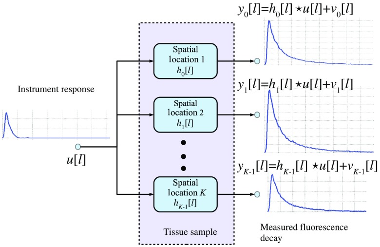
where $y_k[l]$, $u[l]$, and $h_k[l]$ denote the measured fluorescence decay, instrument response, and fluorescence impulse response samples, respectively, $\star$; stands for the convolution operation, and $v_k[l]$ represents the random noise related to the instrumentation or measurement uncertainty. A block diagram of the observation model in our formulation is presented in Fig. 1. In our framework, the effect of scattering can be modeled as a scaled factor $A_k>0$ of the instrument response in the observation model,^4,13 i.e., $y_k[l]=(h_k[l]+A_k\delta [l])\star u[l]+v_k[l]$, where $\delta [l]$ denotes the discrete-time delta function. Therefore, the estimation of the instrument response $u[l]$ will not be affected by the scattering component, since the structure of the observation model is not modified with respect to $u[l]$. Although this component could potentially introduce a distortion of the estimated impulse response function, that is, $(h_k[l]+A_k\delta [l])$ instead of $h_k[l]$, this a common problem to all deconvolution methods. However, it has been shown that the scattering effect is not significant for endogenous tissue FLIM.²⁹ In general, the deconvolution formulation is an ill-posed inverse problem that can have multiple solutions.^1–3 Therefore, to restrict the search space and to have a tractable problem, in our formulation, there are two key assumptions:

Fig. 1.

Fluorescence lifetime imaging microscopy (FLIM) observation model.

• 1.
  The instrument response $u[l]$ is common to all $K$ spatial points in the dataset, and its samples are non-negative and normalized to sum one in time domain, i.e.,

  $$\sum _{l=0}^{L-1}u[l]=1\text{and}u[l]\ge 0\forall l\in [0,L-1],$$ (3)
• 2.The fluorescence impulse response $h_k[l]$ at each spatial sample $k$ and time instant $l$ can be represented by a linear combination of $N$ discrete-time basis functions ${\{b_n[l]\}}_{n=0}^{N-1}$ also common to all the spatial points.

Assumption 1 allows to restrict the search among all possible instrument responses, and to avoid numerical scaling problems in the estimation of $u[l]$. Nonetheless, the shape of the resulting instrument response is not limited as our validation section will show. Meanwhile, assumption 2 allows to formulate the estimation problem as constrained quadratic programming or least-squares approximations, which can be efficiently solve by numerical optimization algorithms.²³ These two conditions will be exploited to achieve the blind deconvolution of the dataset as explained next. First, the observation model in Eq. (1) can be written in a vector notation as

$$\underset{{\mathbf{y}}_k\in {\mathbb{R}}^L}{\underbrace{\left[\begin{array}{c}{y}_k[0]\\ y_k[1]\\ ⋮\\ y_k[L-1]\end{array}\right]}}=\underset{\mathbf{U}\in {\mathbb{R}}^{L\times L}}{\underbrace{\left[\begin{array}{cccc}u[0]& 0& \dots & 0\\ u[1]& u[0]& \dots & 0\\ ⋮& ⋮& \ddots & ⋮\\ u[L-1]& u[L-2]& \dots & u[0]\end{array}\right]}}\underset{{\mathbf{h}}_k\in {\mathbb{R}}^L}{\underbrace{\left[\begin{array}{c}{h}_k[0]\\ h_k[1]\\ ⋮\\ h_k[L-1]\end{array}\right]}}+\underset{{\mathbf{v}}_k\in {\mathbb{R}}^L}{\underbrace{\left[\begin{array}{c}{v}_k[0]\\ v_k[1]\\ ⋮\\ v_k[L-1]\end{array}\right]}},$$ (4)

$$\Rightarrow {\mathbf{y}}_k=\mathbf{U}{\mathbf{h}}_k+{\mathbf{v}}_k\forall k\in [0,K-1],$$ (5)

and as a result, the input matrix $\mathbf{U}$ has a toeplitz structure³⁰ that does not depend on the spatial location of the sample. In this matrix formulation, the restrictions in Eq. (3) for the instrument response can be written as

$${\Vert \mathbf{U}\Vert }_{\infty }=1\text{and}\mathbf{U}⪰0$$ (6)

Next, by assumption 2, the fluorescence impulse response at $k$’th spatial location is characterized by the scaling coefficients ${\{c_{k,n}\}}_{n=0}^{N-1}$ of the basis functions:

$$h_k[l]=\sum _{n=0}^{N-1}{c}_{k,n}{b}_n[l]\forall l\in [0,L-1],$$ (7)

where the coefficients $c_{k,n}\in \mathbb{R}$ are selected such that the estimated fluorescence decay matches the measurement, and the resulting time-response has some smoothness property to represent the response of biological samples.^17–19 The fluorescence impulse responses estimated from FLIM data involve some smoothness properties that in turn constrain the linear model in Eq. (7).^1–3 Hence, the estimated response must be monotonically decreasing to have a biological meaning at any spatial point. As a result, the time derivative of the fluorescence impulse response has to be negative definite ($h_k^{\prime }<0$ $\forall k$), but without inflection points or curvature changes. Thus, an alternative restriction is to consider a positive definite condition on the second-order time derivative ($h_k^{\prime \prime }>0$), or a negative semidefinite on the third-order derivative ($h_k^{\prime \prime \prime }\le 0$).¹⁹ The instantaneous expression in Eq. (7) can be also written in vector notation to gather all the time samples as

$${\mathbf{h}}_k=\mathbf{B}{\mathbf{c}}_k\forall k\in [0,K-1],$$ (8)

where

$$\mathbf{B}=\left[\begin{array}{cccc}{b}_0[0]& b_1[0]& \dots & b_{N-1}[0]\\ b_0[1]& b_1[1]& \dots & b_{N-1}[1]\\ ⋮& ⋮& \ddots & ⋮\\ b_0[L-1]& b_1[L-1]& \dots & b_{N-1}[L-1]\end{array}\right]\in {\mathbb{R}}^{L\times N},$$ (9)

$${\mathbf{c}}_k={[c_{k,0}\dots c_{k,N-1}]}^{\top }\in {\mathbb{R}}^N.$$ (10)

In the analysis of FLIM measurements, a well-known basis is the Laguerre functions:^17–19

$$b_n[l]={\alpha }^{\frac{1}{2}(l-n)}\sqrt{1-\alpha }\sum _{i=0}^n{(-1)}^i(l_i)(n_i){\alpha }^{n-i}{(1-\alpha )}^i\forall n\in [0,N-1],l\in [0,L-1],$$ (11)

where $\alpha \in (0,1)$ is a free parameter. Consequently, by considering measurement noise, the observation model in Eq. (1) can be compactly expressed as

$${\mathbf{y}}_k={\mathbf{UBc}}_k+{\mathbf{v}}_k\forall k\in [0,K-1].$$ (12)

By collecting all the spatial measurements in a matrix notation, the following model is obtained

$$\mathbf{Y}=\mathbf{UBC}+\mathbf{V},$$ (13)

where

$$\mathbf{Y}=[{\mathbf{y}}_0\dots {\mathbf{y}}_{K-1}]\in {\mathbb{R}}^{L\times K},$$ (14)

$$\mathbf{C}=[{\mathbf{c}}_0\dots {\mathbf{c}}_{N-1}]\in {\mathbb{R}}^{N\times K},$$ (15)

$$\mathbf{V}=[{\mathbf{v}}_0\dots {\mathbf{v}}_{K-1}]\in {\mathbb{R}}^{L\times K}.$$ (16)

In this way, according to the observation model in Eq. (13), the blind deconvolution problem is jointly defined as obtaining the input and coefficients matrices $(\mathbf{U},\mathbf{C})$ to approximate the measurements information $\mathbf{Y}$. Hence, our methodology can be formulated as an optimal quadratic approximation problem:²³

$$\begin{gathered} \underset{\mathbf{U},\mathbf{C}}{\min }\underset{J}{\underbrace{\frac{1}{2}{\Vert \mathbf{Y}-\mathbf{UBC}\Vert }_F^2}}, \\ \text{such that\hspace{0.17em}\hspace{0.17em}}{\Vert \mathbf{U}\Vert }_{\infty }=1\text{and}\mathbf{U}⪰0. \end{gathered}$$ (17)

Therefore, there is a nonlinear interaction in the cost function $J$ between the optimization variables $\mathbf{U}$ and $\mathbf{C}$. One important advantage of the previous formulation is that the input matrix $\mathbf{U}$ has a toeplitz structure.³⁰ Therefore, to construct this matrix, only $L$ values are needed. Moreover, in FLIM applications, the instrument response is a narrow pulse, so there is no need to estimate all the $L$ terms, since many will be zero. Hence, we consider only the first $\widehat{L}$ terms $(\widehat{L}<L)$ to represent the instrument response. In this way, the input matrix $\mathbf{U}$ in Eq. (4) can be parametrized as a linear combination of $\widehat{L}$ toeplitz matrices ${\mathbf{U}}_l^o\in {\mathbb{R}}^{L\times L}$

$$\mathbf{U}=\sum _{l=0}^{\widehat{L}-1}{\theta }_l{\mathbf{U}}_l^o,$$ (18)

where the parameter ${\theta }_l=u[l]$ represents $l$’th sample in the instrument response, and

$${\mathbf{U}}_l^o={\mathbf{T}}_{{\mathbf{x}}_l,{\mathbf{y}}_l}\in {\mathbb{R}}^{L\times L},$$ (19)

$${\mathbf{x}}_l={[{\mathbf{0}}_l^{\mathrm{T}}1{\mathbf{0}}_{L-l-1}^{\mathrm{T}}]}^{\top }\in {\mathbb{R}}^L,$$ (20)

$${\mathbf{y}}_l={[1{\mathbf{0}}_{L-1}^{\mathrm{T}}]}^{\top }\in {\mathbb{R}}^L.$$ (21)

To illustrate the toeplitz structure of matrices ${\mathbf{U}}_l^o$, the corresponding ones for indices $l=0,1$ and 2 are shown next

$${\mathbf{U}}_0^o={\mathbf{I}}_L,{\mathbf{U}}_1^o=\left[\begin{array}{ccccc}0& 0& \dots & 0& 0\\ 1& 0& \dots & 0& 0\\ 0& 1& \dots & 0& 0\\ ⋮& ⋮& \ddots & ⋮& ⋮\\ 0& 0& \dots & 1& 0\end{array}\right],{\mathbf{U}}_2^o=\left[\begin{array}{cccccc}0& 0& \dots & 0& 0& 0\\ 0& 0& \dots & 0& 0& 0\\ 1& 0& \dots & 0& 0& 0\\ 0& 1& \dots & 0& 0& 0\\ ⋮& ⋮& \ddots & ⋮& ⋮& ⋮\\ 0& 0& \dots & 1& 0& 0\end{array}\right].$$ (22)

One advantage of the parametric representation in Eq. (18) is that the normalization condition in Eq. (3) for the instrument response can be easily incorporated into the optimization formulation. In this way, the blind deconvolution scheme in Eq. (17) can be rewritten as

$$\begin{gathered} \underset{{\{{\theta }_l\}}_{l=0}^{\widehat{L}-1},\mathbf{C}}{\min }\frac{1}{2}{\Vert \mathbf{Y}-\sum _{l=0}^{\widehat{L}-1}{\theta }_l{\mathbf{U}}_l^o\mathbf{BC}\Vert }_F^2 \\ \text{such that\hspace{0.17em}\hspace{0.17em}}\sum _l{\theta }_l=1\text{and}{\theta }_l\ge 0\forall l\in [0,\widehat{L}-1]. \end{gathered}$$ (23)

3. Time Restrictions on the Fluorescence Impulse Response

In Ref. 19, to facilitate the computation of the scaling coefficients through numerical optimization, a negative semidefinite condition ($h_k^{\prime \prime \prime }\le 0$) is imposed on the third-order time derivative (NSC-TOTD). This restriction can be written as a linear vector inequality for the scaling coefficients ${\mathbf{c}}_k$ in Eq. (8) at $k$’th spatial location. For this purpose, we employ a numerical approximation for the TOTD based on the central difference approach for $l$’th time instant and $k$’th spatial point:²²

$$h_k^{\prime \prime \prime }[l]=\frac{-h_k[l+3]+8h_k[l+2]-13h_k[l+1]+13h_k[l-1]-8h_k[l-2]+h_k[l-3]}{8T^3},$$ (24)

where to evaluate $h_k^{\prime \prime \prime }[l]$ besides the $l$’th sample, six more time samples are needed. Therefore, by using a vector notation, the discrete-time approximation of the TOTD of the fluorescence impulse response at $k$’th spatial location is

$${{\mathbf{h}}^{\prime \prime \prime }}_k=\mathbf{A}{\mathbf{c}}_k\in {\mathbb{R}}^{L-6},$$ (25)

where

$$\mathbf{A}\triangleq \frac{1}{8T^3}(-{\mathbf{B}}_{7:L}+8{\mathbf{B}}_{6:L-1}-13{\mathbf{B}}_{5:L-2}+13{\mathbf{B}}_{3:L-4}-8{\mathbf{B}}_{2:L-5}+{\mathbf{B}}_{1:L-6})\in {\mathbb{R}}^{(L-6)\times N}.$$ (26)

Following this vector notation, the following linear vector inequality can represent the time-domain restrictions on the fluorescence impulse response for the scaling coefficients ${\mathbf{c}}_k$ at the $k$’th spatial point:

$${\mathbf{Ac}}_k\le 0\forall k\in [0,K-1].$$ (27)

4. Quadratic Optimal Approximation

From the previous results in Eqs. (23) and (27), the blind deconvolution problem with time-domain restrictions in the fluorescence impulse response can be formulated as a quadratic constrained optimization scheme with linear equality and inequality conditions

$$\begin{gathered} \underset{{\{{\theta }_l\}}_{l=0}^{\widehat{L}-1},\mathbf{C}}{\min }\frac{1}{2}{\Vert \mathbf{Y}-\sum _{l=0}^{\widehat{L}-1}{\theta }_l{\mathbf{U}}_l^o\mathbf{BC}\Vert }_F^2 \\ \text{such that\hspace{0.17em}\hspace{0.17em}}\sum _l{\theta }_l=1,{\theta }_l\ge 0\forall l\in [0,\widehat{L}-1],{\mathbf{Ac}}_k\le \mathbf{b}\forall k\in [0,K-1]. \end{gathered}$$ (28)

The proposed optimization scheme in Eq. (28) has a particular structure that has not been investigated in the literature so far. For example, in linear unmixing problems or non-negative matrix factorization,^27,31–33 the measured fluorescence decays matrix $\mathbf{Y}$ is decomposed as the product of two matrices that have certain properties: positivity and/or normalization conditions. However, in Eq. (28), the parametric structure of the decision variables ${\theta }_l$ and the presence of the product matrix ${\mathbf{U}}_l^o\mathbf{B}$ oversee a new formulation. In fact, since the cost function in Eq. (28) involves the product of the decision variables ${\left(\right\{{\theta }_l\}}_{l=0}^{\widehat{L}-1},\mathbf{C})$, and the constraints can be divided into time-domain and spatial restrictions, similar to Refs. ²⁶, 27, and 31, a solution based on ALS is pursued. Hence, first given an initial condition for the unknown parameters

$${\mathit{\theta }}^0={[{\mathit{\theta }}_0^0,{\mathit{\theta }}_1^0,\dots ,{\mathit{\theta }}_{\widehat{L}-1}^0]}^{\top },$$

the optimal scaling coefficients ${\mathbf{c}}_k$ are calculated for each spatial location $k$ by an optimal approximation method. The initial instrument response vector ${\theta }^0$ can be chosen from some a priori information, or as a general square pulse. In this work, we also consider a signal that employs the mean spatial measurements of the FLIM dataset to shape the initial input vector. Next, fixing the coefficients ${\mathbf{c}}_k$ and considering the whole dataset, our proposal calculates the optimal instrument response sequence $\mathit{\theta }={[{\mathit{\theta }}_0,\dots ,{\mathit{\theta }}_{\widehat{L}-1}]}^{\top }$ that minimizes the quadratic cost function. This iterative procedure is repeated until a convergence condition is satisfied with respect to the estimation error or when a maximum number of iterations is reached. Next, both optimization steps are expanded to formulate them as quadratic or least-squares approximation problems.²³

4.1. Estimation of Scaling Coefficients

Assuming that the parameters ${\{{\theta }_l\}}_{l=0}^{\widehat{L}-1}$ are given, then the input matrix $\mathbf{U}$ can be computed from Eq. (4). Since the scaling coefficients are estimated for each spatial point $k\in [0,K-1]$, a local constrained least-squares estimation (CLSE) is formulated from Eq. (28) as

$$\begin{gathered} \underset{{\mathbf{c}}_k}{\min }\frac{1}{2}{\Vert {\mathbf{y}}_k-{\mathbf{UBc}}_k\Vert }_2^2=\underset{{\mathbf{c}}_k}{\min }\frac{1}{2}{\mathbf{c}}_k^{\top }{\mathbf{Hc}}_k-{\mathbf{f}}_k^{\top }{\mathbf{c}}_k \\ \text{such that\hspace{0.17em}\hspace{0.17em}}{\mathbf{Ac}}_k\le \mathbf{0}, \end{gathered}$$ (29)

where $\mathbf{H}={\mathbf{B}}^{\top }{\mathbf{U}}^{\top }\mathbf{UB}$, ${\mathbf{f}}_k={\mathbf{B}}^{\top }{\mathbf{U}}^{\top }{\mathbf{y}}_k$, and $\mathbf{A}$ is given by Eq. (26). Alternatively, the previous optimization problem can be efficiently solved by its dual formulation²³ as a non-negative least-squares approximation (NNLSA):¹⁹

$${\xi }^{*}=\arg \underset{\xi \ge 0}{\min }{\Vert \mathbf{R}({\mathbf{A}}^{\top }\xi -{\mathbf{f}}_k)\Vert }_2^2,$$ (30)

where ${\mathbf{R}}^{\top }\mathbf{R}={\mathbf{H}}^{-1}$ is obtained by a Cholesky factorization, and the optimal scaling coefficients are

$${\mathbf{c}}_k={\mathbf{H}}^{-1}(-{\mathbf{A}}^{\top }{\xi }^{*}+{\mathbf{f}}_k).$$ (31)

Since matrices $\mathbf{H}$ and $\mathbf{A}$ in Eq. (29) are constant for any spatial point in the dataset, matrix $\mathbf{R}$ can be computed just once for the whole dataset and some terms in Eqs. (30) and (31) can be also precalculated to speed up the numerical implementation. Nonetheless, the computational time of the estimation process in Eq. (30) can be raised if the number of spatial locations is large in the FLIM dataset. Nonetheless, this step in the BDE algorithm can be further paralleled. In addition, to speed up the convergence of the ALS structure, we propose to use a small subset of the whole FLIM dataset in the iterative scheme until convergence is reached. At this step, the purpose will be to have a good estimate of the instrument response. Next, in a final step, provided this estimated response, the CLSE in Eq. (29) or NNLSA in Eq. (30) will be applied to all the spatial points in the FLIM dataset to compute the scaling coefficients, and as a result, the fluorescence impulse responses. We propose an equidistant spatial downsampling of size $D\in \mathbb{Z}$ ($D>1$) for the FLIM measurements’ matrix $\mathbf{Y}$ to obtain its reduced version (column-wise) $\widehat{\mathbf{Y}}\in {\mathbb{R}}^{L\times \widehat{K}}$, with $\widehat{K}=\lfloor K/D\rfloor$, where $\lfloor \rfloor$ denotes the floor function. As another alternative, the reduced measurement matrix $\widehat{\mathbf{Y}}$ could be computed by randomly selecting $\widehat{K}<K$ columns of the original matrix $\mathbf{Y}$.

4.2. Instrument Response Estimation

In this step, the scaling coefficients’ matrix $\mathbf{C}$ is assumed known in the cost function in Eq. (28), and the optimization is computed with respect to the parameters ${\{{\theta }_l\}}_{l=0}^{\widehat{L}-1}$ of the instrument response. In this case, a closed-form solution can be calculated as will be shown next by using the whole FLIM dataset. First, the approximation cost function in Eq. (28) is augmented to include the normalization condition $\sum _l{\theta }_l=1$ by a Lagrange multiplier:²³

$$\widehat{J}=\frac{1}{2}\mathrm{Tr}[{(\mathbf{Y}-\sum _{l=0}^{\widehat{L}-1}{\theta }_l{\mathbf{U}}_l^o\mathbf{BC})}^{\top }(\mathbf{Y}-\sum _{i=0}^{\widehat{L}-1}{\theta }_i{\mathbf{U}}_i^o\mathbf{BC})]+\mu (\sum _{l=0}^{\widehat{L}-1}{\theta }_l-1)$$ (32)

$$=\frac{1}{2}\mathrm{Tr}\{{\mathbf{Y}}^{\top }\mathbf{Y}\}-\sum _{l=0}^{\widehat{L}-1}{\theta }_l\mathrm{Tr}\{{\mathbf{Y}}^{\top }{\mathbf{U}}_l^o\mathbf{BC}\}+\frac{1}{2}\mathrm{Tr}\left\{\right[\sum _{l=0}^{\widehat{L}-1}{\theta }_l{\mathbf{C}}^{\top }{\mathbf{B}}^{\top }{({\mathbf{U}}_l^o)}^{\top }\left]\right(\sum _{i=0}^{\widehat{L}-1}{\theta }_i{\mathbf{U}}_i^o\mathbf{BC}\left)\right\}+\mu (\sum _{l=0}^{\widehat{L}-1}{\theta }_l-1)$$ (33)

where $\mu \ge 0$ is the Lagrange multiplier related to the equality condition. Therefore, the stationary optimality conditions are

$$\frac{\partial \widehat{J}}{\partial {\theta }_m}=0\forall m\in [0,\widehat{L}-1]\text{and}\frac{\partial \widehat{J}}{\partial \mu }=0,$$ (34)

which result in the following set of equations

$$\sum _{l=0}^{\widehat{L}-1}{\theta }_l\underset{{\delta }_m,l}{\underbrace{\mathrm{Tr}\{{\mathbf{C}}^{\top }{\mathbf{B}}^{\top }{({\mathbf{U}}_m^o)}^{\top }{\mathbf{U}}_l^o\mathbf{BC}\}}}+\mu =\underset{b_m}{\underbrace{\mathrm{Tr}\{{\mathbf{Y}}^{\top }{\mathbf{U}}_m^o\mathbf{BC}\}}}\forall m\in [0,\widehat{L}-1]$$ (35)

$$\sum _{l=0}^{\widehat{L}-1}{\theta }_l=1.$$ (36)

Consequently, a system with $\widehat{L}+1$ linear equations and $\widehat{L}+1$ unknown variables is obtained

$$\left[\begin{array}{cccc}{\delta }_{0,0}& \dots & {\delta }_{1,\widehat{L}-1}& 1\\ ⋮& \ddots & ⋮& ⋮\\ {\delta }_{\widehat{L}-1,0}& \dots & {\delta }_{\widehat{L}-1,\widehat{L}-1}& 1\\ 1& \dots & 1& 0\end{array}\right]\left[\begin{array}{c}{\theta }_0\\ ⋮\\ {\theta }_{\widehat{L}-1}\\ \mu \end{array}\right]=\left[\begin{array}{c}{b}_0\\ ⋮\\ b_{\widehat{L}-1}\\ 1\end{array}\right],$$ (37)

whose solution provides the optimal parameters ${\left\{{\theta }_l\right\}}_{l=0}^{\widehat{L}-1}$. If a resulting parameter ${\theta }_{\widehat{l}}$ violates the non-negativity condition, a practical solution inside the iterative process of BDE is to set it to zero (${\theta }_{\widehat{l}}=0$) and rescales the parameters to keep the normalization condition ($\sum _l{\theta }_l=1$).

4.3. Blind Deconvolution Estimation

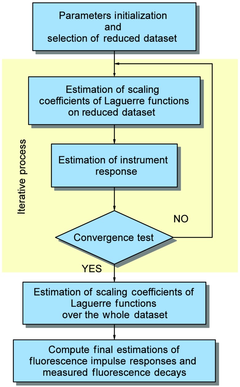
Finally, by considering the NNLSA in Eq. (30) for the scaling coefficients due to its faster implementation compared to CLSE in Eq. (29), and the closed-form solution for the instrument response in Eq. (37), the overall BDE algorithm is outlined next (see Fig. 2).

Fig. 2.

Block diagram of blind deconvolution estimation.

• I.Initialization and Selection of Reduced Dataset: Provide the FLIM measurements matrix $\mathbf{Y}$ and based on the selected spatial downsampling $D$, the reduced dataset $\widehat{\mathbf{Y}}$ is constructed. Define the number of samples to be estimated from the instrument response $\widehat{L}$ and its initial condition ${\theta }^0$, a maximum number of iterations $t_{\max }$, a convergence threshold for the estimation error $\kappa$, and the basis functions ${\{b_n[l]\}}_{n=0}^{N-1}$ to construct $\mathbf{B}$. Set $t=0$ and $J^0={10}^6$. From ${\theta }^0$, compute the input matrix ${\mathbf{U}}^0$ from Eq. (4).
• II.Estimation of Scaling Coefficients of Laguerre Functions: Set $t=t+1$, and for the reduced set of spatial locations $k\in [0,\widehat{K}-1]$ with ${\mathbf{U}}^{t-1}$, compute the NNLSA for ${\mathbf{c}}_k^t$ in Eqs. (30) and (31). Construct the resulting scaling coefficients matrix ${\mathbf{C}}^t$ in Eq. (15).
• III.Estimation of Instrument Response: Fixing ${\mathbf{C}}^t$, evaluate the optimal input parameters ${\theta }^t$ from Eq. (37). The resulting input matrix ${\mathbf{U}}^t$ is obtained from Eq. (18).
• IV.Convergence Test: Calculate the estimation error at $t$ stage as $J^t={\Vert \mathbf{Y}-{\mathbf{U}}^t{\mathbf{BC}}^t\Vert }_F$, and evaluate the error improvement $\mathrm{\Delta }{J}^t=|J^t-J^{t-1}|$ with respect to the previous iteration $t-1$. If $\mathrm{\Delta }{J}^t>\kappa$ and $t\le t_{\max }$ go to II, otherwise continue.
• V.Estimation of Scaling Coefficients of Laguerre Functions on the Whole Dataset: For the complete set of locations $k\in [0,K-1]$ with ${\mathbf{U}}^t$, compute the NNLSA for ${\mathbf{c}}_k^t$ in Eqs. (30) and (31).
• VI.
  Compute Final Estimations of Fluorescence Impulse Responses and Measured Fluorescence Decays: If we assume that the algorithm stops at $\widehat{t}$’th iteration with outputs $({\theta }^{\widehat{t}},{\mathbf{C}}^{\widehat{t}})$, the final estimations are given by

  $$\begin{gathered} \widehat{u}[l]=\{\begin{array}{ll}{\theta }_l^{\widehat{t}},& 0\le l\le \widehat{L}-1\\ 0,& \widehat{L}\le l\le L-1\end{array}, \\ {\widehat{\mathbf{h}}}_k={\mathbf{BC}}^{\widehat{t}}\Rightarrow {\widehat{h}}_k[l]=\sum _{n=0}^{N-1}{c}_{k,n}^{\widehat{t}}{b}_n[l]\forall l\in [0,L-1],k\in [0,K-1], \\ {\widehat{\mathbf{y}}}_k={\mathbf{U}}^{\widehat{t}}{\mathbf{BC}}^{\widehat{t}}\Rightarrow {\widehat{y}}_k[l]=\sum _{n=0}^{N-1}{c}_{k,n}^{\widehat{t}}\widehat{u}[l]\star b_n[l], \end{gathered}$$ (38)

  where the input matrix ${\mathbf{U}}^{\widehat{t}}$ is constructed from ${\theta }^{\widehat{t}}$ according to Eq. (4).

5. Synthetic and Experimental Validation

This section presents the validation of the BDE algorithm by considering two cases: synthetic and experimental FLIM datasets. For both cases, the estimation errors on the instrument response and measured fluorescence decays will be evaluated, and in the synthetic experiments, we also quantify the error on the resulting fluorescence impulse responses. In addition, the error on four different initial conditions in the instrument response will be analyzed, as well as different scenarios for shot noise in the synthetic fluorescence decays.³⁴ Meanwhile, in the experimental evaluation, we consider a comparison for different values of the spatial downsampling factor in step II of BDE, and a quantification of the lifetime in the fluorescence impulse responses. We point out that in the FLIM literature there is no other algorithm able to perform blind deconvolution that could provide a comparison benchmark.

5.1. Synthetic Evaluation

The synthetic dataset was generated by considering the measured instrument response in Ref. 7 with a sampling interval $T=250\mathrm{ps}$ and a length of 256 samples ($L=256$). This signal $u[l]$ has a sharp rising time and a subsequent exponential decay (see top plots in Fig. 4), and its normalized to sum 1, i.e., $\sum _{l}u[l]=1$ (assumption 1 in Sec. 2). The fluorescence impulse response at each spatial point $k$ is modeled as a sum of three exponential functions:

$$h_k[l]=\sum _{i=1}^3{a}_{k,i}{e}^{-l\frac{T}{{\tau }_{k,i}}}\forall k\in [0,K-1],l\in [0,L-1],$$ (39)

where the magnitudes and characteristic times of these functions are randomly chosen for any spatial point, i.e., $a_{k,i}\sim \mathcal{U}[0,50]$ and ${\tau }_{k,i}\sim \mathcal{U}[0.01,6]\mathrm{ns}$ $\forall k,i$. Next, the synthetic uncorrupted fluorescence decays $y_k^o[l]$ are computed by applying the convolution operator in Eq. (1), i.e., $y_k^o[l]=u[l]\star h_k[l]$. In our evaluation, we included shot noise in the measurements to take into account uncertainty in the equipment according to the following model:³⁴

$$y_k[l]=y_k^o[l]+\sqrt{y_k^o[l]}·{\omega }_k[l]\forall l\in [0,L-1],$$ (40)

where ${\omega }_k[l]\sim \mathcal{N}(0,{\sigma }_k^2)$ represents a normal random variable, and its variance ${\sigma }_k^2$ is selected with respect to a desired peak signal-to-noise ratio (PSNR),

$$\mathrm{PSNR}=10{\log }_{10}\frac{{\max }_{l\in [0,L-1]}{y}_k^o[l]}{{\sigma }_k^2}\forall k\in [0,K-1].$$ (41)

Fig. 4.

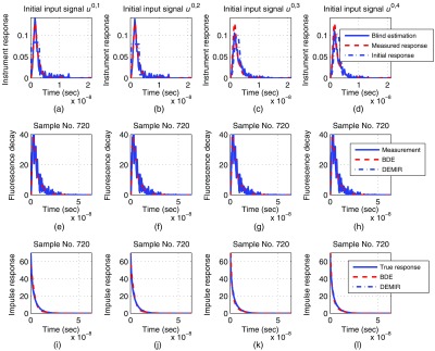
Synthetic evaluation at peak signal-to-noise ratio $(\mathrm{PSNR})=15\mathrm{dB}$, where each column corresponds to the initial instrument response $(u^{0,1},u^{0,2},u^{0,3},u^{0,4})$: (a)-(d) comparison for the instrument response estimation, (e)-(h) comparison for the fluorescence decay estimation at sample 720, (i)-(l) comparison for the fluorescence impulse response estimation at sample 720.

By assuming that $\widehat{u}[l]$, ${\widehat{h}}_k[l]$ and ${\widehat{y}}_k[l]$ denote the estimations by the BDE algorithm in Eq. (38), we compute three performance metrics to evaluate the accuracy of the methodology over the whole dataset:

$$\begin{gathered} E_u=\frac{\sum _{l=0}^{L-1}{(u[l]-\widehat{u}[l])}^2}{\sum _{l=0}^{L-1}{(u[l])}^2} \\ {E}_h=\frac{\sum _{k=0}^{K-1}\sum _{l=0}^{L-1}{(h_k[l]-{\widehat{h}}_k[l])}^2}{\sum _{k=0}^{K-1}\sum _{l=0}^{L-1}{(h_k[l])}^2} \\ {E}_y=\frac{\sum _{k=0}^{K-1}\sum _{l=0}^{L-1}{(y_k[l]-{\widehat{y}}_k[l])}^2}{\sum _{k=0}^{K-1}\sum _{l=0}^{L-1}{(y_k[l])}^2}. \end{gathered}$$ (42)

These three indices $(E_u,E_h,E_y)$ will give an indication of the weight of the error energy with respect to the estimated instrument response, fluorescence impulse responses, and measured fluorescence decays in a percentage fashion. Since the construction of the synthetic datasets involved random samples, we carry out a Monte Carlo evaluation by implementing the BDE algorithm according to the parameters listed in Table 1, whose selection is explained next. For the Laguerre functions,^17,18 the order of the approximation was set to 8th for the fluorescence impulse responses ($N=8$), and their shape parameter was selected as $\alpha =0.85$ by a trial and error method. Nonetheless, the two parameters $N=8$ and $\alpha =0.85$ were pretty robust throughout our whole validation stage, since we did not have to modify them for the synthetic and experimental scenarios, although they represent different types of FLIM datasets. In the synthetic evaluation, 3600 spatial samples were generated by Eqs. (39) and (40) at different PSNRs (15, 20, 25, and 30 dB), and the resulting datasets were analyzed by the BDE algorithm, i.e., $K=3600$. The spatial downsampling inside the iterative process at step II of the BDE was set to $D=8$, i.e., only $\widehat{K}=K/D=450$ spatial samples were employed to estimate the instrument response. In our evaluation, this reduced number of measurements $\widehat{K}$ was low enough to minimize the complexity in the estimation of the instrument response, but still provided enough information to precisely reconstruct it. Meanwhile, the whole time evolution of the instrument response is captured in less than 13.75 ns, so we selected its estimated number of samples as $\widehat{L}=55$, which corresponds to this time by the assigned sampling interval $T$. Finally, to evaluate convergence in the iterative process of the BDE (see Fig. 2), we set the maximum number of iterations as $t_{\max }=20$ and the convergence precision as $\kappa =0.01$, as a good balance between precision and complexity in our evaluations. All the data processing was carried out in MATLAB^®. In order to study the performance under different initialization signals, four prototypes were chosen according to the mean spatial measurement in the dataset:

$$y^m[l]=\left(\frac{1}{\mathit{K}}\right)\underset{}{\overset{}{{\sum }_{k=0}^{\mathit{K}-1}}}{y}_k[l]\forall l\in [0,L-1],$$ (43)

and its energy $\mathrm{\Gamma }=\sum _{l=0}^{L-1}{(y^m[l])}^2$. The initial instrument responses $(u^{0,1},u^{0,2},u^{0,3},u^{0,4})$ are analytically described by

$$u^{0,1}[l]=\{\begin{array}{ll}1,& l\in {\mathcal{I}}_1\\ 0,& \text{elsewhere}\end{array},$$ (44)

$$u^{0,2}[l]=\{\begin{array}{cc}1,& l\in {\mathcal{I}}_1\\ 0.1,& l\in {\mathcal{I}}_2\\ 0,& \text{elsewhere}\end{array},$$ (45)

$$u^{0,3}[l]=\{\begin{array}{ll}{y}^{m,1}[l],& l\in [0,I_{\max }]\\ y^{m,2}[(l-I_{\max }-1)·\eta ],& l\in [I_{\max }+1,I_{\max }+1+(L-1-I_{\max }-1)/\eta ]\\ 0,& \text{elsewhere}\end{array},$$ (46)

$$u^{0,4}[l]=\{\begin{array}{ll}{y}^{m,1}[l],& l\in [0,I_{\max }]\\ y^{m,1}[2I_{\max }-l],& l\in [I_{\max }+1,2I_{\max }]\\ 0,& \text{elsewhere}\end{array},$$ (47)

where

$${\mathcal{I}}_1=\{l\in [0,L-1]|0<{(y^m[l])}^2/\mathrm{\Gamma }\le {\mathrm{\Omega }}_1\},$$ (48)

$${\mathcal{I}}_2=\{l\in [0,L-1]|{\mathrm{\Omega }}_1<{(y^m[l])}^2/\mathrm{\Gamma }\le {\mathrm{\Omega }}_2\},$$ (49)

$$I_{\max }=\arg \underset{l\in [0,L-1]}{\max }{y}^m[l],$$ (50)

$$y^{m,1}[l]=y^m[l]\forall l\in [0,I_{\max }],$$ (51)

$$y^{m,2}[l]=y^m[l+I_{\max }+1]\forall l\in [0,L-1-I_{\max }-1],$$ (52)

${\mathrm{\Omega }}_1,{\mathrm{\Omega }}_2\in (0,1)$, (${\mathrm{\Omega }}_1<{\mathrm{\Omega }}_2$), and $\eta \in \mathbb{Z}$ ($\eta >1$). In this way, ${\mathcal{I}}_1$ and ${\mathcal{I}}_2$ are the sets of time indices such that the energy of the mean spatial fluorescence decay measurement $y^m[l]$ is below ${\mathrm{\Omega }}_1$%, and between ${\mathrm{\Omega }}_1$% and ${\mathrm{\Omega }}_2$% of its maximum value, respectively; $I_{\max }$ is the time index for the peak value in the mean measurement; and $y^{m,1}[l]$ and $y^{m,2}[l]$ are the extracted signals below and above the peak mean measurement, respectively. In this way, the initial instrument responses take the following shapes:

Table 1.

Parameters of synthetic dataset and blind deconvolution estimation (BDE) implementation during the synthetic evaluation.

Parameter	Value
$T_s$	0.250 ns
$K$	3600
$L$	256
$\widehat{L}$	55
$D$	8
$N$	8
$\alpha$	0.85
$t_{\max }$	20
$\kappa$	0.01

• •$u^{0,1}$ represents a square pulse with time duration of ${\mathrm{\Omega }}_1$% the energy of the mean fluorescence decay;
• •$u^{0,2}$ describes a two-step staircase signal with first-step duration of ${\mathrm{\Omega }}_1$% the energy of the mean fluorescence decay, and second-step time length between ${\mathrm{\Omega }}_1$% and ${\mathrm{\Omega }}_2$%;
• •$u^{0,3}$ stands for an asymmetric pulse generated by the mean fluorescence decay until its peak value, and its downsampled version²⁸ by $\eta$ factor above the peak; and
• •$u^{0,4}$ depicts a symmetric pulse generated by the mean fluorescence decay until its peak value, and its reflection from this position.

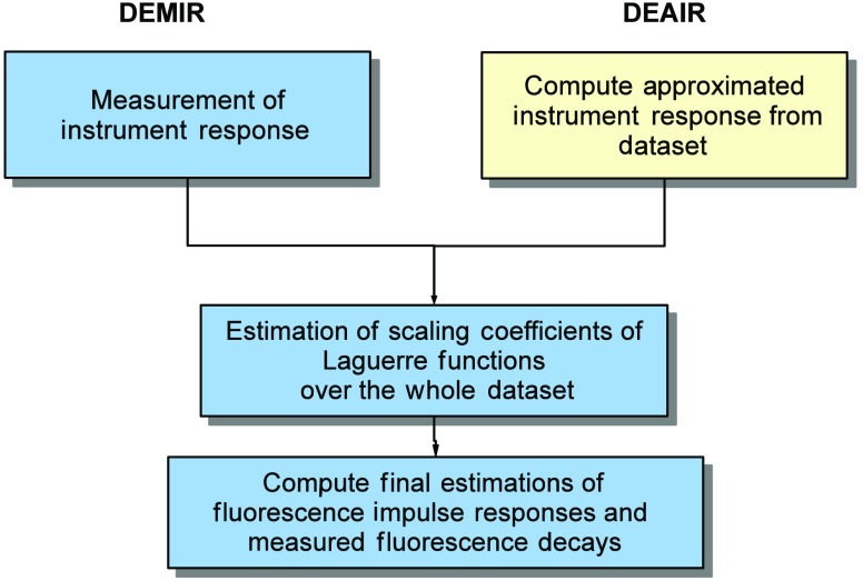
Therefore, the construction of $(u^{0,1},u^{0,2})$ mainly depends on the time energy distribution of the mean fluorescence decay, and $(u^{0,3},u^{0,4})$ on its increasing and decreasing patterns with respect to its peak value. In our evaluation, the free parameters were set to the values ${\mathrm{\Omega }}_1=0.35$, ${\mathrm{\Omega }}_2=0.7$, and $\eta =5$ by a trial and error procedure. These four initial instrument responses $(u^{0,1},u^{0,2},u^{0,3},u^{0,4})$ were later normalized by the condition in Eq. (3). In addition, our evaluation also considers the deconvolution estimation with measured instrument response (DEMIR) $u[l]$ by applying the NNLSA in Eq. (30) (see Fig. 3). Hence, two new performance indices $E_h^0$ and $E_y^0$ can examine the estimation accuracy in the fluorescence impulse response and measured fluorescence decays by a direct deconvolution process. Therefore, $E_h^0$ and $E_y^0$ are the two lower bounds in the performance of the BDE algorithm for the four initial conditions $(u^{0,1},u^{0,2},u^{0,3},u^{0,4})$.

Fig. 3.

Block diagram of deconvolution with measured instrument response and deconvolution with approximated instrument response.

Table 2 presents the results of our synthetic evaluation and shows that the choice of the initial condition has a small effect on the resulting estimation performance $(E_u,E_h,E_y)$ for BDE. In the experiments, $u^{0,1}$ and $u^{0,2}$ consistently achieved the best estimations for the instrument and fluorescence impulse responses $(E_u,E_h)$ at all PSNR values. On the other hand, there were no significant performance differences in the estimation in the output intensity $E_y$ for all initial responses. Overall, for all initial conditions $(u^{0,1},u^{0,2},u^{0,3},u^{0,4})$, the performance is comparable among the metrics in Eq. (42), since the best-case and worst-case errors for the instrument and fluorescence impulse response estimations $(E_u,E_h)$ were 11%–26%, and 8.5%–26%, respectively. Meanwhile, the estimation error for the fluorescence decay $E_y$ varied in a smaller range of 1–5% for all initial conditions. Consequently, the approximations were more precise with respect to the measured fluorescence decays, which provided smaller estimation errors $E_y$ compared to $(E_u,E_h)$. The lower bounds $(E_h^0,E_y^0)$ based on DEMIR for the fluorescence impulse response and measured fluorescence decay had also little variations as 4–7% and 1–5%, respectively. In fact, the performance results $(E_h,E_y)$ for BDE with the initial instrument responses $u^{0,1}$ and $u^{0,2}$ were comparable to DEMIR in $(E_h^0,E_y^0)$, which is its lower bound. Another important property is that the performance metrics were lightly influenced by the PSNR, where the instrument response and fluorescence impulse response estimations $(E_u,E_h)$ were the mostly sensible metrics. Nonetheless, the general trend was that as the PSNR increased, the resulting errors $(E_u,E_h,E_y)$ had a small decrease for all initial conditions $(u^{0,1},u^{0,2},u^{0,3},u^{0,4})$. Figure 4 illustrates the resulting input estimations by the BDE algorithm for a PSNR = 15 dB and sample 720, where as expected, all the initial points qualitatively provided good results. Also, this figure presents a sample of the estimated fluorescence decays and impulse responses for the three initial instrument responses $(u^{0,1},u^{0,2},u^{0,3},u^{0,4})$. These plots illustrate a good fit to the synthetic data.

Table 2.

Performance quantification of synthetic datasets for BDE and deconvolution estimation with measured instrument response (DEMIR) with different initial instrument responses and peak signal-to-noise ratios (PSNRs).

PSNR (dB)	BDE				DEMIR
	$E_u$				—
	$u^{0,1}$	$u^{0,2}$	$u^{0,3}$	$u^{0,4}$
15	0.1684	0.1627	0.2559	0.2186
20	0.1470	0.1241	0.2149	0.1782
25	0.1416	0.1286	0.2033	0.1754
30	0.1165	0.1062	0.1636	0.1419
PSNR (dB)	$E_h$				$E_h^0$
	$u^{0,1}$	$u^{0,2}$	$u^{0,3}$	$u^{0,4}$
15	0.0849	0.0848	0.2605	0.2057	0.0663
20	0.0985	0.0856	0.2209	0.1730	0.0515
25	0.1029	0.0954	0.2050	0.1696	0.0482
30	0.0897	0.0836	0.1574	0.1315	0.0443
PSNR (dB)	$E_y$				$E_y^0$
	$u^{0,1}$	$u^{0,2}$	$u^{0,3}$	$u^{0,4}$
15	0.0470	0.0470	0.0470	0.0470	0.0466
20	0.0264	0.0263	0.0264	0.0263	0.0261
25	0.0151	0.0148	0.0202	0.0190	0.0146
30	0.0121	0.0120	0.0153	0.0146	0.0105

5.2. Experimental Evaluation

5.2.1. Ex vivo atherosclerotic plaques datasets

The first experimental evaluation considers the analysis of multispectral FLIM (m-FLIM) datasets of ex vivo atherosclerotic plaques.⁷ The temporal resolution of the measurements is 250 ps. All the measurements include three wavelength bands: $390\pm 20$, $452\pm 22.5$, and $550\pm 20$ nm. Each effective time trace has a total of $L=167$ samples per wavelength. Sixty individual datasets with $60\times 60$ spatial samples were analyzed by the BDE algorithm to estimate the instrument and fluorescence impulse responses and measured fluorescence decays. The same parameters employed in the synthetic evaluation of BDE were considered for the experimental datasets (see Table 1). Since each m-FLIM measurement considers three wavelengths, we only analyze the third wavelength, which has distinct information for classification purposes, i.e., a total of $K=3600$ spatial points for deconvolution. For all datasets, the instrument response has the same time-domain characteristics and it was recorded for comparison purposes in order to apply DEMIR. Meanwhile, the instrument response is often approximated as a pulse created from the rising part of the measured fluorescence decay by mirroring it around the peak of the fluorescence decay pulse, similar to the initial input response $u^{0,4}$ in Eq. (47). This approximated instrument response (AIR) pulse is also used for deconvolution in the experimental evaluation. The deconvolution by using the AIR pulse is defined as deconvolution estimation with approximated instrument response (DEAIR), and it involves the solution of NNLSA in Eq. (30) for all 60 datasets (see Fig. 3). These comparison strategies, DEMIR and DEAIR, are both based on a Laguerre-base deconvolution, so they employ the same expansion order $N$ and shape parameter $\alpha$ as in BDE (see Table 1).

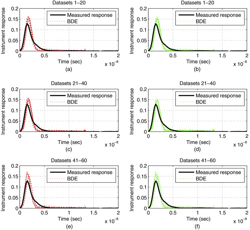
In this experimental evaluation, we will study the effect of modifying the spatial downsampling that is used to obtain the reduced set of measurements $\widehat{\mathbf{Y}}$. We will consider two cases, $D=8$ and $D=36$, i.e., $\widehat{K}=3600/8=450$ and $\widehat{K}=3600/36=100$ spatial samples are used to reconstruct the instrument response at step II of BDE. Figure 5 qualitatively compares the estimated instrument responses for the 60 datasets by considering $u^{0,1}$ as the initial condition, and both spatial downsampling factors ($D=8$ and $D=36$). As a result, a good estimation is visualized for all datasets and values of $D$, although some minor discrepancies were observed. These small magnitude and pulse duration differences in the estimations of Fig. 5 are mainly due to noise in the FLIM dataset, since by the synthetic results in the previous section (see Table 2), a perfect reconstruction of the instrument response will require a large PSNR. Nonetheless, these magnitude errors did not affect the fluorescence impulse response estimations, as the next statistical analysis will show. Next, the shape of the instrument response can be quantified by the full width at half maximum (FWHM) parameter, and in our experimental setup, the measured value was 1.53 ns. From the results in Fig. 5, the estimations by BDE produced a mean FWHM of 1.35 ns for $D=8$ and $D=36$, but the AIR pulse produced a large mean value of 2.08 ns. Thus, by comparing to the FWHM of the measured instrument response, the BDE estimation has a percentage error of 11.6%, and the AIR pulse of 36.2%. In this way, an advantage is visualized by BDE estimation compared to the AIR pulse.

Fig. 5.

Experimental evaluation for blind deconvolution estimation (BDE) with datasets of atherosclerotic plaques: comparison for the instrument response estimation for two spatial downsamplings (left column) $D=8$ and (right column) $D=36$, with (a, b) datasets 1–20, (c, d) datasets 21–40, (e, f) datasets 41–60.

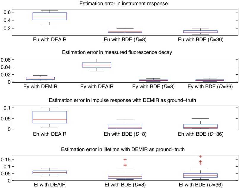
Figure 6 (top panels) illustrates the boxplots for the metrics $E_u$ and $E_y$ with the BDE algorithm, and considering DEAIR. As expected, the instrument response estimation by DEAIR presents a larger error compared to BDE. For the 60 datasets, the mean value of $E_u$ was 11–12% for BDE with both spatial downsamplings, and 49% for DEAIR. Figure 6 (second row) illustrates the estimation error for the measured fluorescence decay $E_y$ by using DEMIR. These results show no significant differences in the DEMIR and BDE output estimation performances with $D=8$ and $D=36$, although there is a strong difference with DEAIR (see second panel in Fig. 6). The mean value of $E_y$ was 1% for DEMIR and 0.4% for BDE with both spatial downsamplings, and 4.5% for DEAIR. Hence, the BDE method achieved more accurate estimations of the FLIM measurements than with the measured instrument response. These statistical results corroborate the qualitative performance of Fig. 5, which illustrates a good estimation for the instrument response, since as previously remarked, the pulse shape of the input excitation is correctly estimated. In addition, the third panel of Fig. 6 shows the estimation error in the fluorescence impulse response $E_h$ in Eq. (42) by taking as a ground truth the DEMIR approximation. Hence, the BDE provides closer estimations to DEMIR, since the mean error for all datasets was 1.3% ($D=8$ and $D=36$), but for DEAIR the mean error rose to 5.4%. Finally, if ${\widehat{\mathbf{h}}}_k^{\ell }\in {\mathbb{R}}^L$ represents the approximated fluorescence impulse response vector at $k$’th spatial sample by $\ell$ strategy $(\ell \in \{\mathrm{DEMIR},\mathrm{DEAIR},\mathrm{BDE}\})$, and ${\mathbf{t}}_k\in {\mathbb{R}}^L$ the vector of time samples, the lifetime of the time response ${\lambda }_k$ can be computed as³⁴

$${\lambda }_k^{\ell }=\frac{{\mathbf{t}}_k^{\top }{\widehat{\mathbf{h}}}_k^{\ell }}{{\mathbf{1}}_L^{\top }{\widehat{\mathbf{h}}}_k^{\ell }}\forall k\in [0,K-1].$$ (53)

Thus, by assuming that the lifetime by DEMIR is the ground truth, the percentage error in the estimation by DEAIR and BDE over the whole dataset is defined as

$$E_l^{\mathrm{DEAIR}}=\frac{1}{K}\sum _{k=0}^{K-1}\frac{|{\lambda }_k^{\mathrm{DEMIR}}-{\lambda }_k^{\mathrm{DEAIR}}|}{{\lambda }_k^{\mathrm{DEMIR}}},$$ (54)

$$E_l^{\mathrm{BDE}}=\frac{1}{K}\sum _{k=0}^{K-1}\frac{|{\lambda }_k^{\mathrm{DEMIR}}-{\lambda }_k^{\mathrm{BDE}}|}{{\lambda }_k^{\mathrm{DEMIR}}}.$$ (55)

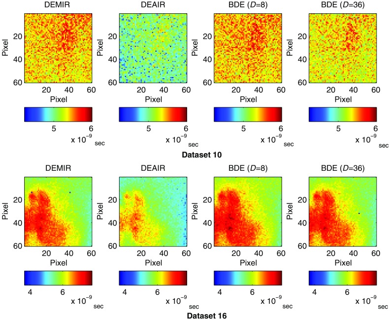
Thus, the last panel in Fig. 6 presents the results for $E_l^{\mathrm{DEAIR}}$ and $E_l^{\mathrm{BDE}}$, where once more BDE provided the best estimation. The mean lifetime estimation error over the 60 datasets was 6.4% by DEAIR, and this value was reduced to 3.4% and 4% for BDE with $D=8$ and $D=36$, respectively. Figure 7 presents the resulting lifetime images for datasets 10 and 16 with DEMIR, DEAIR, and BDE ($D=8$ and $D=36$). The resulting lifetime images highlight a good agreement between DEMIR and BDE, independently of the spatial downsampling. Consequently, once more, the large reduction in the FLIM measurements used to estimate the instrument response did not produce a significant loss of accuracy in the BDE algorithm. However, DEAIR shows some important differences for both datasets, which confirms the advantage of BDE in the deconvolution and lifetime estimation processes.

Fig. 6.

Experimental evaluation with datasets of atherosclerotic plaques: boxplot results for the metrics $E_u$ and $E_y$ by deconvolution estimation with approximated instrument response (DEAIR) and BDE with spatial downsampling of 8 and 36, $E_y$ by deconvolution estimation with measured instrument response (DEMIR), and $E_h$ and $E_l$ by DEAIR and BDE taking the results by DEMIR as ground truth.

Fig. 7.

Experimental evaluation for datasets 10 and 16 of atherosclerotic plaques: lifetimes images that employ the estimations by DEMIR, DEAIR, and BDE with spatial downsamplings of 8 and 36.

On the other hand, Table 3 presents the average computational time per FLIM dataset in the MATLAB implementation for the lifetime estimation by using a Pentium Intel Core i7-4770 3.5 GHz quad-core processor and 32 GB RAM computer. This table also shows the average computational time of just the blind approximation of the instrument response for each dataset, so the effect of the spatial downsampling can be clearly observed in BDE. Hence, the spatial downsampling provided some reduction in the computational time without compromising the accuracy of the estimations, as shown in Fig. 6. Thus, to obtain the lifetime image of each dataset, the BDE required in average 11.22 s for a spatial downsample of 36 ($D=36$), and just 6.53 s to estimate the instrument response. Meanwhile, as expected, the fastest lifetime estimation is achieved by DEMIR since its implementation requires just a direct computation of NNLSA in Eq. (30). The next fastest estimation is DEAIR due to the initial basic approximation of the instrument response based on the mean FLIM measurements. Nevertheless, the extra computation time by BDE compared to DEAIR is justified to achieve more accurate approximations of the instrument response, fluorescence impulse responses, and lifetimes in general.

Table 3.

Computational time by DEMIR, deconvolution estimation with approximated instrument response (DEAIR) and BDE ($D=8$ and $D=36$) for overall lifetime evaluation and blind instrument response estimation during experimental tests with 60 datasets of atherosclerotic plaques.

	Computational time
	Overall lifetime estimation				Instrument response estimation
	DEMIR	DEAIR	BDE		BDE
			$(D=8)$	$(D=36)$	$(D=8)$	$(D=36)$
Mean	1.47 s	2.59 s	13.42 s	11.58 s	6.94 s	6.71 s
Standard deviation	0.27 s	0.19 s	5.61 s	4.38 s	2.05 s	2.36 s

5.2.2. Human breast cancer cell datasets

The last experimental evaluation consists of processing fluorescence lifetime images of 13 human breast cancer cell samples used to measure metabolic inhibition by cyanide treatment.¹² The fluorescence images were captured by a custom-built multiphoton microscope (Prairie Technologies). Since the primary target is to quantify the fluorescence response of coenzymes nicotinamide adenine dinucleotide (NADH) and flavin adenine dinucleotide (FAD), there are two optic excitations: one tuned to 750 nm for NADH excitation and another one to 890 nm for FAD excitation. To isolate the response to NADH and FAD, there are two bandpass filters: $440\pm 40\mathrm{nm}$ (NADH) and $550\pm 50\mathrm{nm}$ (FAD). Each pixel has a dwell time of $4.8\mu \mathrm{s}$ to acquire images of dimension $256\times 256$. The fluorescence lifetime image for each optic excitation was collected using time-correlated single-photon counting electronics, where the instrument response FWHM was 260 ps for both laser excitations. In this test bench, the temporal resolution of the measurements is 49 ps, and the length of the time responses is 175 and 190 samples for the first and second wavelengths, respectively.

The parameters of the BDE were the same as in the previous experimental evaluation (see Table 1), where the spatial downsample was set to 36 $(D=36)$. Compared to the initial experimental validation, now there are two different optic excitations, one per each studied wavelength and they were both estimated in our analysis. Since not all the pixels in the sample image contain relevant information, the pixels with low energy were masked. For this purpose, a stacked vector with the fluorescence decay responses at both wavelengths for each pixel was constructed, and its Euclidean norm was computed. The peak value of the Euclidean norm in the image was identified, and if the ratio between the norm of the stacked responses at a given pixel and the peak value is below 5%, the pixel is masked to avoid further processing.

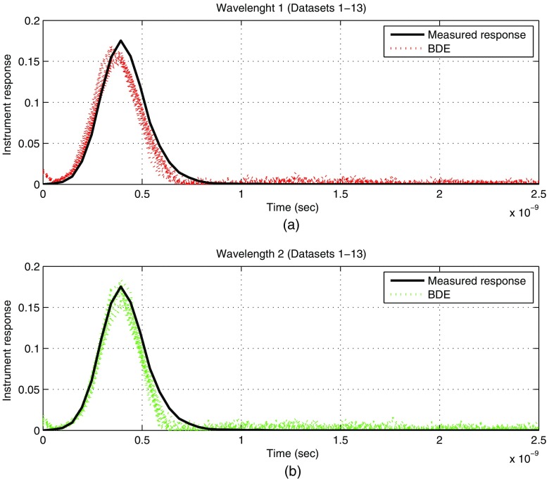
For the 13 datasets, the estimated instrument responses per wavelength were computed by the BDE and quantified by the FWHM parameter. The mean FWHM for wavelength 1 was 258 ps, and for wavelength 2 was 234 ps. As a result, by considering that the measured FWHM is 260 ps, a good estimation is achieved by our blind algorithm. The estimated 13 instrument responses for both wavelengths are plotted against the measured response in Fig. 8. Thus, a small error is observed for both conditions, where the shape of the instrument response is well captured by the BDE, although with some minor magnitude and pulse duration adjustments. As in the case of the FLIM datasets of atherosclerotic plaques, the magnitude and pulse duration differences in the estimations of Fig. 8 could be reduced at a cost of large PSNRs in the whole dataset. As previously described, these datasets have regions with low energy near the boundary of the processing mask, so the resulting PSNRs are low at these areas and this condition slightly affects the instrument response estimations.

Fig. 8.

Experimental evaluation with datasets of human breast cancer cell samples: estimated instrument responses per wavelength: (a) wavelength 1 (datasets 1–13) and (b) wavelength 2 (datasets 1–13).

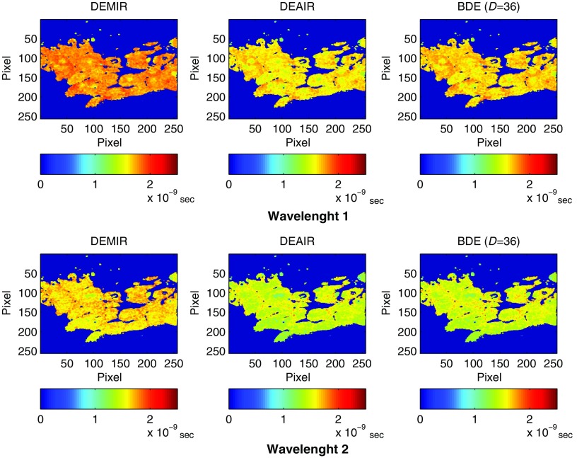
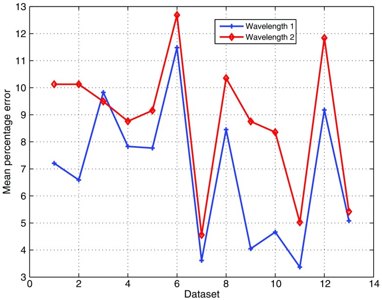
The lifetimes were next computed by the BDE from the estimated fluorescence impulse responses. For comparison, the fluorescence impulse responses were also estimated by DEMIR and DEAIR for the same parameters in the Laguerre expansion (see Table 1). The estimated lifetime by DEMIR is labeled as the ground truth. Figure 9 illustrates the lifetimes for dataset 1 under the three approaches (DEMIR, DEAIR, and BDE), where a good agreement is observed by our blind technique in both wavelengths. Meanwhile, DEAIR presents, in general, lower lifetime estimations compared to BDE, which is consistent with our previous evaluation in Fig. 7. For all 13 datasets, the mean percentage error in the estimated lifetime by BDE was 6.9% in the first wavelength and 8.8% in the second wavelength. Figure 10 shows the mean percentage error for each dataset for both wavelengths, where as pointed out earlier, the estimated lifetime by DEMIR is considered the reference point. This plot confirms the accuracy of the BDE, since the worst-case mean percentage error is below 13% for any wavelength, and the best response has an error of just 3.4%. Hence, despite the fact that our algorithm does not rely on any prior information of the instrument response in the system, the BDE provided good estimations of the lifetimes for the FLIM datasets. Compared to the mean lifetime estimation errors for the atherosclerotic plaques FLIM datasets by BDE ($\approx 4\%$), the percentage errors slightly increased in this case to $\approx 9\%$. We believe that this effect is due to two main aspects: the FLIM instrumentation is different, so the noise properties are not comparable, and the FLIM datasets of breast cancer cell samples have regions of low PSNR near the processing mask. Hence, we believe that FLIM datasets with heterogeneous and low PSNRs might affect the lifetime estimations.

Fig. 9.

Experimental evaluation with dataset 1 of human breast cancer cell samples: estimated lifetime by BDE (first column) and DEMIR (second column) for both wavelengths.

Fig. 10.

Experimental evaluation with datasets of human breast cancer cell samples: mean percentage error in the estimated lifetime of the fluorescence impulse response for both wavelengths by BDE.

6. Conclusions

This paper proposes a method, denoted as BDE, to solve the problem of blind deconvolution for FLIM data. A linear combination of basis functions models the fluorescence impulse response at each spatial point. The BDE algorithm searches for the samples of the instrument response with a global perspective, meanwhile the scaling coefficients of the basis functions are computed for each point in the sample. The core of the BDE algorithm is an ALS methodology that iteratively estimates the decision variables. The recurrent steps in the BDE algorithm rely on constrained quadratic programming and least-squares solutions. During this iterative process, just a reduced set of measurements is employed to speed up the convergence. After convergence, the BDE method provides an estimation of the instrument response. In the final step of the proposed methodology, the BDE algorithm computes the scaling coefficients of the fluorescence impulse response over the whole dataset. Our synthetic and experimental results showed that the proposal is robust to uncertainty in the measured fluorescence decays and variations in the initial input condition. As a future work, the blind estimation of the instrument response will be used as the initial step for deconvolution techniques based on multiexponential models. In addition, besides Laguerre functions, different basis will be also explored for the fluorescence impulse response, and a toolbox in MATLAB will be developed to facilitate the final user interaction.

Biographies

Daniel U. Campos-Delgado has been a professor at the Universidad Autonoma de San Luis Potosi (UASLP) in Mexico since 2001. He received his BS degree in electronics engineering from UASLP in 1996, and his MSEE and PhD degrees from Louisiana State University, Baton Rouge, USA, in 1999 and 2001, respectively. He is the author of more than 150 referred papers in scientific journals and congresses. His current research interests include optimization, dynamic modeling, and optimal signal processing.

Omar Gutierrez-Navarro is an assistant professor at the Universidad Autonoma de Aguascalientes, Mexico. He received his BS degree in electronics engineering from Universidad Autonoma de San Luis Potosi (UASLP), his MSc degree in computer science and industrial mathematics from the Center for Research in Mathematics in Guanajuato, Mexico, in 2007, and his PhD degree in electronics engineering from UASLP in 2014. His research interests include numerical methods for characterization of living tissue using fluorescence lifetime imaging microscopy data.

Edgar R. Arce-Santana is a professor at the Universidad Autonoma de San Luis Potosi in Mexico. He received his BS degree in computer science from the Technological Institute of San Luis Potosi in 1987 and his MSc and PhD degrees from the Center for Research in Mathematics in Guanajuato, Mexico, in 2000 and 2004, respectively. He is the author of more than 50 referred papers in scientific journals and congresses. His current research interests include computer vision, optimization, signal processing, and pattern recognition.

Melissa C. Skala is an assistant professor of biomedical engineering at Vanderbilt University. She received her BS degree in physics from Washington State University in 2002 her MS degree in biomedical engineering from the University of Wisconsin, Madison, in 2004, and her PhD in biomedical engineering from Duke University in 2007. Her primary research interests include nonlinear microscopy, metabolic imaging, optical coherence tomography, hyperspectral imaging, photothermal imaging, nanophotonics, cancer, and cardiovascular disease.

Alex J. Walsh is a postdoctoral fellow at the Air Force National Research Lab in San Antonio, Texas. She received her BE, MS, and PhD degrees in biomedical engineering from Vanderbilt University in 2010, 2012, and 2015, respectively. Her research interests include nonlinear microscopy and photon-tissue interactions.

Javier A. Jo is an associate professor of biomedical engineering at Texas A&M University. He received his BS degree in electrical engineering from the Pontificia Universidad Catolica del Peru in 1996 and his MS and PhD degrees from the University of Southern California, Los Angeles, in 2000 and 2002, respectively. His primary research interests include systems analysis, signal and image processing, and biomedical instrumentation, with applications to biophotonics, physiology, and medicine.

References

- 1.Marcu L., French P. M. W., Elson D. S., Fluorescence Lifetime Spectroscopy and Imaging: Principles and Applications in Biomedical Diagnostics, CRC Press, Boca Raton, Florida: (2014). [Google Scholar]
- 2.Anthony N., Berland K., Guo P., “Principles of fluorescence for quantitative fluorescence microscopy,” in FLIM Microscopy in Biology and Medicine, Periasamy Ammasi, Clegg Robert M., Eds., pp. 35–63, Chapman and Hall/CRC, Boca Raton, Florida: (2009). [Google Scholar]
- 3.Periasamy A., Clegg R. M., FLIM Microscopy in Biology and Medicine, Chapman and Hall/CRC, Boca Raton, Florida: (2009). [Google Scholar]
- 4.Lakowicz J. R., Principles of Fluorescence Spectroscopy, Springer, New York: (2006). [Google Scholar]
- 5.Shrestha S., et al. , “High-speed multispectral fluorescence lifetime imaging implementation for in vivo applications,” Opt. Lett. 35, 2558–2560 (2010). 10.1364/OL.35.002558 [DOI] [PMC free article] [PubMed] [Google Scholar]
- 6.O’Donnell M., et al. , “Multimodality cardiovascular molecular imaging technology,” J. Nucl. Med. 51(Suppl. 1), 38S–50S (2010). 10.2967/jnumed.109.068155 [DOI] [PMC free article] [PubMed] [Google Scholar]
- 7.Park J., et al. , “Biochemical characterization of atherosclerotic plaques by endogenous multispectral fluorescence lifetime imaging microscopy,” Atherosclerosis 220(2), 394–401 (2012). 10.1016/j.atherosclerosis.2011.10.034 [DOI] [PMC free article] [PubMed] [Google Scholar]
- 8.De Giorgi V., et al. , “Combined non-linear laser imaging (two-photon excitation fluorescence microscopy, fluorescence lifetime imaging microscopy, multispectral multiphoton microscopy) in cutaneous tumours: first experiences,” J. Eur. Acad. Dermatol. Venereol. 23(3), 314–316 (2009). 10.1111/j.1468-3083.2008.03045.x [DOI] [PubMed] [Google Scholar]
- 9.Galletly N., et al. , “Fluorescence lifetime imaging distinguishes basal cell carcinoma from surrounding uninvolved skin,” Br. J. Dermatol. 159(1), 152–161 (2008). 10.1111/j.1365-2133.2008.08577.x [DOI] [PubMed] [Google Scholar]
- 10.Jabbour J. M., et al. , “Fluorescence lifetime imaging and reflectance confocal microscopy for multiscale imaging of oral precancer,” J. Biomed. Opt. 18(4), 046012 (2013). 10.1117/1.JBO.18.4.046012 [DOI] [PMC free article] [PubMed] [Google Scholar]
- 11.Mycek M., Schomacker K., Nishioka N., “Colonic polyp differentiation using time-resolved autofluorescence spectroscopy?,” Gastrointest. Endosc. 48, 390–394 (1998). 10.1016/S0016-5107(98)70009-4 [DOI] [PubMed] [Google Scholar]
- 12.Walsh A. J., et al. , “Quantitative optical imaging of primary tumor organoid metabolism predicts drug response in breast cancer,” Cancer Res. 74(18), 5184–5194 (2014). 10.1158/0008-5472.CAN-14-0663 [DOI] [PMC free article] [PubMed] [Google Scholar]
- 13.Walsh A. J., et al. , “Optical metabolic imaging identifies breast cancer glycolytic levels, sub-types, and early treatment response,” Cancer Res. 73(20), 6164–6174 (2013). 10.1158/0008-5472.CAN-13-0527 [DOI] [PMC free article] [PubMed] [Google Scholar]
- 14.Lee B. K. C., et al. , “Application of the stretched exponential function to fluorescence lifetime imaging,” J. Biophys. 81(3), 1265–1274 (2001). 10.1016/S0006-3495(01)75784-0 [DOI] [PMC free article] [PubMed] [Google Scholar]
- 15.Pelet S., et al. , “A fast global fitting algorithm for fluorescence lifetime imaging microscopy based on image segmentation,” Biophys. J. 87, 2807–2817 (2004). 10.1529/biophysj.104.045492 [DOI] [PMC free article] [PubMed] [Google Scholar]
- 16.Warren S. C., et al. , “Rapid global fitting of large fluorescence lifetime imaging microscopy datasets,” PLoS One 8(8), e70687 (2013). 10.1371/journal.pone.0070687 [DOI] [PMC free article] [PubMed] [Google Scholar]
- 17.Jo J. A., et al. , “Fast model-free deconvolution of fluorescence decay for analysis of biological systems,” J. Biomed. Opt. 9(4), 743–752 (2004). 10.1117/1.1752919 [DOI] [PMC free article] [PubMed] [Google Scholar]
- 18.Dabir A. S., et al. , “Fully automated deconvolution method for on-line analysis of time-resolved fluorescence spectroscopy data based on an iterative Laguerre expansion technique,” J. Biomed. Opt. 14(2), 024030 (2009). 10.1117/1.3103342 [DOI] [PubMed] [Google Scholar]
- 19.Liu J., et al. , “A novel method for fast and robust estimation of fluorescence decay dynamics using constrained least-squares deconvolution with Laguerre expansion,” Phys. Med. Biol. 57, 843–865 (2012). 10.1088/0031-9155/57/4/843 [DOI] [PMC free article] [PubMed] [Google Scholar]
- 20.Fereidouni F., Bader A. N., Gerritsen H. C., “Spectral phasor analysis allows rapid and reliable unmixing of fluorescence microscopy spectral images,” Opt. Express 20(12), 12729–12741 (2012). 10.1364/OE.20.012729 [DOI] [PubMed] [Google Scholar]
- 21.Fereidouni F., Blab G. A., Gerritsen H. C., “Blind unmixing of spectrally resolved lifetime images,” J. Biomed. Opt. 18(8), 086006 (2013). 10.1117/1.JBO.18.8.086006 [DOI] [PubMed] [Google Scholar]
- 22.Mathews J. H., Fink K. K., Eds., Numerical Methods Using MATLAB, 4th ed., Prentice-Hall, Upper Saddle River, New Jersey: (2004). [Google Scholar]
- 23.Nocedal J., Wright S. J., Eds., Numerical Optimization, 2nd ed., Springer-Verlag, New York: (2006). [Google Scholar]
- 24.Seok J., Kim J., “Alternating minimization of the negative Poisson likelihood function for the global analysis of fluorescence lifetime imaging microscopy data,” Opt. Express 22(21), 24977 (2014). 10.1364/OE.22.024977 [DOI] [PubMed] [Google Scholar]
- 25.Jezierska A., et al. , “An EM approach for time-variant Poisson-Gaussian model parameter estimation,” IEEE Trans. Signal Process. 62(1), 17–30 (2014). 10.1109/TSP.2013.2283839 [DOI] [Google Scholar]
- 26.Young F. W., de Leeuw J., Takane Y., “Regression with qualitative and quantitative variables: an alternating least squares method with optimal features,” Psychometrika 41(4), 505–526 (1976). 10.1007/BF02296972 [DOI] [Google Scholar]
- 27.Jaumot J., et al. , “A graphical user-friendly interface for MCR-ALS: a new tool for multivariate curve resolution in MATLAB,” Chemom. Intell. Lab. Syst. 76(1), 101–110 (2005). 10.1016/j.chemolab.2004.12.007 [DOI] [Google Scholar]
- 28.Proakis J. G., Manolakis D. G., Eds., Digital Signal Processing, 4th ed., Prentice Hall, Upper Saddle River, New Jersey: (2006). [Google Scholar]
- 29.Vishwanath K., Mycek M. A., “Do fluorescence decays remitted from tissues accurately reflect intrinsic fluorophore lifetimes?,” Opt. Lett. 29(13), 1512–1514 (2004). 10.1364/OL.29.001512 [DOI] [PubMed] [Google Scholar]
- 30.Horn R. A., Johnson C. R., Matrix Analysis, Cambridge University Press, New York: (1985). [Google Scholar]
- 31.Gutierrez-Navarro O., et al. , “Blind end-member and abundance extraction for multi-spectral fluorescence lifetime imaging microscopy data,” IEEE J. Biomed. Health Inform. 18, 606–617 (2014). 10.1109/JBHI.2013.2279335 [DOI] [PubMed] [Google Scholar]
- 32.Xu H., Rice B. W., “In vivo fluorescence imaging with a multivariate curve resolution spectral unmixing technique,” J. Biomed. Opt. 14(6), 064011 (2009). 10.1117/1.3258838 [DOI] [PubMed] [Google Scholar]
- 33.Miao L., Qi H., “Endmember extraction from highly mixed data using minimum volume constrained nonnegative matrix factorization,” IEEE Trans. Geosci. Remote Sens. 45(3), 765–777 (2007). 10.1109/TGRS.2006.888466 [DOI] [Google Scholar]
- 34.Gutierrez-Navarro O., et al. , “Estimation of the number of fluorescent end-members for quantitative analysis of multispectral FLIM data,” Opt. Express 22(10), 12255–12272 (2014). 10.1364/OE.22.012255 [DOI] [PMC free article] [PubMed] [Google Scholar]