Quantifying uncertainty due to fission–fusion dynamics as a component of social complexity

Abstract

Groups of animals (including humans) may show flexible grouping patterns, in which temporary aggregations or subgroups come together and split, changing composition over short temporal scales, (i.e. fission and fusion). A high degree of fission–fusion dynamics may constrain the regulation of social relationships, introducing uncertainty in interactions between group members. Here we use Shannon's entropy to quantify the predictability of subgroup composition for three species known to differ in the way their subgroups come together and split over time: spider monkeys (Ateles geoffroyi), chimpanzees (Pan troglodytes) and geladas (Theropithecus gelada). We formulate a random expectation of entropy that considers subgroup size variation and sample size, against which the observed entropy in subgroup composition can be compared. Using the theory of set partitioning, we also develop a method to estimate the number of subgroups that the group is likely to be divided into, based on the composition and size of single focal subgroups. Our results indicate that Shannon's entropy and the estimated number of subgroups present at a given time provide quantitative metrics of uncertainty in the social environment (within which social relationships must be regulated) for groups with different degrees of fission–fusion dynamics. These metrics also represent an indirect quantification of the cognitive challenges posed by socially dynamic environments. Overall, our novel methodological approach provides new insight for understanding the evolution of social complexity and the mechanisms to cope with the uncertainty that results from fission–fusion dynamics.

1. Introduction

Fission–fusion dynamics are a property of any social system that displays temporal variation in cohesion, subgroup size and composition [1]. These dynamics have been shown to be adaptive, especially for species that forage on heterogeneous resources, since they afford individuals the opportunity to adjust subgroups to current and local resource abundance [2–5]. The fluid nature of subgroup composition due to a high degree of fission–fusion dynamics generates a complex environment within which social relationships must be regulated and consequently, constitutes a potential selective pressure for cognitive abilities required to keep track of interactions in frequently changing social settings [1,6].

Given the relevance and widespread occurrence of fission–fusion dynamics across taxa, it is necessary to have metrics that can capture the variability in fission–fusion dynamics within and across species and environments [1]. A high degree of fission–fusion dynamics, where subgroup composition is frequently changing, increases the diversity of contexts in which the same individuals interact, making it more difficult to track social information in species where individual recognition exists [7]. While several studies quantifying social complexity deal with the diversity of relationships that individuals hold [8–10], quantifying the diversity of contexts in which these relationships are established and maintained can also be useful as a measure of social complexity [11]. To our knowledge there are no quantitative measures of this diversity of contexts for social interaction [12]. Here we propose such a measure based on information theory.

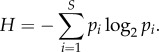
When fission–fusion dynamics occur within the boundaries of a larger, stable group, subgroups can be thought of as subsets of individuals taken from a finite set. Thus, information entropy or information content (hereafter Shannon's entropy; [13]) is an ideal measure for the extent to which subgroup composition is predictable, because the measure was derived precisely for a process in which discrete symbols are selected from a finite set. Suppose that a group of n = 10 individuals can be found divided in subgroups. The total number of different subgroups that can be formed, S, is 2ⁿ − 1 = 1023. If, for instance, all subgroups are equally likely, we would have a 1/1023 chance of guessing the correct composition of a subgroup chosen at random. For such a set of possible subgroup compositions, the information content is equal to log₂(S) ≃ 10 (in bits), which is the average minimal number of yes/no questions needed to figure out the composition of a randomly chosen subgroup. When all the S subgroup compositions are equally likely, the dataset's information content is maximal. More generally, knowing the probability p_i of observing a subgroup with composition i (with i an index ranging from 1 to S), the Shannon's entropy or information content H, for all possible subgroups S with associated probabilities p_i is:

1.1

If all possible subgroup compositions are observed with similar frequencies, H will be near maximal, implying that each observed composition carries a high information content. In contrast, if some subgroup compositions become more likely than others, our uncertainty will decrease (and so will H), i.e. on average, the observation of a particular subgroup composition will reveal less information.

Shannon's entropy is, therefore, directly related to the uncertainty one would have about the composition of a subgroup chosen at random. Thus, we can use the entropy of subgroup composition to compare different species or situations. Moreover, this degree of uncertainty may be a relevant feature not only for the researchers but for the animals themselves. Intuitively, individuals in a group with a high degree of fission–fusion dynamics would face more uncertainty about the composition of the subgroups they can form than individuals of species with less flexible grouping patterns. The more uncertainty in the identity of group-mates, the greater the uncertainty in social interactions [14]. Dealing with such uncertainty is thought to present a cognitive challenge [7,12,15].

We thus propose that Shannon's entropy can be used to quantify social uncertainty due to fission–fusion dynamics at the group and individual levels. At the group level, Shannon's entropy has been used for characterizing the overall degree of variation and uncertainty in social networks [14,16,17]. Accordingly, we propose that the entropy of subgroup composition can be used as a general metric of this particular dimension of fission–fusion dynamics [1]. At the individual level, Shannon's entropy could also reflect the uncertainty actually faced by individuals in these groups. Shannon's entropy has been used to quantify how evenly an individual distributes its grooming interactions among the rest of the individuals in its group [8]. Our proposal is analogous to this use of Shannon's entropy, but applies to the spatiotemporal associations between an individual and the rest of its group mates. When subgroup composition is highly variable, individuals do not repeat their interactions with the same individuals often. A lower frequency of repeated interactions may lead to a higher uncertainty about social relationships, which in turn may require alternate ways of reducing such uncertainty and predicting the outcome of social interactions and others' behaviour [7,14]. Our approach to quantifying this uncertainty should be relevant to any species exhibiting some degree of fission–fusion dynamics, where group members repeat interactions with others, finding themselves associated with others at different frequencies and individually recognizing one another (or at least classifying other group members in broad categories) [1,18].

We develop a proof of concept by measuring Shannon's entropies at the group and individual levels in three species that show different degrees of fission–fusion dynamics: spider monkeys (Ateles geoffroyi), chimpanzees (Pan troglodytes) and gelada monkeys (or geladas, Theropithecus gelada), although our approach should be applicable to any species where the composition of subgroups can be reliably observed and quantified. Although these three primates are known for their high variability in subgroup size and cohesion, they differ in the degree of variation in subgroup composition. Spider monkey and chimpanzee subgroups are highly variable in composition, with group members fissioning and fusing independently from one another [19]. In contrast, geladas have a multi-level social system with highly stable one-male units that fission and fuse with one another in predictable ways, creating a higher order ‘band’ structure [20–22]. Because of this, we predict geladas to have lower entropy values than spider monkeys and chimpanzees, despite the fact that they live in larger groups. We quantify social uncertainty at the group and individual levels using Shannon's entropy and a randomized expectation of entropy that considers subgroup size variation and sample size, against which the observed entropy can be compared. We complement the estimation of social uncertainty with a partition analysis aimed at estimating the number of subgroups that the group is likely to be divided into at any given time, based on the observed composition and size of single focal subgroups.

2. Material and methods

(a). Data collection

Spider monkey data were collected from August 2009 to July 2010 and from January 2013 to September 2014 in the Otoch Ma'ax yetel Kooh protected area, in the Yucatan peninsula, Mexico. The study group has been monitored continuously since 1997, and all group members are identified and habituated to human presence. Observations consisted of instantaneous scan samples performed every 20 min between 06.00 and 18.00 on subgroups chosen according to criteria for homogenizing sample size across individuals. A total of 3916 scan samples, equivalent to 1305 h of observation, were collected in the 2009–2010 period and a total of 7917 scan samples, equivalent to 2639 h of observation, were collected in the 2013–2014 period. During each scan sample, the identities of all subgroup members were recorded. A subgroup was defined using a chain rule of 30 m, such that individuals 30 m or closer to any other were considered as part of the same subgroup [23,24]. Only adult individuals were included in the analysis: 10 females and seven males in 2009–2010 and 18 females and seven males in 2013–2014.

Chimpanzee data were collected from January 2008 to December 2009 from the Sonso community in the Budongo Forest, Uganda. The study group has been monitored continuously since 1990 [25]. All group members are identified and habituated to human presence. Observations consisted of instantaneous scan samples performed every 15 min during focal follows between 06.00 and 18.00, recording the identities of all subgroup members. A subgroup was defined as all individuals visible or known to be present within 35–50 m of the focal animal [25]. Subgroups were chosen each day according to criteria for homogenizing sample size across individuals. The 2008 period contained a total of 10 616 scan samples, equivalent to 2654 h of observation, while the 2009 period contained a total of 12 935 scan samples, equivalent to 3234 h of observation. Only adult individuals that were present throughout each of the entire 2 years were included in the analysis: a total of 20 (in 2008) and 21 (in 2009) females and nine males (both years).

Gelada data were collected from January 2014 to December 2015 in a population that has been continuously monitored since 2006 in the Simien Mountains National Park, Ethiopia [22]. Each morning, observers recorded the identity of all known individuals in a gelada subgroup (defined using a chain rule of 50 m) and then followed it for 1–8 h. During follows, the observers collected a scan sample every 30 min, recording the identity of all known individuals currently in the subgroup. The 2014 period consisted of 1420 scan samples, equivalent to 473 h of observation, and the 2015 period consisted of a total of 1168 scan samples, equivalent to 389 h of observation. Only adult individuals were included in the analysis: 21 males and 82 females in 2014 and 29 males and 97 females in 2015.

(b). Entropy calculation

To quantify social uncertainty at the group level, we calculated Shannon's entropy of subgroup composition as follows. Imagine that a large number of observations allows the accurate estimation of the probability of occurrence of any particular subgroup (or subset) with composition {a}:

2.1

in a group (set) of n elements. The composition entropy H of the group stems from the definition (1.1):

2.2

where the sum runs over all the observed compositions, i.e. those with p_{a}≠0.

To quantify social uncertainty at the individual level, we applied a similar entropy formula, but from the perspective of each individual. For those subgroups in which a given individual i was present, we measured i's entropy by considering the different compositions of the subgroup in terms of the remaining n − 1 individuals (see figure 1).

Figure 1.

Dataset coding for the calculation of subgroup entropy, at group and individual levels. The data consist of observations at regular intervals (rows) on different individuals who can be present (filled circles) or absent (empty circles) in any given subgroup due to fissions and fusions. For calculating the group entropy, we code presences as 1 and absences as 0 and each subgroup composition would correspond to a particular sequence of 1 and 0. For calculating the individual entropy for an individual A, we do the same but only for those subgroups in which A was present and considering all other individuals except A (shaded area), thus capturing the variability in subgroup composition from A's perspective.

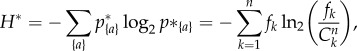
For each entropy, it is useful to determine an upper bound value, denoted as H^*, through a null model neglecting preferential associations: the subsets of size k appear with the same size frequency distribution f_k as in observations, where by normalization, but all the compositions of same size k are assumed to be equiprobable. Given a particular subgroup composition {a} of k_a individuals, there are Cⁿ_ka different ways of choosing k_a elements from n, where Cⁿ_k = n!/[(n − k)!k!] stands for ‘n choose k’. The null conditional probability of {a} given k_a, p*({a}|k_a), takes the form p*({a}|k_a) = 1/Cⁿ_ka. One deduces:

2.3

for the null composition probability p*_{a}. The null maximal entropy follows:

2.4

where, in the last equality, one has used the fact that in the sum over all compositions the terms can be re-arranged by size: each size k as a fixed factor p*_{a} ln ₂p*_{a}, which appears Cⁿ_k times in the sum.

(c). Bootstrap entropy

The number of observations being finite in any empirical dataset, it is often problematic to evaluate the probabilities p_{a} by using equation (2.1), since many compositions of low probability may not be observed and are thus replaced by zero in the sum (2.2). Therefore the empirical H resulting from N_o observations a priori underestimates the real entropy. For a fair comparison of H with a randomized model, it is thus necessary to calculate the entropy of the randomized model given N_o observations as well, instead of equation (2.4). This can be done numerically with a bootstrap or analytically as follows.

Let us denote N(k) = N_of_k as the number of times subgroups of size k have been observed in the data, with . Let us denote n_{a} as the number of times a given composition {a} (of size k_a) is observed from a sampling of size N_o of the null model. The probability that {a} appears exactly i times [i = 0, …, N(k_a)] in this sampling is given by the binomial distribution:

2.5

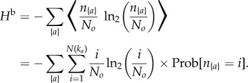
where p*({a}|k_a) = 1/Cⁿ_ka. The bootstrap entropy H^b is obtained by replacing p_{a} by n_{a}/N_o in equation (2.2) and taking the average over all the possible values of n_{a}:

2.6

(The term i = 0 contributes to 0.) Making the substitution as in (2.4) and using equation (2.5), one obtains the bootstrap entropy:

2.7

One recovers equation (2.4) by taking the limit and , keeping N(k)/N₀ = f_k fixed. This entropy is a more useful point of comparison with the observed data because in contrast with the null maximal entropy H^*, where all combinations are equally likely regardless of the sample size, H^b is computed with the sample size of the observed data, the composition of the subgroups being randomized. It is also equal to the mean entropy for a set of bootstrapped original data, in which the 1s and 0s in figure 1 have been randomly shuffled within rows, thus keeping subgroup size and the number of observations for each individual unchanged.

(d). Entropy comparisons

The Kullback–Leibler (KL) divergence is commonly used to quantify how much an empirical distribution p_{a} differs from an expectation p*_{a}, thus providing a way of comparing the observed entropy H to the null maximal entropy H^* [26]. It is defined as and represents, in the present context, the average additional amount of information (in bits) needed to identify a subgroup randomly drawn from p_{a}, when assuming that the distribution is p*_{a}. For the null maximal model, it reads:

2.8

where, once again, k_a represents the size of {a}, p_{a} is given by equation (2.1), and the sum is over all observed compositions.

The above quantity cannot be applied to compare H to the bootstrap entropy H^b, however, since a finite sample of p*_{a} can contain vanishing entries, thus making KL infinite. A useful alternate measure is the Jensen–Shannon (JS) distance between two distributions p and q, defined by , where the entries of m are m_{a} = (p_{a} + q_{a})/2 [26]. Unlike the KL divergence, J can deal with vanishing entries (i.e. {a} such that q_{a} = 0), it is symmetric, and it satisfies the triangle inequality. Another interesting property is that J is 0 if p = q and 1 if the distributions have completely disjoint supports. In other words, if we do not know from which distribution we are choosing a random variable (i.e. if we are choosing from a mixture of p and q), J provides a measure of how much our uncertainty would be reduced by knowing from which distribution, p or q, we are choosing the random variable. This distance is thus adimensional, making comparisons across systems easier a priori. Here, q is a sampling of size N_o of the null model, and we calculate the average of J(p|q), denoted as J^b, over all possible samplings. Following the same steps leading to equation (2.7), the mean distance between observations and the bootstrap reads:

2.9

where the sum runs over observed compositions.

The methods for the partition analysis are included in the electronic supplementary material. All analyses were implemented in R [27] and the code is shared in the electronic supplementary material.

3. Results

(a). Social uncertainty at the group level

The values of entropy (H) at the group level were highly consistent: 8.0–8.5 for spider monkeys, close to 10 for chimpanzees and close to 5 for geladas (figure 2) and significantly lower than the calculated and bootstrap entropies (H^b) in each case. This is confirmed by KL divergences and JS distances (figure 2), which were especially large for geladas.

Figure 2.

(a) Entropy of subgroup composition for two datasets of each of three species: spider monkeys (blue, two upper lines in each graph; data from 2009 and 2013), chimpanzees (green, two middle lines in each graph; data from 2008 and 2009) and geladas (dark red, two lower lines in each graph; data from 2014 and 2015). Solid dots correspond to the observed entropy (H) and empty dots to the bootstrap entropy (H^b). Group size n is 17 and 25 for spider monkeys, 29 and 30 for chimpanzees and 103 and 126 for geladas. Sample size N₀ is 3916 and 7917 for spider monkeys, 10 616 and 12 935 for chimpanzees and 1420 and 1168 for geladas. (b) KL divergence between the observed and the null maximal entropy; (c) JS distance between the observed and the bootstrap entropy, for the same datasets. The observed entropies for spider monkeys and chimpanzees are similar and higher than the geladas'. Also, while the difference between observed and bootstrap entropies is evident in all datasets, it is much larger in geladas than in spider monkeys and chimpanzees.

When considering male-only data for geladas, entropy was relatively unchanged (2014: observed 5.76 bits, bootstrap 10.12 bits; 2015: observed 6.19 bits, bootstrap 10.16 bits) but the KL divergence was lower (2014: KL divergence 9.67; 2015: 16.9; compare to values in figure 2, which are around 70 and 90, for 2014 and 2015, respectively). On the contrary, the JS distance is still close to the maximal value of 1 when considering only the males (2014: 0.95; 2015: 0.99; compare to similar values in figure 2).

(b). Social uncertainty at the individual level

Figure 3 shows summaries of the entropy from the perspective of different individuals. For spider monkeys (figure 3a–b), individual entropy varied from 4 to 8 bits in the case of females and tends to be lower and more consistent in the case of males. While the majority of individuals in 2009 show H values that are clearly lower than the bootstrap entropy H^b values, in 2013 there are several females that show H values that are very close to H^b. When comparing these values using the JS distance (electronic supplementary material, figure S4), there are indeed some females in the 2013 dataset for whom the JS distance between the observed and the bootstrap entropy is relatively low (<0.85), and who could be considered to show a particularly high entropy compared to other females. Their subgroups, thus, seem to show a maximum level of variability in composition.

Figure 3.

Individual entropy of subgroup composition for adult spider monkeys in the 2009 dataset (a) and 2013 dataset (b); chimpanzees in the 2008 dataset (c) and 2009 dataset (d); geladas in the 2014 dataset (e) and 2015 dataset (f). Circles and squares represent females and males, respectively. Solid symbols correspond to the observed entropy (H) and empty symbols to the bootstrap entropy (H^b). Labels for each individual (a–d) or one-male unit or lone male (e–f) in the horizontal axis. While all individuals have a lower observed entropy than the bootstrap, some have a smaller difference, implying that their subgroup composition is close to the maximum, e.g. females AE, AM, ML, PC, SK and TG in (b).

In the case of chimpanzees, we found an opposite effect of sex on the individual entropy values: males tend to have a higher and less variable observed entropy than females (figure 3c–d). The H values for females ranged from 0.88–9.56 bits and those of males ranged from 8.2–9-9 bits. In all individuals, H was clearly lower than H^b in both periods, as can be confirmed by the JS distance values (electronic supplementary material, figure S5). The values of JS distance (electronic supplementary material, figure S5) show more variability amongst individual females than amongst the males.

Gelada individual entropy is aligned to the one-male unit to which individuals belong (figure 3e–f), resulting in females sharing the same individual entropy values as the male. As in the case of the group entropy values (figure 2), individual entropy values were farther from the bootstrap expectation than in the case of the other two species. Comparing these values using the JS distance is not very useful, as most values lie very close to 1 (data not shown). However, limiting the analysis to the one-male units yielded variability in the JS distances, particularly in the 2013 dataset (electronic supplementary material, figure S6). Here, some one-male units have a JS that is farther away from the maximum number, indicating that they have a higher degree of variability in their subgroup compositions.

The results of the partition analysis, aimed at establishing the probability that a group is split into different numbers of subgroups, can be found in the electronic supplementary material.

4. Discussion

We used Shannon's entropy to quantify temporal variation in subgroup composition across three primate species and provide a measure of ‘social uncertainty’ at the group and individual levels. As predicted, spider monkeys and chimpanzees, considered as species with a high degree of fission–fusion dynamics [1,19], have a higher entropy of subgroup composition than geladas, which show variation in subgroup size and spatial cohesion between group members, but also have indivisible one-male units and a higher order band structure [20]. This latter characteristic constrains the flexibility in subgroup composition of geladas compared to spider monkeys and chimpanzees, and explains why geladas have a lower observed entropy.

That variation in sample size and group size within a species does not influence the estimation of entropy suggests that our method is robust and could be used to compare social uncertainty across different species and datasets with different characteristics. The bootstrap entropy H^b, corresponding to the maximum entropy that could be expected in a dataset of the same size and subgroup size distribution if all subgroup compositions were equally likely, serves as a reference to evaluate whether the observed entropy is relatively high or low. In all three species, that the observed entropy is lower than the bootstrap entropy implies that preferential associations between individuals make some compositions more likely than others among the full set of potential compositions. Together, the observed and bootstrap entropies serve as a measure of how much of the potential variation in subgroup composition is actually observed.

We propose that our method can be used to compare the degree of fission–fusion dynamics between species, particularly in terms of the temporal variation in subgroup composition. In particular, JS distances serve as a quantification of how far the observed entropy is from the bootstrap entropy and can be used as for comparative purposes. A species with a high JS distance (close to unity) would have a variation in subgroup composition that is far from the maximum expected by the bootstrap entropy and would have a relatively low degree of temporal variation in subgroup composition. Conversely, a species with a low JS distance would have a variation in subgroup composition that is close to the maximum expected and thus would have a relatively high degree of temporal variation in this dimension of fission–fusion dynamics. In our analysis, geladas stood out as having the highest JS distance relative to the bootstrap entropy and thus would be the species with the lowest degree of variation in subgroup composition. The implication is that there are more constraints to the flexibility of association, and thus a lower uncertainty in subgroup composition, in geladas than in the other two species. The difference in JS distances between spider monkeys and chimpanzees, although not as high as between these two species and the geladas, is still detectable and suggests that chimpanzees have the highest degree of temporal variation in this dimension of fission–fusion dynamics of the three analysed species. JS distances can also be used to explore within-species differences in the temporal variation in subgroup composition. As figure 2 shows, for spider monkeys JS distance is larger in 2009 than in 2013, whereas JS distances of the two chimpanzee datasets are rather similar.

The level of analysis of social uncertainty for geladas deserves special attention. The existence of indivisible, one-male units decreases the number of potential subgroup compositions and thus the observed entropy when considering all individuals. We also ran the analysis considering only males, thus estimating the degree of flexibility of association between one-male units. We obtained similar values of entropy at both levels, with an observed entropy around 4 bits lower than the bootstrap expectation. This result is what would be expected if one-male units associated preferentially with a few of the other one-male units, as opposed to associating freely with all units. In other words, a low value of entropy in the association of one-male units into bands (i.e. the clearest, more consistently observed level above the one-male units; [22]) implies that the composition of these bands is relatively predictable. The JS distances between observed and bootstrap entropies when considering only males were close to 1, suggesting that there is much less variation than could be expected if there were no preferential associations between one-male units. However, the fact that there are many more males in 2014 apparently leads to much more predictable patterns (i.e. JS distances close to unity in all cases). It is as if the one-male units responded by becoming less fluid, perhaps as a way of maintaining a low uncertainty in the face of an increase in group size and all the potential disorder (i.e. higher entropy) this could cause. The non-random association of one-male units in this population of geladas has been demonstrated using both social network analysis [21] and hierarchical clustering [22]. Thus, our results are consistent with what we know about gelada multilevel society, but they go a step further by quantifying a component of social complexity that is closely related to social uncertainty due to fission–fusion dynamics and that can be compared between and within species.

We also extended our analysis to the entropy of subgroup composition from the point of view of each group member. Overall, we obtained values similar to those for the whole group, but some differences between individual values of entropy were revealing. In spider monkeys and chimpanzees, the two sexes differed in their individual entropy values. Higher values in female spider monkeys compared to males are consistent with the females' lower rates of preferential association compared to males [28]. By contrast, lower values in female chimpanzees compared to males could be due to their known tendency to form strong and lasting bonds with particular females [29], as well as to the opportunistic nature of associations between males [30]. In spider monkeys, the females with a lowest JS distance had recently immigrated into the group (i.e. females AE, HI, PC and TG in electronic supplementary material, figure S4b). This result is consistent with previous studies [28] that found that during their first year in the group, immigrant females' preference for specific individuals is low. This is an example of the utility of comparing the observed and bootstrap entropy values using the JS distance. In the case of chimpanzees, the 2009 data contained a newly immigrating female (TJ), which also had a relatively low JS distance value compared to other individuals (electronic supplementary material, figure 5Sb). Other females with particularly high JS distances include BC, KG and FL, who had severe snare injuries (entire hand or foot missing), and thus limited their movements to the core area of the home range and were observed in smaller subgroups than the rest of the females. This is an example of the usefulness of comparing observed entropy values between individuals.

An individual's entropy value can be interpreted as the degree of uncertainty it has about its particular set of associations, with higher entropy values indicating higher uncertainty [14]. It has long been established that several social interactions are aimed at reducing the stress caused by uncertainty in social relationships [31,32]. A reduction in uncertainty has been proposed to lie at the core of emerging features of social structure such as dominance hierarchies [14,33,34]. In species where repeated social interactions occur among group members that form subgroups, our measures of entropy at the individual level are a promising metric for quantifying social uncertainty due to fission–fusion dynamics and for comparing this component of social complexity across individuals, situations, groups, and species. Individuals with a lower observed entropy relative to the bootstrap entropy would face less uncertainty than individuals with similar values of observed and bootstrap entropy. Analysing these individual differences may help researchers understand the role played by individuals in their groups and the extent to which they could predict the interactions amongst others in the group [35].

One of the reasons a high degree of fission–fusion dynamics is considered to be cognitively challenging is that individuals face a high uncertainty about their social relationships [1]. For social interactions to reduce the uncertainty about other group member's behaviour and the quality of relationships with them [31], specific mechanisms must be in place that can allow individuals to update their information about these relationships with others, as well as to generalize across different relationships that share similar features. Therefore, cognitive abilities that allow individuals to reduce their uncertainty with respect to social relationships, like abstraction (e.g. using concepts such as ‘friend’ or ‘potential mate’ to classify relationships) and transitivity (i.e. inferring a linear order of relationships using partial information), may be particularly important in species with high levels of fission–fusion dynamics, where the understanding of social relationships must be carried out using partial information in highly variable social contexts [6]. In addition, cognitive abilities to deal with uncertainty, such as inhibition of ongoing responses until the social situation can be assessed when subgroup composition changes, are also important in fission–fusion dynamics [36]. We predict that species with a high uncertainty in subgroup composition are more likely to show these cognitive abilities than species with a lower uncertainty.

Estimating the probability that the whole group would be partitioned, or split, in different numbers of subgroups provides a further way to quantify social uncertainty. The probability distributions that result from our partition analysis can be considered as a measure of the uncertainty with respect to the grouping patterns of unobserved group members. For example, it might be easier for an individual to predict which group members not present in its current subgroup could be close or associated with one another in a group that is potentially split in 2-6 subgroups than in a group that is split in 9-14 subgroups (e.g. compare electronic supplementary material, figure S9a and b). In addition to its usefulness for studying higher levels in multi-level societies, our partition analysis could be more generally applied in any study in which only one subgroup can be followed at one time (like in the majority of studies of species with a high degree of fission–fusion dynamics). For example, research on topics like between-subgroup vocal interactions [23,37] or home ranges [38,39] could be aided by an estimation of how many subgroups there are likely to be at a given time, even if only one subgroup has been monitored directly.

It is necessary to note that our method assumes that the distribution of observed subgroup size f_k reflects the true distribution of subgroup size in which a group was found during a certain study period. Under that assumption, the bootstrap entropy H^b reflects the maximum entropy that could be observed given the observed distribution of subgroup size. Also, our estimation of the most likely partition in which the group is found relies on a correctly estimated f_k. However, when studying species with high degrees of fission–fusion dynamics, there are potential biases which might make it more likely for researchers to observe the larger or more conspicuous subgroups. Thus, in field studies, steps should be taken to ensure that the sample of subgroups is representative of the true distribution.

Establishing metrics to estimate social complexity is not a trivial matter [12,40,41]. Crude measures, such as group size, number of different interactions, presence of triadic interactions, etc., have been used but have not been operationalized in such a way that different species with different group size and degree of fission–fusion dynamics can be compared (but see [10]). As we show, Shannon's entropy represents a relevant metric of social uncertainty as one component of social complexity, but it is important to bear in mind the relationship between complexity and uncertainty. While a completely random process, which in turn would have the highest entropy, would be maximally uncertain, we would not necessarily consider it as a complex process. On the opposite end, a fully predictable pattern, with minimal complexity, would also be minimally uncertain, with a correspondingly low entropy. When considering complexity, including social complexity, we need to take into account both the flexibility and the nonrandom structure of a process [42, p. 353],[43]. Thus, maximally complex societies would not necessarily lie in any of the two extremes of the uncertainty spectrum. A middle-ground, where relationships are somewhat predictable, also corresponds to the greatest degree of relationship differentiation, which is another way to characterize social complexity [10]. This is because random processes would involve no relationship differentiation, while completely stable groups can emerge from simple rules that involve only a categorical differentiation between in and out-group individuals. We predict that, in terms of subgroup composition, higher social complexity would occur in groups with high observed entropy that is, nonetheless, still lower than the bootstrap entropy. In terms of JS distances, a species would have a higher social complexity at intermediate values. In these groups, individuals would have to cope with a high degree of uncertainty about who their associates would be at any one time but at the same time maintain a diversity of social relationships with preferred companions in many different contexts [10,11,32,34]. It is possible that the real complexity might lie in the cognitive and behavioural mechanisms used to deal with social uncertainty in the face of an existing social structure.

Our approach to measuring social complexity through social uncertainty can be applied to any species that interacts in temporary and variable subsets and may be particularly relevant for taxa in which a known set of individuals can recognize one another through visual, vocal, or olfactory means. The proposed metrics should also be useful for future studies comparing the degree of fission–fusion dynamics across species varying to different extents in subgroup composition, together with subgroup size and spatial cohesion [1]. More generally, they can aid our understanding of the influence of flexible social settings on the interactions between group members and their implications for social cognition.

Ethics

All fieldwork was conducted under the Guidelines for the Use of Animals in Research of the Association for the Study of Animal Behaviour/Animal Behavior Society and conformed to the legal requirements of the respective countries where it was conducted.

Data accessibility

All datasets used to illustrate the methodology are shared in a data repository. We also share the code in R [27] to calculate the entropy measures, both at the group and individual levels, the comparison of entropies using the KL divergences and the JS distances, as well as the partition analysis (see electronic supplementary material).

Authors' contributions

The study was conceived by G.R.F., A.J.K., F.A. and D.B. The study was designed by G.R.F., A.J.K., M.C.C., A.D., J.L., C.M.S., F.A. and D.B. Field data were collated by J.L., J.C.B., T.C.B., N.S.M. and K.S. Data analysis was carried out by G.R.F. and D.B., with techniques developed by D.B. The workshop where ideas were first discussed was coordinated by F.A. and C.M.S. The manuscript was drafted by all coauthors, who also gave final approval for publication.

Competing interests

We declare we have no competing interests.

Funding

This study was first discussed at a Workshop on Fission–Fusion Dynamics funded by the Wenner-Gren Foundation (F.A. and C.M.S.). Funding was provided by CONACYT and Instituto Politécnico Nacional (G.R.F.), Santander Mobility Award/Swansea University (A.J.K.), Wildlife Conservation Society, National Geographic Society, Leakey Foundation, National Science Foundation and the National Institute on Aging (T.J.B., J.C.B. and N.S.M.), National Geographic, CONACYT and Chester Zoo (F.A. and C.S.), UNAM PAPIIT-105015 (D.B.), NSF IOS-1255974, BCS-0715179 (T.B. and J.B.), SBE-1723237 and NIH R00-AG051764 (N.S.M.) (T.B. and J.B.) and NSF III 1514174 and David and Lucile Packard Foundation 2016-65130 (M.C.C.).

References

- 1.Aureli F. et al. 2008. Fission–fusion dynamics: new research frameworks. Curr. Anthropol. 49, 627–654. ( 10.1086/586708) [DOI] [Google Scholar]
- 2.Kummer H. 1971. Primate societies: group techniques of ecological adaptation. Chicago, IL: Aldine-Atherton. [Google Scholar]
- 3.Chapman CA, Chapman LJ, Wrangham R. 1995. Ecological constraints on group size: an analysis of spider monkey and chimpanzee subgroups. Behav. Ecol. Sociobiol. 36, 59–70. ( 10.1007/BF00175729) [DOI] [Google Scholar]
- 4.Smith JE, Kolowski JM, Graham KE, Dawes SE, Holekamp KE. 2008. Social and ecological determinants of fission–fusion dynamics in the spotted hyaena. Anim. Behav. 76, 619–636. ( 10.1016/j.anbehav.2008.05.001) [DOI] [Google Scholar]
- 5.Asensio N, Korstjens AH, Aureli F. 2009. Fissioning minimizes ranging costs in spider monkeys: a multiple-level approach. Behav. Ecol. Sociobiol. 63, 649–659. ( 10.1007/s00265-008-0699-9) [DOI] [Google Scholar]
- 6.Cheney DL, Seyfarth RM. 1990. How monkeys see the world: inside the mind of another species. Chicago, IL: Chicago University Press. [Google Scholar]
- 7.Bergman TJ, Sheehan MJ. 2013. Social knowledge and signals in primates. Am. J. Primatol. 75, 683–694. ( 10.1002/ajp.22103) [DOI] [PubMed] [Google Scholar]
- 8.Cheney DL. 1992. Intragroup cohesion and intergroup hostility: the relation between grooming distributions and intergroup competition among female primates. Behav. Ecol. 3, 334–345. ( 10.1093/beheco/3.4.334) [DOI] [Google Scholar]
- 9.Di Bitetti MS. 2000. The distribution of grooming among female primates: testing hypotheses with the Shannon–Wiener diversity index. Behaviour 137, 1517–1540. ( 10.1163/156853900502709) [DOI] [Google Scholar]
- 10.Fischer J, Farnworth MS, Sennhenn-Reulen H, Hammerschmidt K. 2017. Quantifying social complexity. Anim. Behav. 130, 57–66. ( 10.1016/j.anbehav.2017.06.003) [DOI] [Google Scholar]
- 11.Freeberg TM, Dunbar RI, Ord TJ. 2012. Social complexity as a proximate and ultimate factor in communicative complexity. Phil. Trans. R. Soc. B 367, 1785–1801. ( 10.1098/rstb.2011.0213) [DOI] [PMC free article] [PubMed] [Google Scholar]
- 12.Bergman TJ, Beehner JC. 2015. Measuring social complexity. Anim. Behav. 103, 203–209. ( 10.1016/j.anbehav.2015.02.018) [DOI] [Google Scholar]
- 13.Shannon C. 1948. A mathematical theory of communication. Bell Syst. Tech. J. 27, 379–423. ( 10.1002/j.1538-7305.1948.tb01338.x) [DOI] [Google Scholar]
- 14.Barrett L, Henzi SP, Lusseau D. 2012. Taking sociality seriously: the structure of multi-dimensional social networks as a source of information for individuals. Phil. Trans. R. Soc. B 367, 2108–2118. ( 10.1098/rstb.2012.0113) [DOI] [PMC free article] [PubMed] [Google Scholar]
- 15.Dunbar RI, Shultz S. 2010. Bondedness and sociality. Behaviour 147, 775–803. ( 10.1163/000579510X501151) [DOI] [Google Scholar]
- 16.Bailey KD. 1990. Social entropy theory. Albany, NY: SUNY Press. [Google Scholar]
- 17.Haddadi H, King AJ, Wills AP, Fay D, Lowe J, Morton AJ, Hailes S, Wilson AM. 2011. Determining association networks in social animals: choosing spatial temporal criteria and sampling rates. Behav. Ecol. Sociobiol. 65, 1659–1668. ( 10.1007/s00265-011-1193-3) [DOI] [Google Scholar]
- 18.Loretto MC, Schuster R, Itty C, Marchand P, Genero F, Bugnyar T. 2017. Fission–fusion dynamics over large distances in raven non-breeders. Sci. Rep. 7, 380 ( 10.1038/s41598-017-00404-4) [DOI] [PMC free article] [PubMed] [Google Scholar]
- 19.Symington MM. 1990. Fission–fusion social organization in Ateles and Pan. Int. J. Primatol. 11, 47–61. ( 10.1007/BF02193695) [DOI] [Google Scholar]
- 20.Dunbar R. 1975. Social dynamics of gelada baboons. Basel, Switzerland: Karger. [PubMed] [Google Scholar]
- 21.Mac Carron P, Dunbar R. 2016. Identifying natural grouping structure in gelada baboons: a network approach. Anim. Behav. 114, 119–128. ( 10.1016/j.anbehav.2016.01.026) [DOI] [Google Scholar]
- 22.Snyder-Mackler N, Beehner JC, Bergman TJ. 2012. Defining higher levels in the multilevel societies of geladas (Theropithecus gelada). Int. J. Primatol. 33, 1054–1068. ( 10.1007/s10764-012-9584-5) [DOI] [Google Scholar]
- 23.Ramos-Fernández G. 2005. Vocal communication in a fission–fusion society: do spider monkeys stay in touch with close associates? Int. J. Primatol. 26, 1077–1092. ( 10.1007/s10764-005-6459-z) [DOI] [Google Scholar]
- 24.Aureli F, Schaffner CM, Asensio N, Lusseau D. 2012. What is a subgroup? How socioecological factors influence interindividual distance. Behav. Ecol. 23, 1308–1315. ( 10.1093/beheco/ars122) [DOI] [Google Scholar]
- 25.Reynolds V. 2005. The chimpanzees of the Budongo forest: ecology, behaviour and conservation. Oxford, UK: Oxford University Press. [Google Scholar]
- 26.Lin J. 1991. Divergence measures based on the Shannon entropy. IEEE Trans. Inf. Theory 37, 145–151. ( 10.1109/18.61115) [DOI] [Google Scholar]
- 27.R Core Team. 2016. R: a language and environment for statistical computing. Vienna, Austria: R Foundation for Statistical Computing. [Google Scholar]
- 28.Ramos-Fernandez G, Boyer D, Aureli F, Vick LG. 2009. Association networks in spider monkeys (Ateles geoffroyi). Behav. Ecol. Sociobiol. 63, 999–1013. ( 10.1007/s00265-009-0719-4) [DOI] [Google Scholar]
- 29.Foerster S, McLellan K, Schroepfer-Walker K, Murray CM, Krupenye C, Gilby IC, Pusey AE. 2015. Social bonds in the dispersing sex: partner preferences among adult female chimpanzees. Anim. Behav. 105, 139–152. ( 10.1016/j.anbehav.2015.04.012) [DOI] [PMC free article] [PubMed] [Google Scholar]
- 30.Gilby IC, Wrangham RW. 2008. Association patterns among wild chimpanzees (Pan troglodytes schweinfurthii) reflect sex differences in cooperation. Behav. Ecol. Sociobiol. 62, 1831 ( 10.1007/s00265-008-0612-6) [DOI] [Google Scholar]
- 31.Van Hooff JARAM, Aureli F. 1994. Social homeostasis and the regulation of emotion. In Emotions: essays on emotion theory, pp. 197–217 (eds van Goozen HM, de Poll NE, Segeant JA). Hillsdale, NJ: Lawrence Erlbaum Associates, Inc., Publishers. [Google Scholar]
- 32.Wittig RM, Crockford C, Lehmann J, Whitten PL, Seyfarth RM, Cheney DL. 2008. Focused grooming networks and stress alleviation in wild female baboons. Horm. Behav. 54, 170–177. ( 10.1016/j.yhbeh.2008.02.009) [DOI] [PMC free article] [PubMed] [Google Scholar]
- 33.Drews C. 1993. The concept and definition of dominance in animal behaviour. Behaviour 125, 283–313. ( 10.1163/156853993X00290) [DOI] [Google Scholar]
- 34.Flack JC. 2012. Multiple time-scales and the developmental dynamics of social systems. Phil. Trans. R. Soc. B 367, 1802–1810. ( 10.1098/rstb.2011.0214) [DOI] [PMC free article] [PubMed] [Google Scholar]
- 35.Flack J. 2017. 12 Life's information hierarchy. In From matter to life: information and causality (eds Walker SI, Davies PCW, Ellis GFR), pp. 283–302. Cambridge, UK: Cambridge University Press. [Google Scholar]
- 36.Amici F, Aureli F, Call J. 2008. Fission–fusion dynamics, behavioral flexibility, and inhibitory control in primates. Curr. Biol. 18, 1415–1419. ( 10.1016/j.cub.2008.08.020) [DOI] [PubMed] [Google Scholar]
- 37.Cantor M, Shoemaker LG, Cabral RB, Flores CO, Varga M, Whitehead H. 2015. Multilevel animal societies can emerge from cultural transmission. Nat. Commun. 6, 8091 ( 10.1038/ncomms9091) [DOI] [PMC free article] [PubMed] [Google Scholar]
- 38.Smith-Aguilar SE, Ramos-Fernández G, Getz WM. 2016. Seasonal changes in socio-spatial structure in a group of free-living spider monkeys (Ateles geoffroyi). PLoS ONE 11, e0157228 ( 10.1371/journal.pone.0157228) [DOI] [PMC free article] [PubMed] [Google Scholar]
- 39.Sprogis KR, Raudino HC, Rankin R, MacLeod CD, Bejder L. 2016. Home range size of adult Indo-Pacific bottlenose dolphins (Tursiops aduncus) in a coastal and estuarine system is habitat and sex-specific. Mar. Mammal Sci. 32, 287–308. ( 10.1111/mms.12260) [DOI] [Google Scholar]
- 40.Whiten A. 2000. Social complexity and social intelligence. Nat. Intell. 233, 185–196. [DOI] [PubMed] [Google Scholar]
- 41.Whitehead H. 2008. Analyzing animal societies: quantitative methods for vertebrate social analysis. Chicago, IL: University of Chicago Press. [Google Scholar]
- 42.Gleick J. 2012. The information: a history, a theory, a flood. New York, NY: Vintage Books. [Google Scholar]
- 43.Prokopenko M, Boschetti F, Ryan AJ. 2008. An information-theoretic primer on complexity, self-organization, and emergence. Complexity 15, 11–28. ( 10.1002/cplx.20249) [DOI] [Google Scholar]
Associated Data
This section collects any data citations, data availability statements, or supplementary materials included in this article.
Supplementary Materials
Data Availability Statement