Convolutional Neural Network based Metal Artifact Reduction in X-ray Computed Tomography

Abstract

In the presence of metal implants, metal artifacts are introduced to x-ray CT images. Although a large number of metal artifact reduction (MAR) methods have been proposed in the past decades, MAR is still one of the major problems in clinical x-ray CT. In this work, we develop a convolutional neural network (CNN) based open MAR framework, which fuses the information from the original and corrected images to suppress artifacts. The proposed approach consists two phases. In the CNN training phase, we build a database consisting of metal-free, metal-inserted and pre-corrected CT images, and image patches are extracted and used for CNN training. In the MAR phase, the uncorrected and pre-corrected images are used as the input of the trained CNN to generate a CNN image with reduced artifacts. To further reduce the remaining artifacts, water equivalent tissues in a CNN image are set to a uniform value to yield a CNN prior, whose forward projections are used to replace the metal-affected projections, followed by the FBP reconstruction. The effectiveness of the proposed method is validated on both simulated and real data. Experimental results demonstrate the superior MAR capability of the proposed method to its competitors in terms of artifact suppression and preservation of anatomical structures in the vicinity of metal implants.

I. Introduction

Patients are usually implanted with metals, such as dental fillings, hip prostheses, coiling, etc. These highly attenuated metallic implants lead to severe beam hardening, photon starvation, scatter, and so on. This brings strong star-shape or streak artifacts to the reconstructed CT images [1]. Although a large number of metal artifact reduction (MAR) methods have been proposed during the past four decades, there is still no standard solution [2]–[4]. Currently, how to reduce metal artifacts remains a challenging problem in the x-ray CT imaging field.

Metal artifact reduction algorithms can be generally classified into three groups: physical effects correction, interpolation in projection domain and iterative reconstruction. A direct way to reduce artifacts is to correct physical effects, e.g., beam hardening [5]–[7] and photon starvation [8]. However, in the presence of high-atom number metals, errors are so strong that the aforementioned corrections cannot achieve satisfactory results. Hence, the metal-affected projections are assumed as missing and replaced with surrogates [9]–[11]. Linear interpolation (LI) is a widely used MAR method, where the missing data is approximated by the linear interpolation of its neighboring unaffected projections for each projection view. The LI usually introduces new artifacts and distorts structures near large metals [12]. By comparison, by employing a priori information, the forward projection of a prior image is usually a more accurate surrogate for the missing data [13]–[17]. The normalized MAR (NMAR) is a state-of-the-art prior image based MAR method, which applies a thresholding based tissue classification on the uncorrected image or the LI corrected image to remove most of the artifacts and produce a prior image [14]. In some cases, artifacts are so strong that some image pixels are classified into wrong tissue types, leading to inaccurate prior images and unsatisfactory results. The last group of methods iteratively reconstruct images from the unaffected projections [18]–[21] or weighted/corrected projections [22]. With proper regularizations, the artifacts are suppressed in the reconstructed results. However, due to the high complexity of various metal materials, sizes, positions, and so on, it is hard to achieve satisfactory results for all cases using a single MAR strategy. Therefore, several researchers combined two or three types of MAR techniques as hybrid methods [23] [24], fusing the merits of various MAR techniques. Hence, the hybrid strategy has a great potential to obtain more robust and outstanding performance by appropriately compromising a variety of MAR approaches.

Recently, deep learning has achieved great successes in the image processing and pattern recognition field. For example, the convolutional neural network (CNN) has been applied to medical imaging for low dose CT reconstruction and artifacts reduction [25]–[34]. In particular, the concept of deep learning was introduced to metal artifact reduction for the first time in 2017 [29], [31], [35]–[39]. Park et al. employed a U-Net to correct metal-induced beam hardening in the projection domain [38] and image domain [39], respectively. Their simulation studies showed promising results over hip prostheses of titanium. However, the beam hardening correction based MAR methods have limited capability for artifact reduction in the presence of high-Z metal. Gjesteby et al. developed a few deep learning based MAR methods that refine the performance of the state-of-the-art MAR method, NMAR, with deep learning in the projection domain [29] and image domain [31], [35], respectively. The CNN was used to help overcome residual errors from the NMAR. While their experiments demonstrated that CNN can improve the NMAR effectively, remaining artifacts are still considerable. Simultaneously, based on the CNN, we proposed a general open framework for MAR [36], [37]. This paper is a comprehensive extension of our previous work [36]. We adopt the CNN as an information fusion tool to produce a reduced-artifact image from some other methods corrected images. Specifically, before the MAR, we build a MAR database to generate training data for the CNN. For each clinical metal-free patient image, we simulate the metal artifacts and then obtain the corresponding corrected images by several representative MAR methods. Without loss of generality, we apply a beam hardening correction (BHC) method and the linear interpolation (LI) method in this study. Then, we train a CNN for MAR. The uncorrected, BHC and LI corrected images are stacked as a three-channel image, which is the input data of CNN and the corresponding metal-free image is the target, and a metal artifact reduction CNN is trained. In the MAR phase, the pre-corrected images are obtained using the BHC and LI methods, and these two images and the uncorrected image are put into the trained CNN to obtain the corrected CNN image. To further reduce the remaining artifacts, we incorporate the strategy of prior image based methods. Specifically, a tissue processing step is introduced to generate a prior from the CNN image, and the forward projection of the prior image is used to replace metal-affected projections. The advantages of the proposed method are threefold. First, we combine the corrected results from various MAR methods as the training data. In the end-to-end CNN training, the information from different correction methods is captured and the merits of these methods are fused, leading to a higher quality image. Second, the proposed method is an open framework, and all the MAR methods can be incorporated into this framework. Third, this method is data driven. It has a great potential to improve the CNN capability if we continue increasing the training data with more MAR methods. The source codes of our proposed method are open¹.

The rest of the paper is organized as follows. Section II describes the creation of metal artifact database and the training of a convolutional neural network. Section III develops the CNN based MAR method. Section IV describes the experimental settings. Section V gives the experimental results and analyzes properties of the proposed method. Finally, Section VI discusses some relevant issues and concludes the paper.

II. Training of the Convolutional Neural Network

There are two phases to train a convolutional neural network for MAR. First, we generate metal-free, metal-inserted and MAR corrected CT images to create a database. Then, a CNN is constructed and the training data is collected from the established database and used to train the CNN.

A. Establishing a Metal Artifact Database

At first, we need to create a CT image database for CNN training. In this database, for each case, metal-free, metal-inserted, and MAR methods processed images are included.

1) Generating Metal-free and Metal-inserted Images

In this subsection, we describe how to generate metal-free and metal-inserted CT images, where beam hardening and Poisson noise are simulated. To ensure that the trained CNN works for real cases, instead of using phantoms, we simulate the metal artifacts based on clinical CT images. To begin with, a number of DICOM format clinical CT images are collected from online resources and “the 2016 Low-dose CT Grand Challenge” training dataset [40]. In the presence of metal implants, we manually segment metals and store them as small binary images, which represent typical metallic shapes in real cases. Several representative metal-free CT images are selected as benchmark images. For a given benchmark image, its pixel values are converted from CT values to linear attenuation coefficients and denoted as x. To simulate polychromatic projection, we need to know the material components in each pixel. Hence, a soft threshold-based weighting method [41] is applied to segment the image x into bone and water-equivalent tissue components, denoted as x^b and x^w, respectively. Pixels with values below a certain threshold T₁ are viewed as water equivalent, while pixels above a higher threshold T₂ are assumed to be bone. The pixels with values between T₁ and T₂ are assumed to be a mixture of water and bone. Thus, a weighting function for bone is introduced as

$$\omega (x_i)=\{\begin{array}{ll}0,\hfill & x_i\le T_2\hfill \\ 1,\hfill & x_i\ge T_2\hfill \\ \frac{x_i-T_1}{T_2-T_1}\hfill & T_1<x_i<T_2\hfill \end{array},$$ (1)

where x is the i^th pixel value of x. Hence, x^b and x^w are expressed as

$$x_i^b=\omega (x_i)x_i,$$ (2)

$$x_i^w=(1-\omega (x_i))x_i.$$ (3)

Fig. 1 gives an example of the image segmentation.

Fig. 1.

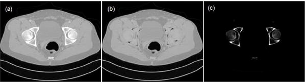
Example of tissue segmentation. (a) The benchmark image, (b) water-equivalent tissue and (c) bone.

For an x-ray path L_j, the linear integral of water and bone images are $d_j^w$ and $d_j^b$, respectively. We have

$$d_j^k={\displaystyle {\int }_{L_j}{\mathrm{x}}^{k}dl},$$ (4)

where the superscript “k” indicates “w” or “b”. To simulate polychromatic projections, we need to obtain linear attenuation maps of water and bone at various energies. For each material, the linear attenuation coefficient at the pixel is the product of the known energy-dependent mass attenuation coefficient and the unknown energy-independent density [42]. We have

$$x_i^k(E)=m^k(E){\rho }_i^k,$$ (5)

where ${\rho }_i^k$ is the density of “k” material at the i^th pixel, and m^w(E) and m^b(E) are respectively mass attenuation coefficients at energy E of water and bone. For a given polychromatic x-ray imaging system, let us assume that the equivalent monochromatic energy is E₀. Then, $x_i^b$ and $x_i^w$ can be written as

$$x_i^k=x_i^k(E_0)=m^k(E_0){\rho }_i^k.$$ (6)

Combining Eqs. (5) and (6), the unknown density ${\rho }_i^k$ can be eliminated. Hence, the energy dependent linear attenuation coefficient for each material is obtained as the following,

$$x_i^k(E)=\frac{x_i^k{m}^k(E)}{m^k(E_0)}.$$ (7)

for the given x-ray path L_j, the ideal projection measurement ${\overline{y}}_j$ recorded by the j^th detector bin is

$$\begin{gathered} {\overline{y}}_j={\displaystyle \int I(E)\exp }\left(-{\displaystyle {\int }_{L_j}\left(x_i^w(E)+x_i^b(E)\right)dl}\right)dE \\ ={\displaystyle \int I(E)\exp }\left(-{\displaystyle {\int }_{L_j}\left(\frac{x_i^w{m}^w(E)}{m^w(E_0)}+\frac{x_i^b{m}^b(E)}{m^b(E_0)}\right)}dl\right)dE, \\ ={\displaystyle \int I(E)\exp }\left(-\frac{m^w(E)d_j^w}{m^w(E_0)}-\frac{m^b(E)d_j^b}{m^b(E_0)}\right)dE \end{gathered}$$ (8)

where I(E) is the known energy dependence of both the incident x-ray source spectrum and the detector sensitivity. Because the linear projection d^w and $d_j^b$ have been computed in advance, computing the polychromatic projection using Eq. (8) is very efficient. Approximately, the measured data follow the Poisson distribution:

$$y_j~\text{Poisson}\{{\overline{y}}_j+r_j\},$$ (9)

where r_j is the mean number of background events and readout noise variance, which is assumed as a known nonnegative constant [42], [43]. Thus, the noisy polychromatic projection p for reconstruction can be expressed as:

$p_j=-\ln \frac{y_i}{{\displaystyle \int I(E)dE}},$ (10)

The metal-free image is reconstructed using filtered backprojection (FBP), and the image is assumed as reference and denoted as x^ref.

To simulate metal artifacts, one or more binary metal shapes are placed into proper anatomical positions, generating a metal-only image x^m. We specify the metal material, and assign metal pixels with linear attenuation coefficient of this material at energy E₀, and set the rest pixels to be zero. Because metals are inserted into patients, pixel values in x^b and x^w are set to be zero if the corresponding pixels in x^m are nonzero. Then, the $d_j^w$ and $d_j^b$ are updated, and the corresponding metal projection is computed using Eq. (4). Similar to Eq. (8), the ideal projection measurement is

$${\overline{y}}_j^{\ast }={\displaystyle \int I(E)\exp }\left(-\frac{m^w(E)d_j^w}{m^w(E_0)}-\frac{m^b(E)d_j^b}{m^b(E_0)}-\frac{m^m(E)d_j^m}{m^m(E_0)}\right)dE,$$ (11)

where m^m(E) is the mass attenuation coefficient of the metal at energy E. Following the same operations in Eqs. (9) and (10), the noisy polychromatic projection p* is obtained, and then the image x^art containing artifacts is reconstructed. Fig. 2 shows four samples in the database. The top four rows in Fig. 2 are benchmark images, metal-only images, metal-free images and metal-inserted images, respectively.

Fig. 2.

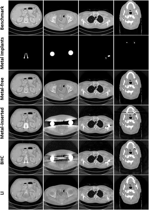
Representative samples in the database. Each column corresponds to one case. The top four rows are benchmark images, metal-only images, metal-free and metal-inserted images, respectively. The last two rows are images after metal artifact reduction using the BHC and LI, respectively.

2) Simple Metal Artifact Reduction

We apply two simple metal artifact reduction methods, the linear interpolation (LI) and beam hardening correction (BHC) [44], to alleviate artifacts. These methods are fast and easy to implement, and there are no manually selected parameters. Moreover, they suppress metal artifacts with different schemes, which have a great potential to provide complementary information for the CNN. In the LI method, the metal-affected projections are identified and replaced with the linear interpolation of their unaffected neighboring projections in each projection view. The LI corrected image is denoted as x^LI. The BHC approach [44] adopts a first-order model of beam hardening error to compensate for the metal-affected projections. The length of metal $\left\{l_j^m\right\}$ along each x-ray path is computed by forward projecting the binary metal-only image. The difference $\left\{p_j^m\right\}$ between the original and LI projections is assumed as the contribution of metal. The correction curve between $\left\{l_j^m\right\}$ and $\left\{p_j^m\right\}$ is fitted to the correlation using a least squares cubic spline fit. Finally, the correction curve is subtracted from the original projection to yield the corrected data. The image obtained using BHC is denoted as x^BHC. The two bottom rows in Fig. 2 are four samples of BHC and LI corrected images, where metals are not inserted back into the LI images.

B. Training a Convolutional Neural Network (CNN)

For each sample in the database, the original uncorrected image, BHC image and LI image are combined as a three-channel image. The samples in the database are randomly divided into two groups for CNN training and validation. Small image patches of s × t × 3 are extracted from three-channel images, and these patches are assumed as the input data of CNN. Correspondingly, image patches of s × t are also obtained from the same positions of the metal-free images, and these patches are assumed as the target of CNN during training. The r^th training sample pair is denoted as u ∈ ℝ^s×t×3 and v_r ∈ ℝ^s×t, r = 1, …, R, where R is the number of training samples. The CNN training is to find a function H: ℝ^s×t×3 → ℝ^s×t that minimizes the following cost function [30]:

$$H=\arg \underset{H}{min}\frac{1}{R}{\displaystyle \sum _{r=1}^R{\Vert H({\mathbf{u}}_r)-{\mathbf{v}}_r\Vert }_F^2,}$$ (12)

where ‖ · ‖_F is the Frobenius norm.

Fig. 3 depicts the workflow of our CNN, which is comprised of an input layer, an output layer and L = 5 convolutional layers. The ReLU, a nonlinear activation function defined as ReLU(x) = max(0, x), is performed after each of the first L − 1 convolutional layers. In each layer, the output after convolution and ReLU can be formulated as:

$$C_l(\mathbf{u})=\text{ReLU}({\mathbf{W}}_l\ast C_{l-1}(\mathbf{u})+{\mathbf{b}}_l),l=1,\dots ,L-1,$$ (13)

where * means convolution, W_l and b_l denote weights and biases in the l^th layer, respectively. We define C₀(u) = u. W_l can be assumed as an n_l convolution kernel with a fixed size of c_l × c_l. C_l(u) generates new feature maps based on the (l − 1)^th layers output. For the last layer, feature maps are used to generate an image that is close to the target. Then, we have:

$$C_L(\mathbf{u})={\mathbf{W}}_L\ast C_{L-1}(\mathbf{u})+{\mathbf{b}}_L.$$ (14)

After the construction of the CNN, the parameter set Θ = {W₁, ⋯, W_L, b₁, ⋯, b_L} is updated during the training. The estimation of the parameters can be obtained by minimizing the following loss function:

$$\mathit{Loss}(\mathbf{U},\mathbf{V},\Theta )=\frac{1}{R}{\displaystyle \sum _{r=1}^R{\Vert C_L({\mathbf{u}}_r)-{\mathbf{v}}_r\Vert }_F^2,}$$ (15)

where U = {u₁, ⋯, u_R} and V = {v₁, ⋯, v_R} are the input and target datasets, respectively.

Fig. 3.

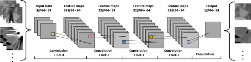
Architecture of the convolutional neural network for metal artifact reduction.

III. CNN-MAR METHOD

Because the proposed MAR approach is based on the CNN, it is referred to as CNN-MAR method. It consists of five steps: (1) metal trace segmentation; (2) artifact reduction with the LI and BHC; (3) artifact reduction with the trained CNN; (4) generation of a CNN prior image using tissue processing; (5) replacement of metal-affected projections with the forward projection of CNN prior, followed by the FBP reconstruction. The workflow of CNN-MAR is summarized in Fig. 4. Steps 1 and 5 are the same as our previous work [24], and step 2 has been described in the above subsection. Hence, we only provide the details for the key steps 3 and 4 as follows.

Fig. 4.

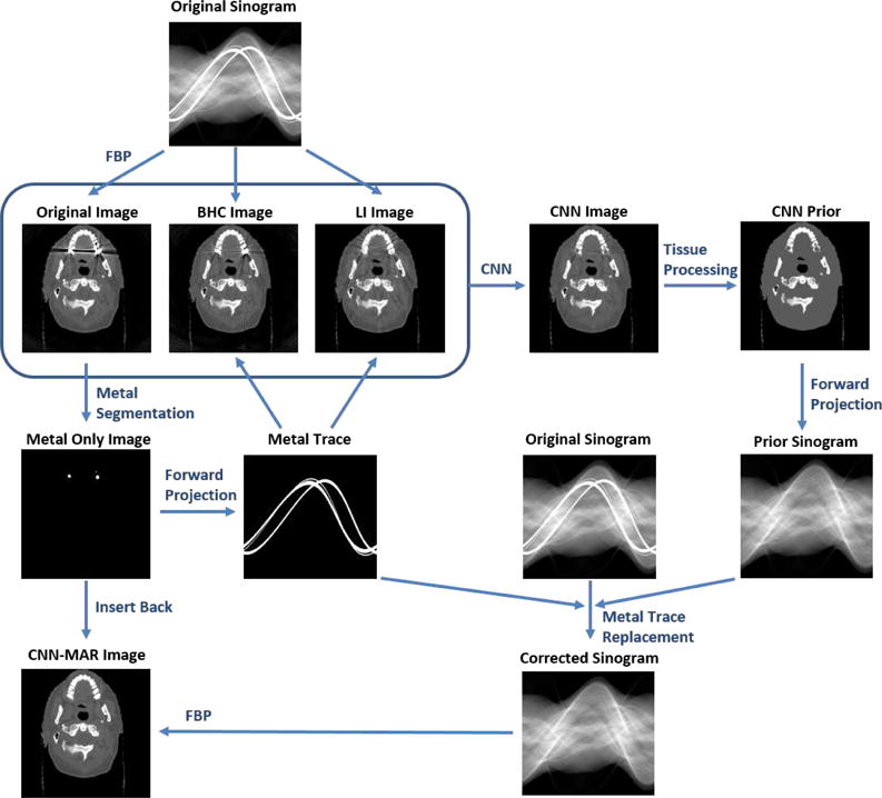
Flowchart of the proposed CNN-MAR method.

A. CNN Processing

After the BHC and LI corrections, the original uncorrected image x^art, BHC image x^BHC and LI image x^LI are combined as a three-channel image x^input. Hence, the image after CNN processing is

$${\mathbf{x}}^{\mathit{CNN}}=C_L({\mathbf{x}}^{\mathit{input}}),$$ (16)

where the parameters in C_L have been obtained in advance in the CNN training phase. Fig. 5 shows an example of the CNN inputs and processed CNN image. All the three input images contain obvious artifacts, as indicated by the arrows 1–3. Although the LI alleviates the artifacts indicated by the arrow 1, it introduces new artifacts indicated by the arrow 4. In the CNN image, the artifacts are remarkably suppressed.

Fig. 5.

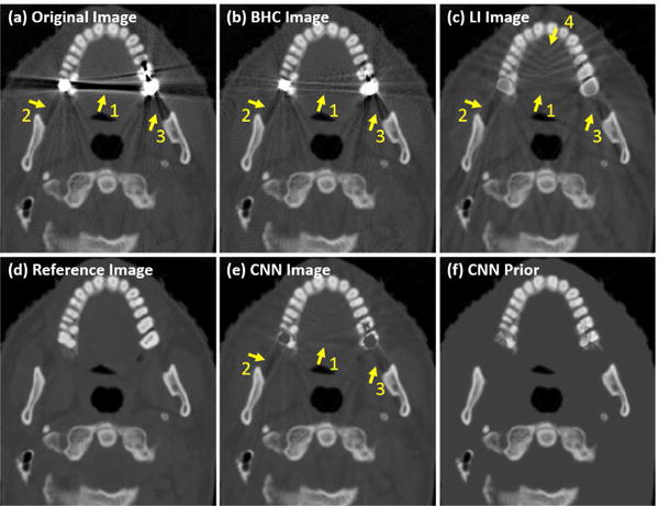
Illustration of the CNN image and CNN prior.

B. Tissue Processing

Although the metal artifacts are significantly reduced after the CNN processing, the remaining artifacts are still considerable. We generate a prior image from the CNN image by the proposed tissue processing approach. Because the water equivalent tissues have similar attenuations and are accounted for a dominate proportion in a patient, we assign these pixels with a uniform value to remove most of the artifacts and obtain a CNN prior image.

By the k-means clustering on the CNN image, two thresholds are automatically determined and the CNN image is segmented into bone, water and air. To avoid wrong clustering in the case of only a few bone pixels, the bone-water threshold is not less than 350 HU. Additionally, to preserve low-attenuated bones, larger regions are segmented with half of the bone-water threshold, and those regions overlapped with the previously obtained bony regions are also assumed as bone and preserved. Then, we obtain a binary image B for water regions with the target pixels setting to be one and the rest setting to be zero.

Because it may cause discontinuities at boundary and produce fake edges/structures to directly set all water regions with a constant value [13], [24], we introduce an N = 5 pixel transition between water and other tissues. Based on the binary image B, we introduce a distance image D, where the pixel value is set to be the distance between this pixel and its nearest zero pixel if the distance is not greater than N, and is set to be N if it is greater than N. Hence, in the image D, most of the water pixels are with the value N, and there is an N pixel transition region, while the other tissues are still zeros. We compute the weighted average of water pixel values:

$${\overline{x}}^{\mathit{CNN},w}=\frac{{\displaystyle {\sum }_i{D}_i{x}_i^{\mathit{CNN}}}}{{\displaystyle {\sum }_i{D}_i}},$$ (17)

Thus, the prior image is obtained:

$$x_i^{\mathit{prior}}=\frac{D_i}{N}{\overline{x}}^{\mathit{CNN},w}+(1-\frac{D_i}{N})x_i^{\mathit{CNN}}.$$ (18)

Finally, to avoid the potential discontinuities at boundaries of metals, the metal pixels are replaced with their nearest pixel values.

Fig. 5(f) shows an example of the CNN prior image after the tissue processing. It is clear that the regions of water equivalent tissue are flat and the artifacts are removed. Simultaneously, the bony structures are persevered very well. The CNN prior is beneficial for the projection interpolation. As shown in Fig. 6, the LI is a poor estimation of the missing projections. With the help of forward projection of the CNN prior, the surrogate sinogram is extremely close to the ideal one.

Fig. 6.

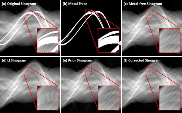
Comparison of sinogram completion. An ROI is enlarged and displayed with a narrower window.

IV. Experiments

A. Creating a Metal Artifact Database

74 metal-free CT images and 15 metal shapes are collected. Various metal implants are simulated, such as dental fillings, spine fixation screws, hip prostheses, coiling, wires, etc. The metal materials include titanium, iron, copper and gold. We carefully adjust the sizes, angles, positions and inserted metal materials so that the simulations are close to clinical cases. In this work, a database is created with 100 cases.

To segment water and bone from a benchmark image, thresholds T₁ and T₂ are set to linear attenuation coefficients corresponding to 100 HU and 1500 HU, respectively. Mass attenuation coefficients of water, bone and metals are obtained for the XCOM database [45]. To simulate metal-free and metal-inserted data, an equi-angular fan-beam geometry is assumed. A 120 kVp x-ray source is simulated and each detector bin is expected to receive 2 × 10⁷ photons in the case of blank scan [46]. There are 984 projection views over a rotation and 920 detector bins in a row. The distance between the x-ray source and the rotation center is 59.5 cm. The metal-free and metal-inserted images are reconstructed by the FBP from simulated sinograms and each image consists of 512 × 512 pixels.

B. CNN Training

In Fig.3, the convolutional kernel is 3 × 3 in each layer. Therefore, the convolutional weights are 3 × 3 × 3 × 32 in the first layer, 3 × 3 × 32 × 32 in the second to the fourth layers and 3 × 3 × 32 × 1 in the last layer. We set the padding to 1 in each layer so that the size of the output image is the same as the input.

To train the CNN, images are selected from the database to generate the training data. 10,000 patch samples with the size of 64 × 64 are extracted from the selected images. Because the spatial distribution of metal artifacts in an image is not uniform, we design a specific strategy to select training patches. A major proportion of the total training data are those patches with strongest artifacts in each corrected image, and the rest patches are randomly selected. The trained neural networks are very similar with different proportions between 50% to 80%. The obtained training data are randomly divided into two groups. 80% of the data is used for training and the rest is for validation during the CNN training. The CNN is implemented in Matlab with the MatConvNet toolbox [47], [48]. A GeForce GTX 970 GPU is used for acceleration. The training code runs about 25.5 hours and stops after 2000 iterations.

C. Numerical Simulation

Three typical metal artifacts cases are selected from the database to evaluate the usefulness of the proposed method. They are: case 1, two hip prostheses; case 2, two fixation screws and a round metal inserted in bone; case 3, several dental fillings. These cases are not used in the CNN training.

The proposed method is compared to the BHC, LI and a famous prior image based method NMAR [14]. In the NMAR, a prior image is generated from an original image in the case of smaller metal objects of medium density and from an LI image in the case of strong artifacts. For a comprehensive comparison, we generate prior images from both of the original and LI images for the NMAR, which are referred as to NMAR1 and NMAR2 in this paper, respectively. For a quantitative evaluation, we use the metal-free images as references to compute the root mean square error (RMSE) and the structural similarity (SSIM) index [49].

D. Real Data

The effectiveness of the proposed method is also validated over a clinical data. A patient with a surgical clip is scanned on a Siemens SOMATOM Sensation 16 CT scanner with 120 kVp and 496 mAs using the helical scanning geometry [50]. The measurement was acquired with 1160 projection views over a rotation and 672 detector bins in a row. The FOV is 25 cm in radius and distance from the x-ray source to the rotation center is 57 cm.

V. Results

A. Numerical Simulation

Fig. 7 shows the reference, uncorrected and corrected images of the bilateral hip prostheses case. The corresponding prior images for the NMAR1, NMAR2 and CNN-MAR are given in Fig. 8. A severe dark strip presents between two hip prostheses in the original image as indicated by the arrow “1”. Although the BHC alleviates these artifacts to some extent, the remaining artifacts are still remarkable. The NMAR1 corrected image also contains strong dark strip in the same location, which is due to its poor prior image. The NMAR method adopts a simple thresholding to segment air, water equivalent tissue, and bone after the image is smoothed with a Gaussian filter [14]. Then, air and water regions are set to −1000 HU and 0 HU, respectively. Because of the severe artifacts in the original image, several regions are segmented as wrong tissue types. The NMAR1 prior presents false structures as indicated by the arrows “1” and “2” in Fig. 8(a). The false structural information is propagated to the NMAR1 corrected image. The LI corrected image has moderate artifacts compared to the aforementioned methods. However, the bony structures near the metals, as highlighted in the magnified ROI, are blurred and distorted. This is due to the significant information loss near a large metal. As a result, the NMAR2 prior does not suffer from the wrong segmentation but an inaccurate bony structure as indicated by the arrow “3” in Fig. 8(b). Hence, the NMAR2 corrected images reduce artifacts well and introduce wrong bony structures. By comparison, the CNN image captures tissue structures faithfully from the original, BHC and LI images, and avoids most of the artifacts. Due to the excellent image quality of the CNN image, a good CNN prior is generated, followed by a CNN-MAR image with superior image quality. It is clearly seen from Fig. 7(h) that the artifacts are almost removed completely and the tissue features in the vicinity of metals are faithfully preserved.

Fig. 7.

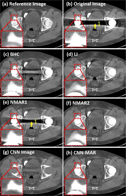
Case 1: bilateral hip prostheses. (a) is the reference image, (b) is the original uncorrected image, and (c)–(h) are the corrected results by the BHC, LI, NMAR1, NMAR2, CNN and CNN-MAR, respectively. The ROI highlighted by the small square is magnified. The display window is [−400 400] HU.

Fig. 8.

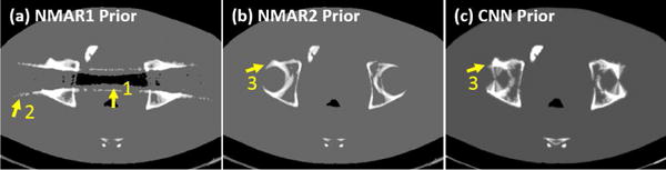
The prior images for NMAR1, NMAR2 and CNN-MAR in Fig. 7.

Fig. 9 presents the case 2, where two fixation screws and a metal are inserted in the shoulder blade. The metal artifacts in the original image are moderate, and the BHC is able to remove the bright artifacts (arrow “2”) around the metals and recovered some bony structures. On the contrary, the LI introduces many new artifacts, and most of the bony structures near the metals are lost as indicated by the arrow “1”. Both the NMAR1 and NMAR2 are not able to obtain satisfactory results because it can hardly get a good prior image from the original or LI corrected images. The CNN image restores most of the bony features near the metals, and no new artifacts are introduced. Consequently, the CNN-MAR corrected image is very close to the reference.

Fig. 9.

Same as Fig. 7 but for case 2: two fixation screws and a metal inserted in the shoulder blade. The display window is [−360 310] HU.

Fig. 10 shows the dental images with multiple dental fillings. The original, BHC, LI and NMAR1 images suffer from severe artifacts, and the NMAR2 has less artifacts. Although none of Figs. 10(b)–10(d) has a good image quality, the CNN demonstrates an outstanding capacity to preserve the tissue features and avoid most of the strong artifacts simultaneously. Consistent with the previous cases, the CNN-MAR achieves the best image quality.

Fig. 10.

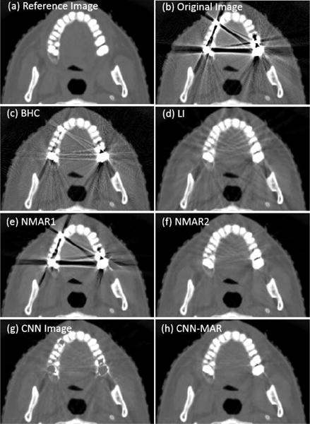
Same as Fig. 7 but for case 3: four dental fillings. The display window is [−1000 1400] HU.

Table I lists the RMSEs of the original and corrected images with respect to the reference images, where the metallic pixels are excluded. Because the noise also contributes to the RMSE, the artifact induced error is slightly smaller than the values listed in the table. The BHC, LI and NMAR1 have overall large error. In comparison, the NMAR2 achieves a higher accuracy. The CNN images have comparable accuracy to the NMAR2, and the CNN-MAR achieves the smallest RMSEs for all these three cases.

TABLE I.

RMSE of each image in the numerical simulation study. (Unit: HU).

	Original	BHC	LI	NMAR1	NMAR2	CNN	CNN-MAR
Case 1	155.0	86.3	46.2	121.2	35.4	33.1	29.1
Case 2	71.5	44.4	54.5	50.4	41.4	31.5	22.8
Case 3	320.3	183.5	107.3	234.9	82.3	83.4	58.4

Because the SSIM measures the structural similarity between two images, it is good to evaluate the strength of artifacts [49]. The SSIM index lies between 0 and 1, and a higher value means better image quality. Table II lists the SSIM of each image in the numerical simulation study. The BHC has comparable SSIM indices to those of the uncorrected images. The other five MAR methods increase the SSIM significantly. For the LI, NMAR1, NMAR2 and CNN, their ranks are case-dependent. Generally speaking, the NMAR2 and CNN have better image quality. By comparison, the CNN-MAR has the highest SSIM for the three cases, implying its superior and robust artifact reduction capability.

TABLE II.

SSIM of each image in the numerical simulation study.

	Original	BHC	LI	NMAR1	NMAR2	CNN	CNN-MAR
Case 1	0.565	0.576	0.576	0.887	0.935	0.940	0.943
Case 2	0.883	0.854	0.931	0.955	0.950	0.965	0.977
Case 3	0.522	0.536	0.886	0.833	0.942	0.932	0.967

B. Clinical Application

Fig. 11 shows a patient’s head CT image with a surgical clip. The patient is a 59 year-old female with diffused subarachnoid hemorrhage in the basal cisterns and sylvian fissures. The CT angiography demonstrates a left middle cerebral artery aneurysm. She is taken to the operation room and the aneurysm is clipped. She has numerous head CT scans after the surgery for assessment of increased intracranial pressure to rule out rebleeding and hydrocephalus [50]. The original, BHC and LI images contain too strong artifacts to provide bleeding information in her brain. The NMAR1 and NMAR2 are able to better alleviate artifacts. However, there still exists obvious artifacts in the images as indicated by the arrow “1”, and bony structures indicated by the arrow “2” are distorted. In comparison, the CNN-MAR achieves the best image quality. As highlighted in the rectangular region, there is only one tiny dark streak, and the bright hemorrhage can be observed clearly. The CNN-MAR demonstrates a superior metal artifact reduction and the potential for diagnostic tasks after the clipping surgery.

Fig. 11.

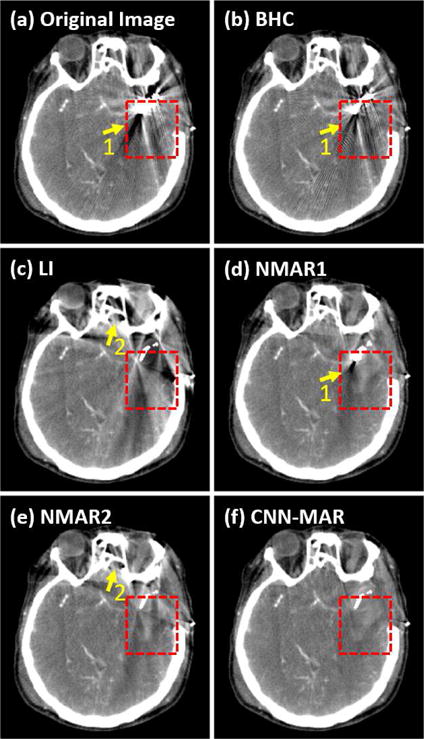
The head CT image with a surgical clip. (a) is the original uncorrected image, and (b)–(f) are the corrected results by the BHC, LI, NMAR1, NMAR2 and CNN-MAR, respectively. The display window is [−100 200] HU.

C. Properties of the Proposed CNN-MAR

1) Effectiveness of the Tissue Processing

To study the effectiveness of the tissue processing, we ignore the tissue processing step and directly assume the CNN images as the prior images. The corresponding corrected images are shown in Fig. 12. Compared to the CNN images in Figs. 7, 9 and 10, some artifacts can be alleviated by the forward projection. Nevertheless, most of the streaks that are tangent to the metals are preserved as indicated by the arrows in Fig. 12. By comparison, the tissue processing keeps the major structures and removes the low-contrast features and remaining artifacts. Although the features in the regions of water equivalent tissues are lost after the tissue processing, because the metal-affected projections account for a very small proportion in the sinogram, the missing information is able to be partially recovered from the rest of the unaffected projections. In addition, in the projection replacement step, a projection transition is applied to compensate for the difference between the prior sinogram and the measurements at the boundary of the metal traces [24], which is also beneficial to the information recovery. However, in the presence of large metals, a low-contrast feature in the vicinity of metal may suffer from missing or distortion.

Fig. 12.

Results obtained by directly adopting a CNN image as the prior image without the tissue processing step. (a)–(c) corresponds to the cases 1–3, respectively.

2) Selection of Input Images (MAR Methods)

In this work, the original uncorrected, BHC and LI images are adopted as the input of CNN. We also compare the results with various input images (MAR methods). Here, we apply the original uncorrected, BHC, LI, NMAR1 and NMAR2 images as a five-channel input image, and adopt the original and LI images as a two-channel input image. In addition, the NMAR2 images is employed as a one-channel input image. Fig. 13 shows the results of dental fillings case. When NMAR2 is selected as the single input image, the CNN processing is equivalent to the NMAR-CNN method proposed by Gjesteby et al. [31], [35]. Because the NMAR2 image has less artifacts, the CNN image and CNN-MAR image have better image quality. Regarding the multi-channel input, it can be seen from the top three rows that the performance of artifacts reduction is improved by introducing more input images. Particularly, compared to the cases of two-channel input images, three-channel input images remarkably improve the image quality. Therefore, introducing the NMAR1 and NMAR2 only brings limited benefits. This effect depends on if the newly introduced input images contain new useful information. As the aforementioned, the BHC and LI belong to different MAR strategies, which provide complementary information. Without the BHC, some artifacts are wrongly classified as tissue structures and preserved, as illustrated in the third row of Fig. 13. On the contrary, the NMAR1 and NMAR2 are obtained based on prior images from the original and LI images, respectively. Hence, they provide limited new information. In summary, as an open MAR framework, the performance of CNN-MAR can be further improved in the near future by incorporating various types of MAR algorithms.

Fig. 13.

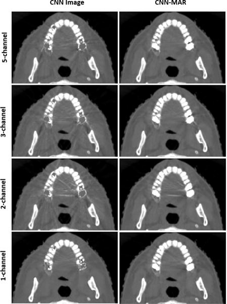
CNN and CNN-MAR results based on different channels of input images. Five-channel: original, BHC, LI, NMAR1 and NMAR2 images. Three-channel (default): original, BHC and LI images. Two-channel: original and LI images. One-channel: NMAR2 image.

3) Architecture of the CNN

To study the performance of CNN with respect to different architectures, we adjust the CNN parameters and calculate the average RMSE and SSIM over ten simulated metal artifact cases including the aforementioned three cases. Fig. 14 shows the values of RMSE and SSIM using the networks with different number of convolutional layers, number of filters per layer, and the size of each filter. In each subplot, there is only one parameter to be tuned and other parameters are kept as the default ones. The number of neurons in the network increases with the increase of these three parameters, obtaining slightly smaller RMSE and greater SSIM indices. However, because the computational cost rises considerably by using greater parameters, we employ a medium size CNN in this work.

Fig. 14.

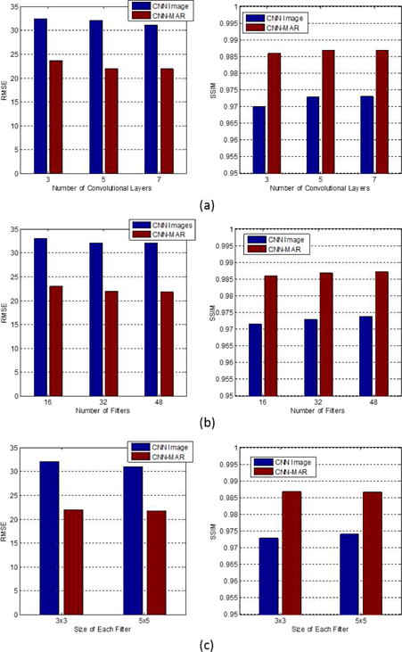
Average RMSE and SSIM of CNN images and CNN-MAR images with respect to various CNN architecture parameters: (a) number of convolutional layers, (b) number of filters/features in each layer and (c) the size of each filter. The default CNN has 5 convolutional layers, 32 filters per layer, and each filter is with the size of 3 × 3.

4) Training Data

We compare the network trained with different numbers of patches. Fig. 15 presents the average RMSE and SSIM values over ten cases of our results using the network trained with 100, 500, 2000 and 10000 patches. It is clear that the RMSE decreases and the SSIM increases dramatically by applying more training data. This suggests that the performance of the proposed method strongly depends on the size of training data.

Fig. 15.

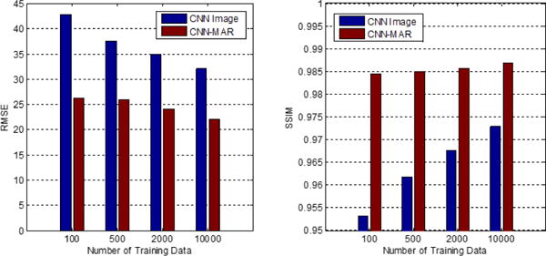
Average RMSE and SSIM values using the CNN trained with different data size.

We also compare selection strategies for the training data. The convergence curves of CNN training are presented in Fig. 16(a), and the obtained network after 2000 training epochs is used in this work. It can be observed that the energy of the objective function decreases steadily with the increasing training epoch. In Fig. 16(a), the training and validation data are selected from a subset of the same dataset, which consists of all types of inserted metals. It is clear that the trained CNN works well on the validation data. In Fig. 16(b), the training data and the validation data are selected from the same subset. While the training data is from all types of metals except the multiple dental fillings, and the validation data is from the multiple dental fillings cases. The two separated curves demonstrate an unsatisfactory performance of the obtained CNN on the validation data caused by the difference of the artifact patterns in the two data sets. Hence, it is crucial to include a wider variety of metal artifacts cases as the training data.

Fig. 16.

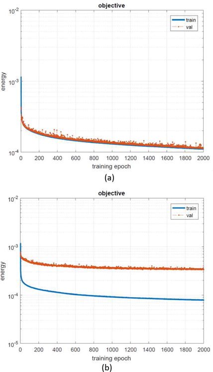
The convergence curves of CNN training in terms of energy of loss function versus training epochs. (a) Training data and validation data are selected from the same dataset. (b) Training data and validation data are from different cases in the dataset.

5) Training Epochs

The proposed method is tested with different training epochs. Fig. 17 compares average RMSE and SSIM values over ten cases of the CNN and CNN-MAR images obtained with the network after 100, 200, 1000 and 2000 training epochs. Obviously, by increasing the training epochs, the RMSE of CNN images decreases steadily and the SSIM increases constantly. After the tissue processing, the image quality of CNN-MAR images is remarkably improved. Likewise, the RMSE and SSIM of CNN-MAR images with respective to training epochs follows the same trend to those of CNN images.

Fig. 17.

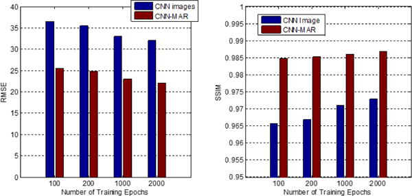
Average RMSE and SSIM values using the CNN trained after different epochs.

VI. Discussion And Conclusion

From the aforementioned experimental results, it can be seen that the CNN and tissue processing are two mutual beneficial steps. For the CNN step, its strength is to fuse useful information from different sources to avoid strong artifacts. Its drawback is that the CNN can hardly remove all artifacts and mild artifacts typically remain. As to the tissue processing, similar to other prior image based MAR methods, it can remove moderate artifacts and generate a satisfactory prior image. However, in the presence of severe artifacts, the prior image usually suffers from misclassification of tissues. By incorporating the CNN and tissue processing, the CNN training can stop with fewer epochs, and the obtained CNN prior is not affected by tissue misclassification. Their strengths are complementary.

The key factors to ensure outstanding performance of the CNN-MAR are twofold: selection of the appropriate MAR methods and preparation of the training data. The former factor provides sufficient information for the CNN to distinguish tissue structures from the artifacts. The later ensures the generality of the trained CNN by involving as many varieties of metal artifacts cases as possible.

The forward projection of metal identifies which project data is affected. For data correction/estimation based metal artifact reduction methods, including the proposed method, the performance of artifact reduction may be compromised in the case of inaccurate metal segmentation [51]. Fortunately, a few advanced metal segmentation schemes have been reported [50], [52], which can be directly applied to the proposed method. Moreover, the deep learning strategy has been widely used for image segmentation [53]. Study of applying the neural network for the robust metal segmentation is planned for our future work.

Although the proposed CNN-MAR in this paper works on 2D image slices, it can be directly extended to 3D volumetric images. Along the new dimension, due to different spatial distribution patterns of tissue structures and artifacts, the 3D version may achieve superior performance. Meanwhile, 3D data will require more training time.

In conclusion, we have proposed a convolutional neural network based metal artifact reduction (CNN-MAR) framework. It is an open artifact reduction framework that is able to distinguish tissue structures from artifacts and fuse the meaningful information to yield a CNN image. By applying the designed tissue processing technique, a good prior is generated to further suppress artifacts. Both numerical simulations and clinical application have demonstrated that the CNN-MAR can significantly reduce metal artifacts and restore fine structures near the metals to a large extent. In the future, we will increase the training data and involve more MAR methods in the CNN-MAR framework to improve its capability. From a broader aspect, the proposed framework has a great potential for other artifacts reduction problems in the biomedical imaging and industrial applications.

References

- 1.De Man B, Nuyts J, Dupont P, Marchal G, Suetens P. Metal streak artifacts in x-ray computed tomography: A simulation study. IEEE Transactions on Nuclear Science. 1999;46(3):691–696. [Google Scholar]
- 2.Gjesteby L, De Man B, Jin Y, Paganetti H, Verburg J, Giantsoudi D, Wang G. Metal artifact reduction in CT: where are we after four decades? IEEE Access. 2016;4:5826–5849. [Google Scholar]
- 3.Jessie YH, James RK, Jessica LN, Xinming L, Peter AB, Francesco CS, David SF, Dragan M, Rebecca MH, Stephen FK. An evaluation of three commercially available metal artifact reduction methods for CT imaging. Physics in Medicine & Biology. 2015;60(3):1047–1067. doi: 10.1088/0031-9155/60/3/1047. [DOI] [PMC free article] [PubMed] [Google Scholar]
- 4.Mouton A, Megherbi N, Van Slambrouck K, Nuyts J, Breckon TP. An experimental survey of metal artefact reduction in computed tomography. Journal of X-ray Science and Technology. 2013;21(2):193–226. doi: 10.3233/XST-130372. [DOI] [PubMed] [Google Scholar]
- 5.Park HS, Hwang D, Seo JK. Metal artifact reduction for polychromatic x-ray CT based on a beam-hardening corrector. IEEE Transactions on Medical Imaging. 2016;35(2):480–487. doi: 10.1109/TMI.2015.2478905. [DOI] [PubMed] [Google Scholar]
- 6.Hsieh J, Molthen RC, Dawson CA, Johnson RH. An iterative approach to the beam hardening correction in cone beam CT. Medical Physics. 2000;27(1):23–29. doi: 10.1118/1.598853. [DOI] [PubMed] [Google Scholar]
- 7.Zhang Y, Mou X, Tang S. Beam hardening correction for fan-beam CT imaging with multiple materials. in 2010 IEEE Nuclear Science Symposium and Medical Imaging Conference (2010 NSS/MIC) 2010:3566–3570. [Google Scholar]
- 8.Kachelrieß M, Watzke O, Kalender WA. Generalized multidimensional adaptive filtering for conventional and spiral single-slice, multi-slice, and cone-beam CT. Medical physics. 2001;28(4):475–490. doi: 10.1118/1.1358303. [DOI] [PubMed] [Google Scholar]
- 9.Mehranian A, Ay MR, Rahmim A, Zaidi H. X-ray CT metal artifact reduction using wavelet domain L0 sparse regularization. IEEE Transactions on Medical Imaging. 2013;32(9):1707–1722. doi: 10.1109/TMI.2013.2265136. [DOI] [PubMed] [Google Scholar]
- 10.Zhang Y, Pu Y-F, Hu J-R, Liu Y, Chen Q-L, Zhou J-L. Efficient ct metal artifact reduction based on fractional-order curvature diffusion. Computational and Mathematical Methods in Medicine. 2011;2011:173748. doi: 10.1155/2011/173748. [DOI] [PMC free article] [PubMed] [Google Scholar]
- 11.Zhang Y, Pu Y-F, Hu J-R, Liu Y, Zhou J-L. A new ct metal artifacts reduction algorithm based on fractional-order sinogram inpainting. Journal of X-ray science and technology. 2011;19(3):373–384. doi: 10.3233/XST-2011-0300. [DOI] [PubMed] [Google Scholar]
- 12.Kalender W, Hebel R, Ebersberger J. Reduction of CT artifacts caused by metallic implants. Radiology. 1987;164(2):576. doi: 10.1148/radiology.164.2.3602406. [DOI] [PubMed] [Google Scholar]
- 13.Bal M, Spies L. Metal artifact reduction in CT using tissue-class modeling and adaptive prefiltering. Medical Physics. 2006;33(8):2852–2859. doi: 10.1118/1.2218062. [DOI] [PubMed] [Google Scholar]
- 14.Meyer E, Raupach R, Lell M, Schmidt B, Kachelrieß M. Normalized metal artifact reduction (NMAR) in computed tomography. Medical Physics. 2010;37(10):5482–5493. doi: 10.1118/1.3484090. [DOI] [PubMed] [Google Scholar]
- 15.Prell D, Kyriakou Y, Beister M, Kalender WA. A novel forward projection-based metal artifact reduction method for flat-detector computed tomography. Physics in Medicine and Biology. 2009;54(21):6575–6591. doi: 10.1088/0031-9155/54/21/009. [DOI] [PubMed] [Google Scholar]
- 16.Wang J, Wang S, Chen Y, Wu J, Coatrieux J-L, Luo L. Metal artifact reduction in ct using fusion based prior image. Medical Physics. 2013;40(8):081903. doi: 10.1118/1.4812424. [DOI] [PubMed] [Google Scholar]
- 17.Zhang Y, Mou X. Metal artifact reduction based on the combined prior image. arXiv preprint arXiv:1408.5198. 2014 [Google Scholar]
- 18.Wang G, Snyder DL, OSullivan JA, Vannier MW. Iterative deblurring for CT metal artifact reduction. IEEE Transactions on Medical Imaging. 1996;15(5):657–664. doi: 10.1109/42.538943. [DOI] [PubMed] [Google Scholar]
- 19.Wang G, Vannier MW, Cheng PC. Iterative x-ray cone-beam tomography for metal artifact reduction and local region reconstruction. Microscopy and Microanalysis. 1999;5(1):58–65. doi: 10.1017/S1431927699000057. [DOI] [PubMed] [Google Scholar]
- 20.Zhang X, Wang J, Xing L. Metal artifact reduction in x-ray computed tomography (CT) by constrained optimization. Medical Physics. 2011;38(2):701–711. doi: 10.1118/1.3533711. [DOI] [PMC free article] [PubMed] [Google Scholar]
- 21.Zhang Y, Mou X, Yan H. Weighted total variation constrained reconstruction for reduction of metal artifact in ct. in 2010 IEEE Nuclear Science Symposium and Medical Imaging Conference (2010 NSS/MIC) 2010:2630–2634. [Google Scholar]
- 22.Lemmens C, Faul D, Nuyts J. Suppression of metal artifacts in CT using a reconstruction procedure that combines map and projection completion. IEEE Transactions on Medical Imaging. 2009;28(2):250–260. doi: 10.1109/TMI.2008.929103. [DOI] [PubMed] [Google Scholar]
- 23.Zhang Y, Mou X. Metal artifact reduction based on beam hardening correction and statistical iterative reconstruction for x-ray computed tomography. in Proc SPIE 8668, Medical Imaging 2013: Physics of Medical Imaging. 2013;8668:86682O. [Google Scholar]
- 24.Zhang Y, Yan H, Jia X, Yang J, Jiang SB, Mou X. A hybrid metal artifact reduction algorithm for x-ray CT. Medical Physics. 2013;40(4):041910. doi: 10.1118/1.4794474. [DOI] [PubMed] [Google Scholar]
- 25.Wang G. A perspective on deep imaging. IEEE Access. 2016;4:8914–8924. [Google Scholar]
- 26.Jin KH, McCann MT, Froustey E, Unser M. Deep convolutional neural network for inverse problems in imaging. IEEE Transactions on Image Processing. 2017;26(9):4509–4522. doi: 10.1109/TIP.2017.2713099. [DOI] [PubMed] [Google Scholar]
- 27.Chen H, Zhang Y, Kalra MK, Lin F, Chen Y, Liao P, Zhou J, Wang G. Low-dose CT with a residual encoder-decoder convolutional neural network. IEEE transactions on medical imaging. 2017;36(12):2524–2535. doi: 10.1109/TMI.2017.2715284. [DOI] [PMC free article] [PubMed] [Google Scholar]
- 28.Wolterink JM, Leiner T, Viergever MA, Išgum I. Generative adversarial networks for noise reduction in low-dose CT. IEEE Transactions on Medical Imaging. 2017;36(12):2536–2545. doi: 10.1109/TMI.2017.2708987. [DOI] [PubMed] [Google Scholar]
- 29.Gjesteby L, Yang Q, Xi Y, Zhou Y, Zhang J, Wang G. Deep learning methods to guide CT image reconstruction and reduce metal artifacts. in SPIE Medical Imaging International Society for Optics and Photonics. 2017:101 322W–101 322W–7. [Google Scholar]
- 30.Chen H, Zhang Y, Zhang W, Liao P, Li K, Zhou J, Wang G. Low-dose CT via convolutional neural network. Biomedical Optics Express. 2017;8(2):679–694. doi: 10.1364/BOE.8.000679. [DOI] [PMC free article] [PubMed] [Google Scholar]
- 31.Gjesteby L, Yang Q, Xi Y, Claus B, Jin Y, Man BD, Wang G. Reducing metal streak artifacts in CT images via deep learning: Pilot results. in The 14th International Meeting on Fully Three-Dimensional Image Reconstruction in Radiology and Nuclear Medicine. 2017:611–614. [Google Scholar]
- 32.Du W, Chen H, Wu Z, Sun H, Liao P, Zhang Y. Stacked competitive networks for noise reduction in low-dose CT. PloS One. 2017;12(12):e0190069. doi: 10.1371/journal.pone.0190069. [DOI] [PMC free article] [PubMed] [Google Scholar]
- 33.Chen H, Zhang Y, Chen Y, Zhang J, Zhang W, Sun H, Lv Y, Liao P, Zhou J, Wang G. Learn: Learned experts assessment-based reconstruction network for sparse-data CT. IEEE Transactions on Medical Imaging. 2018 doi: 10.1109/TMI.2018.2805692. [DOI] [PMC free article] [PubMed] [Google Scholar]
- 34.Liu Y, Zhang Y. Low-dose CT restoration via stacked sparse denoising autoencoders. Neurocomputing. 2018;284:80–89. [Google Scholar]
- 35.Gjesteby L, Yang Q, Xi Y, Shan H, Claus B, Jin Y, Man BD, Wang G. Deep learning methods for CT image-domain metal artifact reduction. in SPIE Optical Engineering + Applications. 2017;10391:103910W. SPIE. [Google Scholar]
- 36.Zhang Y, Chu Y, Yu H. Reduction of metal artifacts in x-ray CT images using a convolutional neural network. in SPIE Optical Engineering + Applications. 2017;10391:103910V. [Google Scholar]
- 37.Zhang Y, Yu H. Convolutional neural network based metal artifact reduction in x-ray computed tomography. arXiv preprint arXiv:1709.01581. 2017 doi: 10.1109/TMI.2018.2823083. [DOI] [PMC free article] [PubMed] [Google Scholar]
- 38.Park HS, Chung YE, Lee SM, Kim HP, Seo JK. Sinogram-consistency learning in CT for metal artifact reduction. arXiv preprint arXiv:1708.00607. 2017 [Google Scholar]
- 39.Park HS, Lee SM, Kim HP, Seo JK. Machine-learning-based nonlinear decomposition of CT images for metal artifact reduction. arXiv preprint arXiv:1708.00244. 2017 [Google Scholar]
- 40.AAPM. 2016 http://www.aapm.org/GrandChallenge/LowDoseCT/
- 41.Kyriakou Y, Meyer E, Prell D, Kachelrieß M. Empirical beam hardening correction (EBHC) for CT. Med Phys. 2010;37(10):5179–5187. doi: 10.1118/1.3477088. [DOI] [PubMed] [Google Scholar]
- 42.Elbakri I, Fessler J. Statistical image reconstruction for polyenergetic x-ray computed tomography. IEEE Transactions on Medical Imaging. 2002;21(2):89–99. doi: 10.1109/42.993128. [DOI] [PubMed] [Google Scholar]
- 43.Xu Q, Yu HY, Mou XQ, Zhang L, Hsieh J, Wang G. Low-dose x-ray CT reconstruction via dictionary learning. Medical Imaging, IEEE Transactions on. 2012;31(9):1682–1697. doi: 10.1109/TMI.2012.2195669. [DOI] [PMC free article] [PubMed] [Google Scholar]
- 44.Verburg JM, Seco J. CT metal artifact reduction method correcting for beam hardening and missing projections. Physics in Medicine and Biology. 2012;57(9):2803–2818. doi: 10.1088/0031-9155/57/9/2803. [DOI] [PubMed] [Google Scholar]
- 45.Berger M, Hubbell J, Seltzer S, Chang J, Coursey J, Sukumar R, Zucker D. XCOM: Photon cross sections database. 1998 [Online]. Available: http://www.nist.gov/pml/data/xcom/index.cfm.
- 46.Tang S, Mou X, Yang Y, Xu Q, Yu H. Application of projection simulation based on physical imaging model to the evaluation of beam hardening corrections in x-ray transmission tomography. Journal of X-Ray Science and Technology. 2008;16(2):95–117. [Google Scholar]
- 47.Vedaldi A, Lenc K. Matconvnet: Convolutional neural networks for matlab. in Proceedings of the 23rd ACM international conference on Multimedia. 2015:689–692. [Google Scholar]
- 48.MatConvNet: CNNs for MATLAB. 2017 [Online]. Available: http://www.vlfeat.org/matconvnet/
- 49.Wang Z, Bovik A, Sheikh H, Simoncelli E. Image quality assessment: From error visibility to structural similarity. Image Processing, IEEE Transactions on. 2004;13(4):600–612. doi: 10.1109/tip.2003.819861. [DOI] [PubMed] [Google Scholar]
- 50.Yu HY, Zeng K, Bharkhada DK, Wang G, Madsen MT, Saba O, Policeni B, Howard MA, Smoker WRK. A segmentation-based method for metal artifact reduction. Academic Radiology. 2007;14(4):495–504. doi: 10.1016/j.acra.2006.12.015. [DOI] [PMC free article] [PubMed] [Google Scholar]
- 51.Stille M, Kratz B, Mller J, Maass N, Schasiepen I, Elter M, Weyers I, Buzug TM. Influence of metal segmentation on the quality of metal artifact reduction methods. SPIE Med Imaging. 2013:86683. [Google Scholar]
- 52.Hegazy MAA, Cho MH, Lee SY. A metal artifact reduction method for a dental CT based on adaptive local thresholding and prior image generation. BioMedical Engineering OnLine. 2016;15(1):119. doi: 10.1186/s12938-016-0240-8. [DOI] [PMC free article] [PubMed] [Google Scholar]
- 53.He K, Zhang X, Ren S, Sun J. Deep residual learning for image recognition. in Proceedings of the IEEE Conference on Computer Vision and Pattern Recognition. 2016:770–778. [Google Scholar]