Intelligent Parameter Tuning in Optimization-based Iterative CT Reconstruction via Deep Reinforcement Learning

Abstract

A number of image-processing problems can be formulated as optimization problems. The objective function typically contains several terms specifically designed for different purposes. Parameters in front of these terms are used to control the relative importance among them. It is of critical importance to adjust these parameters, as quality of the solution depends on their values. Tuning parameters is a relatively straightforward task for a human, as one can intuitively determine the direction of parameter adjustment based on the solution quality. Yet manual parameter tuning is not only tedious in many cases, but becomes impractical when a number of parameters exist in a problem. Aiming at solving this problem, this paper proposes an approach that employs deep reinforcement learning to train a system that can automatically adjust parameters in a human-like manner. We demonstrate our idea in an example problem of optimization-based iterative CT reconstruction with a pixel-wise total-variation regularization term. We set up a Parameter-Tuning Policy Network (PTPN), which maps a CT image patch to an output that specifies the direction and amplitude by which the parameter at the patch center is adjusted. We train the PTPN via an end-to-end reinforcement learning procedure. We demonstrate that under the guidance of the trained PTPN, reconstructed CT images attain quality similar or better than those reconstructed with manually tuned parameters.

I. Introduction

A number of medical image-processing problems can be formulated as solving optimization problems. In such problems, the objective function typically contain several terms carefully designed for different purposes. A set of parameters are used to control the relative weights of these terms in order to achieve a satisfactory solution quality. Take a typical problem of iterative Computed Tomography (CT) reconstruction as an example, it can be formulated as

$$f^{\ast }=\arg \underset{f}{min}\frac{1}{2}{\left|Pf-g\right|}^2+\mathrm{\lambda }R[f],$$ (1)

where f^∗ is the image to be reconstructed by solving the optimization problem, P stands for the x-ray projection operator, and g the measured projection data. The first data-fidelity term ensures agreement between f^∗ and the measurement g. R[f] stands for a regularization term specifically designed to enforce quality of the solution image from a certain aspect, e.g. piece-wise smoothness. λ is the parameter that is used to control the trade-off between this regularization term and the data-fidelity term. Over the years, a number of regularization terms have been developed to successfully restore a high-quality solution f^∗ using undersampled or noisy measurement g. Examples include, but are not limited to, total variation (TV) [1]–[3], tight frame (TF) [4], [5], and nonlocal means (NLM) [6]–[8].

Despite the success, parameter tuning in these optimization-based image processing problems is inevitable. Manual adjustment of the parameters for the best image quality is not uncommon in literature [2], [3], [5], [7], [8]. Yet this is a tedious approach, as one has to carefully navigate through the parameter space to find the optimal value. The required efforts and human time impede real applications of those novel image-processing methods. Moreover, manual parameter tuning becomes increasingly challenging in those problems with multiple regularization terms. An extreme example is the CT reconstruction problem but with pixel-wise weighting parameters [9], [10]. Clearly, the substantial amount of parameters makes manual parameter tuning infeasible. Therefore, it is highly desirable to develop a method for automatic parameter adjustment. Over the years, this problem has attracted a lot of research interests. For instance, generalized cross validation and L-curve methods have been used to choose the regularization parameters [11]–[13]. It has been proposed to develop a method to assess image quality, which can then be used as guidance for parameter adjustment [14], [15]. In certain contexts, such as the CT reconstruction problem, it may be possible to estimate the level of data contamination based on physics or mathematical principles. This can provide valuable information to set the parameter values [16]. In the context of prior-image based image reconstruction, a novel method to estimate the optimal parameter value has also been proposed [17]. Despite these efforts, a practical solution that is applicable to general problems still does not exist, calling for further investigations.

Although it is quite difficult for a computer to automate the parameter-tuning process, this task seems to be less of a problem for humans. One typically has a strong intuition about which direction the parameter should be adjusted based on the observed image quality. Again, let us take the iterative CT reconstruction problem in Eq. (1) as an example. By looking at the solution image, one knows that the regularization strength needs to be increased, if the solution appears to be noisy, or be reduced otherwise. Based on this fact, it is of interest and importance to model this remarkable intuition and capability in an intelligence system, which can then be used to solve the parameter-tuning problem from a new angle.

Recently, the tremendous success in deep-learning regime shines a light in this direction. In the past few years, deep learning has clearly demonstrated its power in numerous medical image processing problems [18]–[24]. More importantly, it was found that human-level intelligence can be spontaneously generated via deep-learning schemes, which enables a system to perform a certain task in a human-like fashion, or even better than humans. In a pioneering study, an artificial intelligence system was developed to realize human-level control of Atari computer games [25], [26]. Employing a deep Q-network approach, the system was trained through the framework of deep reinforcement learning to learn how to interact with the environment, i.e. play an Atari game. The results were remarkable: the trained system was able to achieve a level comparable to that of professional human players in a set of 49 Atari games.

Motivated by this fact, we propose in this paper to develop an intelligent system to accomplish the parameter-tuning task in optimization-based image-processing problems. We take a CT reconstruction problem as an example to demonstrate our idea. Specifically, we will develop a Parameter-Tuning Policy Network, which can intellectually determine the direction and magnitude of parameter adjustment by observing an input image patch. The rest of this paper is organized as follows. Sec. II will introduce the problem of TV-based CT reconstruction with pixel-wise regularization. We will also describe the PTPN structure and how to train it to develop the skill of parameter tuning. Sec. III will present our validation studies and results. Finally, we will make some discussions in Sec. IV and conclude the study in Sec. V.

II. Methods

A. CT reconstruction framework

In this paper, we consider the following iterative CT reconstruction problem:

$$f^{\ast }=\arg \underset{f}{min}\frac{1}{2}{\left|Pf-g\right|}^2+\left|\mathrm{\lambda }\cdot \nabla f\right|.$$ (2)

This approach falls into the regime of TV-based regularization [1], which penalizes the L₁ norm of the image gradient to ensure image smoothness while preserving edges. In the second term of the objective function, we consider a general case that extends λ into a vector. Each entry of λ controls the regularization strength at an image pixel. The substantially large amount of parameters in this example problem compared to a typical single-parameter TV model highlights the need for an automatic parameter-tuning system.

There are a number of novel numerical algorithms to solve this optimization problem for fixed parameters λ [27]–[29]. In this study, we use the alternating direction method of multipliers (ADMM) [29]. It introduces an auxiliary variable d to replace ∇f in the original problem and adds a constraint d = ∇f to guarantee the equivalence between the constrained problem and the original problem. Such a constraint is then integrated with the objective function by considering the augmented Lagrangian:

$$\begin{array}{c}\mathrm{ℒ}(f,d,\mathrm{\Gamma })=\frac{1}{2}{\left|Pf-g\right|}^2+\left|\mathrm{\lambda }\cdot d\right|+\frac{\beta }{2}{\left|\nabla f-d\right|}^2\\ +\langle \mathrm{\Gamma },\nabla f-d\rangle ,\end{array}$$ (3)

where β is a parameter of the algorithm. Γ denotes the Lagrangian multiplier which is used to guarantee the convergence of the algorithm. The original optimization problem is solved by alternatively tackling this augmented Lagrangian function with respect different variables. Major steps of the ADMM algorithm are outlined in Fig. 1. Due to the large scale of the reconstruction problem, the matrix inverse operation in Line 2 is achieved using the conjugate gradient algorithm [30].

Fig. 1.

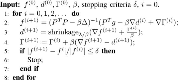
ADMM algorithm used to solve the problem in Eq. 2.

B. Parameter-tuning methodology

Let x denote the pixel position of the reconstructed image. If a human were asked to adjust parameter λ(x) in a trial-and-error fashion, he would repeatedly observe the reconstructed image quality under λ(x) and then decide how to change the parameters based on human intuition. This process would continue, until a satisfactory image is obtained. In this study, we propose to develop a parameter-tuning system to replace the human in this process.

Denote the parameter-tuning iteration step with k. At each step, the system observes the reconstructed image f^k generated by the image reconstruction system using the ADMM algorithm. Note that f^k is the solution at the convergence of the ADMM algorithm, rather than the intermediate image during the ADMM iteration. For each position x, the image patch centering at this pixel, denoted as S_fk (x) is fed to the parameter-tuning system. The system then outputs the direction and magnitude by which the parameter λ^k(x) is adjusted. Here, we explicitly associate λ(x) with the index k, as it will vary from step to step. Such a process continues, until a stopping criteria is met.

We would like to achieve automatic parameter-tuning capability via the Q-learning approach [31]. Specifically, Q-learning considers the optimal action-value function defined as

$$Q^{\ast }(s,a)=\underset{\pi }{max}[r^k+\gamma r^{k+1}+{\gamma }^2{r}^{k+2}+\cdots |s_k=s,a_k=a,\pi ],$$ (4)

where s is the observed system state, i.e. an image patch S_fk (x) in this study. a is the action taken, namely the way of adjusting parameter λ^k(x). We consider five possible actions: keeping the parameter λ^k(x) unchanged, increasing or decreasing it by 10%, and increasing or decreasing it by 50%. We arbitrarily choose the values of 50% or 10% as possible amounts of changes, as we expect these values will not critically affect the capability of parameter tuning of our system. r^k is the reward at step k based on a predefined reward function. In the specific problem here, the reward function is chosen to quantify the quality change of the reconstructed image after taking the action a. Specifically, improved image quality is assigned a positive reward, and otherwise a negative reward. γ ≤ 1 is a discount factor, and π stands for the parameter-tuning policy to be determined: taking an action a after observing a state s. Here, we consider a greedy policy that always selects the action maximizing the Q^∗ value under the input s, i.e. a = arg max_a′ Q^∗(s, a′). To determine this policy, it is necessary to establish the optimal action-value function Q^∗(s, a).

The explicit form of the action-value function is generally unknown. In this study, we parametrize this function using a convolutional neural network (CNN) Q(s, a; W), where W denotes the set of network parameters. This network is referred to as Parameter-Tuning Policy Network (PTPN) from hereon. The structure of the network is depicted in Fig. 2. The input of this network is a state s, namely an image patch. There are five output nodes corresponding to the five actions considered. The output value of PTPN at a node corresponding to an action a is the function value Q(s, a; W). Through a reinforcement learning process described in the next section, parameter set W of the optimal action-value function Q^∗(s, a; W) will be determined. After that, we can use this established function for parameter tuning. As such, since the policy is to select the action maximizing the Q^∗ function value, we use PTPN to calculate output values for the input s = S_fk (x) and adjust λ^k(x) by taking the action corresponding to the output node with the highest value.

Fig. 2.

Network structure of PTPN. The input is a patch cropped out of the solution image f^k. The five outputs are directions and magnitudes of changing the parameter at the patch center pixel. Number of units and data sizes at each layer are specified at the top. Connection between subsequent layers are also presented.

C. PTPN training via deep reinforcement learning

1) General deep reinforcement learning idea

One particular property of the Q^∗(s, a) function is the Bellman equation [32]:

$$Q^{\ast }(s,a)=r+\gamma \underset{a\prime }{max}{Q}^{\ast }(s\prime ,a\prime ),$$ (5)

where r is the reward achieved by the optimal action a based on the current state s. s^′ is the state that follows s after taking the action a. When the function Q^∗(s, a) is parameterized by a CNN, Q(s, a) ≈ Q(s, a; W), we can determine W by minimizing a loss function L(W) = [r + γ max_a′ Q(s′, a′; W) − Q(s, a; W)]², which essentially penalizes the deviation from the Bellman equation.

Following the standard approach of reinforcement learning [25], [26], we introduce another variable W′ and define a target term y = r + γ max_a′ Q(s′, a′; W′). For a fixed W′, we consider the loss function

$$L(W)={[y-Q(s,a;W)]}^2.$$ (6)

Note that the s′ inside the target term is related to s by the action a. We perform learning in a sequence of stages. In each stage, the parameter W′ is kept unchanged, whereas the parameter W is updated towards minimizing the loss function. At the end of each stage, W′ is updated to the optimized parameter W. It is expected that at the end of the multi-stage learning process, W′ and W in Eq. (6) should converge.

Within a stage, since W′ is kept unchanged, the gradient of the loss function with respect to W is simply

$$\frac{\partial L}{\partial W}=-[r+\gamma \underset{a\prime }{\text{max}}Q(s\prime ,a\prime ;W\prime )-Q(s,a;W)]\frac{\partial Q(s,a;W)}{\partial W}.$$ (7)

The last term ∂Q(s, a; W)/∂W can be computed via the standard back-propagation approach in a typical network training process. As in many other studies, we use stochastic gradient descent approach that computes the gradient. We then update the network parameter W using a subset of training data randomly selected from the full training data set. Specifically, W is updated as $W^{l+1}=W^l-\sigma \frac{\partial L}{\partial W}$, where σ is the learning rate and l is the index of iteration.

2) Training PTPN

We train the PTPN following the general idea outlined in the previous section. As such, we repeatedly perform image reconstruction using the ADMM algorithm in Fig. 1. At the step k, the solution image f^k is observed. For each pixel x we use an ε-greedy algorithm to select an action to adjust the parameter value λ(x). Specifically, with pre-defined probability of ε, we randomly select an action a^k(x) among all the possible choices with equal chances. Otherwise, the action corresponding to the highest network output value is chosen, i.e. a^k(x) = arg max_a Q(s = S_fk (x), a; W). Note that a^k is position-dependent, as each pixel has its own way to adjust its parameter λ^k(x) based on the image patch S_fk (x). With the selected action, we update the parameter λ^k(x) accordingly. After the parameters of all the pixels are updated, we perform image reconstruction one more time with f^k as the initial guess, yielding an updated solution image f^k+1.

At this point, we randomly sample a number of N_samp patches from the image to generate training data. For each selected patch at location x, we gather the information of the solution image patches S_fk (x), S_fk+1 (x), the reward r^k(x), as well as the action a^k(x). The reward function at this patch is defined as

$$r^k(x)=\frac{\left|S_{f^{\ast }}(x)\right|}{\left|S_{f^{k+1}}(x)-S_{f^{\ast }}(x)\right|}-\frac{\left|S_{f^{\ast }}(x)\right|}{\left|S_{f^k}(x)-S_{f^{\ast }}(x)\right|},$$ (8)

where f^∗ is the ground truth image, which is known during the training process. |.| stands for the standard L₂ norm of a vector. We define this reward function to encourage image patch updates that are moving towards the ground truth image patch. The inverse function is utilized to amplify the change between f^k and f^k+1: as the parameter is tuned through a sequence of steps, an additional step typically improves the image quality only slightly, and hence reduces the distance to the ground truth by a small amount.

The collected information at different locations forms a set of data {S_fk (x), r^k(x), a^k(x), S_fk+1 (x)}. The data set is then put into a pool of training data set. Finally, to train PTPN, a subset of the training data randomly selected from the pool are used to update parameter W by minimizing the loss function in Eq. (6) with the gradient computed using Eq. (7). This strategy is known as experience replay in the deep-Q learning regime, which is designed to overcome the problem that the training data generated in a sequential steps of actions are highly correlated [25], [26]. This process continues for a preset number of steps N_recon. Within this process, we update W′ to W every N_update steps.

The training process described above is executed in multiple epochs. Each epoch contains the same training process but with different CT images. The overall algorithm structure is summarized in Fig. 3.

Fig. 3.

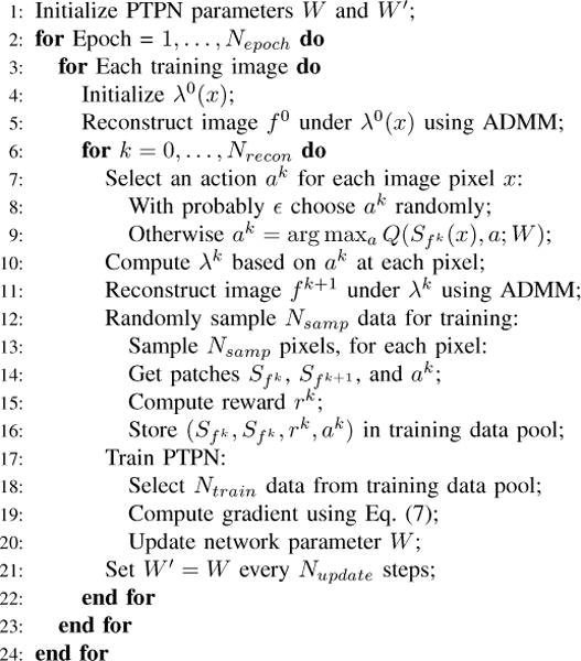
Overall algorithm used to train the PTPN.

D. Implementation details

We implement this algorithm using Python with Tensor-Flow. The computational platform is a desktop workstation with an Intel Xeon 3.5 GHz CPU processor, 8 GB memory and an Nvidia Quadro M4000 GPU card.

For the CT reconstruction part, we consider a fan-beam projection geometry with 180 projections equally spaced over a 2π angular range. The image has a resolution of 128 × 128 pixels. A relatively low resolution is used in this study due to computational efficiency concerns. The x-ray detector is of a line shape with 384 elements covering a 40 cm range. The source-to-isocenter distance is 100 cm and the isocenter-to-detector distance is 50 cm. The projection matrix P is computed using the standard Siddon’s algorithm [33]. We select six slices of CT images at different anatomical sites including brain, lung, and abdomen from different patients as training images and another six slices of CT images as testing samples, see Fig. 4. Note that although only six CT slices are used, the actual number of training pairs is substantially larger in the deep-reinforcement learning scheme, as indicated in Table I. Projection data is simply calculated as g = P f^∗+n, where f^∗ is the ground truth image and n is a Gaussian noise signal with zero mean and variance determined by P f^∗ as in a previous study [34]. The averaged relative noise level is 3%. Values of relevant parameters used in training are summarized in Table I.

Fig. 4.

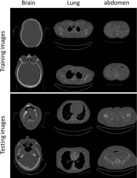
Training (top) and testing images (buttom) used in this study.

TABLE I.

Relevant parameters used, when training the PTPN.

Parameter	Value	Comments
δ	3 × 10−3	Stopping criteria in ADMM
γ	0.99	Discount rate
ε	0.99 ∼ 0.1	Parameter of ε-greedy approach
Nepoch	100	Number of epochs
Nsamp	3200	Number of sampled patches to add to training data pool
Nrecon	20	Number of times to perform ADMM reconstruction per epoch
σ	0.001	Learning rate when updating W
Ntrain	128	Number of data for training each time
Nupdate	300	Number of steps to update W′ = W

III. Validation studies and results

A. Training process and trained PTPN

During the training process, we monitor the quality of the trained PTPN, as shown in Fig. 5. Both the average output of the PTPN and the reward follow an increasing trend, albeit with some oscillations. This indicates that the PTPN is adjusted gradually in this reinforcement learning process towards predicting actions with high reward values. We remark here that the overall training time is around 20 hours under the current setup.

Fig. 5.

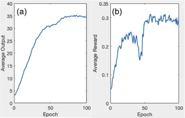
Average output of PTPN (a) and reward (b) in each training epoch.

B. Parameter tuning in CT reconstruction

1) CT reconstruction under PTPN guidance

With the PTPN trained, we use it to guide parameter tuning in a CT reconstruction problem. As such, we select a ground truth CT image f^∗ and generate the projection data with noise added. We first set the parameter arbitrarily to λ⁰(x) = 0.005, a constant value that is likely not optimal. After that, we apply PTPN to guide parameter tuning as outlined in the beginning of Sec.II.B. The tuning process stops, when the relative difference between CT images in two successive reconstructed images is less than 1%.

To observe this process in detail, we select a test case that is not used in training. Fig. 6(a)-(c) present reconstructed CT images at steps k = 1, 4, 7. It is clear that the image quality is improved with the parameter tuned. Quantitatively, we compute the relative error e = |f − f^∗|/|f^∗| at different steps and plot it in Fig. 6(d). A monotonic decay trend is observed, indicating the effectiveness of parameter tuning. Note that a single reconstruction process in the current setup takes around 7 seconds. In the proposed scheme, we have restricted the number of parameter-tuning steps to be no larger than 20. Therefore, the maximum computational time for a complete parameter tuning and reconstruction process is approximately 140 seconds. In practice, the running time should always be shorter, since the reconstructed image from one step is utilized as the initial guess of the next step, which promises a fast convergence. In all the testing cases, we observed that the parameter-tuning processes often stop after 7-12 steps with less than 60 seconds of overall running time.

Fig. 6.

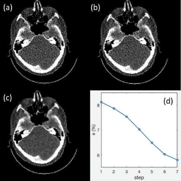
(a)-(c) Reconstructed images at step 1, 4, and 7. CT images are displayed in the window [−100, 300] HU. (d) Error e(%) as a function of parameter-tuning step.

2) Reconstruction results

Fig. 7 is a case that is used in training, whereas Fig. 8 is the same case shown in Fig. 6, which is not included in training. Since we arbitrarily set initial values of λ(x), which is too small in these two cases, the resulting images contain a lot of noise (Fig. 7(b) and 8(b)). After the parameter λ(x) is tuned by PTPN, the image quality in both cases is substantially improved (Fig. 7(c) and 8(c)).

Fig. 7.

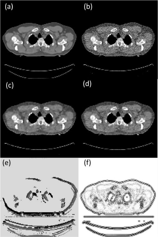
(a) Ground truth CT image of a case that is used in training PTPN. (b) Image reconstructed with an arbitrarily selected parameter λ(x) = 0.005. (c) Image reconstructed after the parameter is tuned by PTPN. (d) Image reconstructed with manually tuned λ(x) = 0.05. CT images are displayed in the window [−100, 300] HU. (e) Tuned parameter map λ(x) displayed in log₁₀ scale. (f) Optimal parameter map λ^∗(x).

Fig. 8.

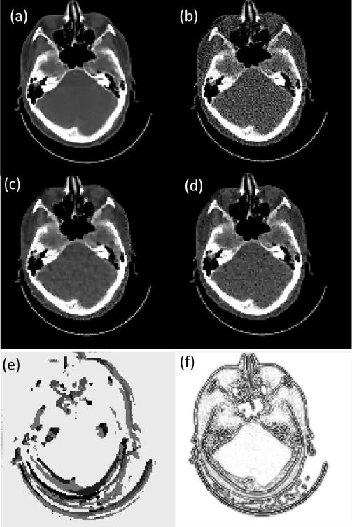
(a) Ground truth CT image of a case that is not used in training PTPN. (b) Image reconstructed with an arbitrarily selected parameter λ(x) = 0.005. (c) Image reconstructed after the parameter is tuned by PTPN. (d) Image reconstructed with manually tuned λ(x) = 0.12. CT images are displayed in a window [−100, 300] HU. (e) Tuned parameter map λ(x) displayed in log₁₀ scale. (f) Optimal parameter map λ^∗(x).

We compare the results with those under manually tuned parameters. Since it is impractical for one to adjust the parameter for each individual pixel, we consider a special context that the parameter is a constant throughout the image and we manually adjust this parameter value for the best image quality. The appropriate parameter values are λ(x) = 0.05 for Fig. 7 and λ(x) = 0.12 for Fig. 8. Fig. 7(d) and 8(d) depict images reconstructed under these parameters in the two cases, respectively. It is found that the images still contain a certain amount of noise and the quality is inferior to those reconstructed with parameters tuned by PTPN.

As for the parameter maps tuned by the PTPN shown in Fig. 7(e) and 8(e), it is observed that PTPN deliberately reduces parameter values around image edges. This is understandable. Reducing parameters at those pixels decreases the strengths of regularization in those areas, which is beneficial in terms of preserving image edges.

Interestingly, for the simple problem in Eq. (2), it is possible to derive the optimal parameter map λ^∗(x). As such, let us take the gradient of the objective function and set it to zero at $f=f^{\ast }:P^T(Pf-g)-\mathrm{\lambda }\nabla \cdot {\left(\frac{\nabla f}{\left|\nabla f\right|}\right)|}_{f=f^{\ast }}=0$. This implies that the optimal parameter map is

$${\mathrm{\lambda }}^{\ast }(x)=\frac{P^T(P{f}^{\ast }-g)}{\nabla \cdot \left(\frac{\nabla f^{\ast }}{\left|\nabla f^{\ast }\right|}\right)}.$$ (9)

The numerator in this expression is more or less an image of noise that is obtained by back-projecting the residual error in the projection domain to the image domain. Here, we neglect the image structure of the noise and plot the image $1/\nabla \cdot \left(\frac{\nabla f^{\ast }}{\left|\nabla f^{\ast }\right|}\right)$ in Fig. 7(f) and 8(f) for the two cases, respectively. The images shows that λ^∗(x) is small along the image edges. Comparing subfigures (e) and (f) in Fig. 7 and Fig. 8, the similarity between corresponding pair of images implies that PTPN can intelligently adjust λ(x) towards the optimal parameter maps. Note that this intelligence is purely developed by the PTPN itself through the reinforcement learning process. Except for providing rewards for an action, we do not explicitly give any information regarding how to tune the parameters.

Quantitatively, we evaluate the image quality using relative error e and Peak Signal-to-Noise Ratio (PSNR). Table II summarizes the results in the six training and the six testing cases. In each case, we present the metrics for the images under a manually tuned parameter, under an arbitrarily set initial parameters, and under parameters tuned by PTPN. For all the training cases, the images under PTPN-tuned parameters achieve the smallest errors and the highest PSNRs, indicating effectiveness of PTPN. Among the six testing cases, the PTPN-tuned parameters yield the smallest errors and the highest PSNRs in five cases (#1-4, 6). For the case #5, the difference between the manually tuned and the PTPN-tuned results is small.

TABLE II.

Relative error and PSNR OF IMAGE RECONSTRUCTION RESULTS. BOLDFACE NUMBERS INDICATE THE BEST RESULT IN EACH CASE.

Case		eManual(%)	eInitial(%)	eTuned(%)	PSNRManual(dB)	PSNRInitial(dB)	PSNRTuned(dB)
Training	1	4.47	7.50	4.21	39.13	34.65	39.67
	2	4.69	7.72	4.56	38.67	34.33	38.90
	3	10.77	11.89	10.38	31.57	30.70	31.89
	4	12.92	13.61	12.54	29.56	29.11	29.82
	5	3.68	6.83	3.62	40.04	35.07	40.59
	6	3.82	6.78	3.55	41.09	36.11	41.74
Testing	1	4.35	6.93	4.24	44.28	40.22	44.50
	2	12.17	12.35	12.13	29.45	29.32	29.48
	3	10.30	11.49	8.48	32.14	31.19	33.83
	4	5.42	8.17	5.32	36.67	33.10	36.89
	5	4.62	7.19	4.95	36.91	33.07	36.31
	6	8.56	10.29	7.56	31.69	30.09	32.78

3) Application to other cases

PTPN determines the way of parameter tuning based on observed image patch. It is expected that the trained PTPN is also applicable to image reconstruction problems under settings that are different from those in training. To demonstrate this fact, we also apply PTPN to CT reconstruction in cases with different number of projections, noise levels, projection geometry, as well as a real phantom case. Fig. 9(a) and (b) use the same CT image as in Fig. 8 but with 2% and 5% noise in the projection data, different from the noise level of 3% in training. Fig. 9(c) is the case with only 90 projections. In Fig. 9(d) we change the isocenter-to-detector distance to 25 cm. In all the cases, PTPN is able to adjust parameters to yield images with satisfactory quality. The resulting parameter maps in Fig. 9(e)-(h) are all similar to the ground truth shown in Fig. 8(f).

Fig. 9.

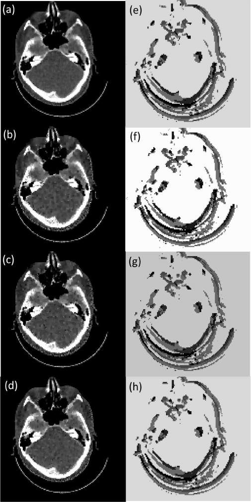
(a)-(b) The results under tuned parameter for a case with 2% and 5% noise in the projection data. (c) The result with 90 projections. (d) The result with isocenter-to-detector distance changed to 25 cm. CT images are displayed in the window [−100, 300] HU. Figures in the right column are tuned parameter maps displayed in log₁₀ scale for corresponding figures in the left column.

In Fig. 10, we report the result generated by applying the trained PTPN to a real phantom case. A Catphan 504 phantom is scanned on a Cone beam CT of a Varian TrueBeam medical linear accelerator (Varian Medical System. Palo Alto, CA) using 100 kVp and 0.4 mAs. The x-ray is collimated to a 2 cm thick fan beam to reduce scatter. Only the central CT slice is reconstructed. It can be observed that PTPN leads to better image quality than results using the initial parameter and the manually tuned parameter.

Fig. 10.

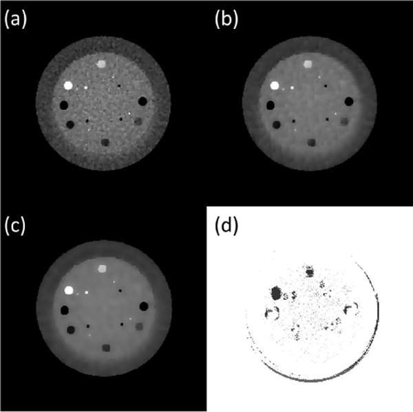
Image reconstructed with an arbitrarily selected parameter λ(x) = 0.005. (b) Image reconstructed by manually tuned to λ(x) = 0.15. (c) Image reconstructed after the parameter is tuned by PTPN. CT images are displayed in the windows [−200, 500] HU. (d) Tuned parameter map λ(x) displayed in log₁₀.

IV. Discussions

Relation to other works

The power of deep learning in medical image processing has been clearly demonstrated in a spectrum of problems. Among these studies, most used supervised learning to determine parameters inside a network in order to establish a map between input and output images. In [22], [23], a network was set up to map a noise-contaminated CT image acquired at a low-dose level to the clean image. In [19], deep residual learning was employed to map a CT image with streak artifacts caused by undersampling to the artifact image, which was further subtracted from the original image to eliminate the artifact. In a study [35] that viewed the iterative image reconstruction process as a data flow in a network under the ADMM algorithm, the supervised learning process enabled discovery of the algorithm parameters, such as image filters and threshold values. Comparing to these novel works, our study is different in two-fold. First, the purpose of using deep learning is different. Instead of trying to predict the underlying true solution or image artifacts, the purpose of setting up a PTPN is to predict a dynamic policy applicable to the image reconstruction problem in Eq. (2). Under the guidance of this policy, the output image of the reconstruction algorithm is directed towards a satisfactory quality. Second, the method to train our network is also different from the supervised training in previous works. Instead of using labeled training pairs in a supervised training fashion, we employed the reinforcement learning strategy. This strategy let the algorithm make its own decisions and obtain rewards based on the image and the selected action. Through the training process, the PTPN spontaneously discovered the appropriate strategy for an input system state. This was the process in which intelligence was generated.

The CT reconstruction problem with pixel-wise regularization has been investigated in previous studies [9], [10]. It was proposed to perform a sequence of reconstructions with parameters adjusted based on the reconstructed images. The motivation was to detect image edges and to tune down the regularization strengths for the purpose of edge preservation. As opposed to designing an explicit rule of parameter tuning, this study discovered the rule via the reinforcement learning process. It is interesting to observe that intelligence can be correctly generated, which coincides with previous human knowledge.

Necessity of deep reinforcement learning

What is ultimately learned by PTPN is evaluation of the image quality and the link to parameter tuning. With this in mind, one may argue that the complex reinforcement learning technique is probably unnecessary, as one can simply perform supervised learning by using a sizable data set containing paired data of image patches and corresponding ways of parameter tuning. We agree with this statement to a certain extent, but still think our study is meaningful. For this CT reconstruction problem, it is straightforward to generate labeled training pairs (image patch and direction of parameter tuning) to allow supervised training. Yet if we would like to label an image patch with not only the direction of parameter tuning, i.e. increase or decrease, but also with the amount of parameter change, i.e. 50% or 20% as in our example, it becomes quite difficult to generate training data. Hence, the advantage of reinforcement learning is to automatically learn a more comprehensive policy. Beyond the problem of CT reconstruction, it may not be easy to generate labeled training pairs in many optimization-based inverse problems. However, since very often one has a good sense of judging the output results, it is still relatively easy to quantify the result quality change via a reward function. This allows the use of reinforcement learning to establish the policy in those problems for which labeled training pairs are hard to get.

Relevance to other problems

This study uses an optimization-based iterative CT reconstruction problem as an example to show that it is possible to achieve intelligent parameter tuning via a deep learning framework. With the rapid growth of deep learning techniques in CT reconstruction area, the impact of this study may diminish. However, we think studying the general task of parameter tuning is still of significance and deep learning opens a new window to tackle this problem. First, parameter tuning is not a problem unique to the CT reconstruction regime, but generally exists in many areas. Even beyond the scope of image processing, many other decision making problems in medicine can be solved via an optimization approach, for which parameter tuning is an indispensable task. One notable example is treatment planning in cancer radiation therapy [36]. Even with a modern treatment planning system to solve the underlying optimization problem, a hospital still needs to hire a number of dosimetrists to manually tune the parameters in order to generate plans meeting clinician’s requirements. This fact clearly highlights the need for and potential benefits of an intelligent parameter-tuning system. Second, even for the deep learning technique itself, the training stage has a number of parameters to be tuned by the researchers to achieve the best performance. These parameters include, but are not limited to, learning rate, number of epochs, size and number of filters, etc. It would be an interesting and important step to develop a parameter-tuning system to handle the adjustment of these parameters. Meanwhile, we have to admit that solving the parameter-tuning problem in the area beyond the simple example of CT reconstruction is apparently much more challenging. We hope our study can shed some light in this direction and trigger deeper investigations in future.

Limitations and future directions

This study has the following limitations. First, due to the limitation on computational power, we only considered images with a relatively low resolution in a small number of cases. It is our plan to extend the studies to high-resolution images that are of more clinical relevance. We will also use more cases for training and testing to yield a more robust PTPN. The second limitation of this study is that PTPN has to wait for the ADMM iterative process to finish, before it can adjust parameters. Although the image quality resulting from this this approach is acceptable, waiting for the ADMM iteration to finish reduces the overall workflow efficiency. This can be potentially improved by using another reconstruction algorithm with a higher convergence rate. Another possible way of acceleration is to predict the converged CT image at an early stage of the ADMM iteration, for instance using a deep learning approach [24]. Third, PTPN lays a general framework on the development of a strategy to improve image quality. The current setup in Eq. (2) limits the possible choices of parameter change to five options. However, in general, it is possible to include options that more directly affect the images, such as actions to reduce noise and artifacts, etc. It is noted that deep-learning has achieved tremendously in each of these CT image enhancement approaches [19]–[21]. Using them under the guidance of a policy network is expected to yield a comprehensive image reconstruction system that can automatically handle various of data contaminations. Last, but no the least, in several studies the optimal parameter values for the reconstruction problem are indeed known based on physics models [16] or mathematical analysis [17]. It will be an interesting future study to extend the proposed method to these contexts and compare the PTPN-tuned parameters with the theoretically predicted optimal values. This will offer the opportunity to assess the proposed method in an objective manner.

V. Conclusion

In this paper, we presented a novel method for automatic parameter tuning in an optimization problem, which is a typical task in a number of image-processing, or non-image-processing problems. The significance of this study is underscored by the fact that the solution quality is critically determined by the parameter values, and yet there is no satisfactory way of automatically adjusting parameters. We proposed to solve this problem by constructing a policy network, which can be trained to guide parameter tuning. We demonstrated our idea in an example problem of optimization-based iterative CT reconstruction with a pixel-wise TV regularization term. We configured a PTPN to map a CT image patch to the direction and magnitude of tuning the parameter at the patch center. PTPN was trained via an end-to-end reinforcement learning procedure. A series tests demonstrated that the trained PTPN is able to intelligently determine the way of parameter adjustment. Under the guidance of PTPN, the reconstructed CT images achieved image quality similar or better than that under manually tuned parameters.

References

- 1.Rudin LI, Osher S, Fatemi E. Nonlinear total variation based noise removal algorithms. Physica D: Nonlinear Phenomena. 1992;60(1):259–268. [Online]. Available: http://www.sciencedirect.com/science/article/pii/016727899290242F. [Google Scholar]
- 2.Sidky EY, Pan X. Image reconstruction in circular cone-beam computed tomography by constrained, total-variation minimization. Physics in Medicine and Biology. 2008;53(17):4777. doi: 10.1088/0031-9155/53/17/021. [Online]. Available: http://stacks.iop.org/0031-9155/53/i=17/a=021. [DOI] [PMC free article] [PubMed] [Google Scholar]
- 3.Jia X, Lou Y, Li R, Song WY, Jiang SB. Gpu-based fast cone beam ct reconstruction from undersampled and noisy projection data via total variation. Medical Physics. 2010;37(4):1757–1760. doi: 10.1118/1.3371691. [Online]. Available: http://dx.doi.org/10.1118/1.3371691. [DOI] [PubMed] [Google Scholar]
- 4.Dong B, Shen Z, Series M, Dong B, Shen Z, Dong B, Shen Z. Mra-based wavelet frames and applications in IAS Lecture Notes Series, Summer Program on The Mathematics of Image Processing. Park City Mathematics Institute; 2010. [Google Scholar]
- 5.Jia X, Dong B, Lou Y, Jiang SB. Gpu-based iterative cone-beam ct reconstruction using tight frame regularization. Physics in Medicine and Biology. 2011;56(13):3787. doi: 10.1088/0031-9155/56/13/004. [Online]. Available: http://stacks.iop.org/0031-9155/56/i=13/a=004. [DOI] [PubMed] [Google Scholar]
- 6.Lou Y, Zhang X, Osher S, Bertozzi A. Image recovery via nonlocal operators. Journal of Scientific Computing. 2010 Feb;42(2):185–197. [Online]. Available: https://doi.org/10.1007/s10915-009-9320-2. [Google Scholar]
- 7.Chen Z, Qi H, Wu S, Xu Y, Zhou L. Few-view ct reconstruction via a novel non-local means algorithm. Physica Medica. 2016;32(10):1276–1283. doi: 10.1016/j.ejmp.2016.05.063. [Online]. Available: http://www.sciencedirect.com/science/article/pii/S1120179716301077. [DOI] [PubMed] [Google Scholar]
- 8.Jia X, Tian Z, Lou Y, Sonke J-J, Jiang SB. Four-dimensional cone beam ct reconstruction and enhancement using a temporal nonlocal means method. Medical Physics. 2012;39(9):5592–5602. doi: 10.1118/1.4745559. [Online]. Available: http://dx.doi.org/10.1118/1.4745559. [DOI] [PMC free article] [PubMed] [Google Scholar]
- 9.Guo W, Yin W. Edgecs: edge guided compressive sensing reconstruction. Proc SPIE. 2010;7744:7744–7744. 10. [Online]. Available: http://dx.doi.org/10.1117/12.863354. [Google Scholar]
- 10.Tian Z, Jia X, Yuan K, Pan T, Jiang SB. Low-dose ct reconstruction via edge-preserving total variation regularization. Physics in Medicine and Biology. 2011;56(18):5949. doi: 10.1088/0031-9155/56/18/011. [Online]. Available: http://stacks.iop.org/0031-9155/56/i=18/a=011. [DOI] [PMC free article] [PubMed] [Google Scholar]
- 11.Golub GH, Heath M, Wahba G. Generalized cross-validation as a method for choosing a good ridge parameter. Technometrics. 1979;21(2):215–223. [Online]. Available: http://www.jstor.org/stable/1268518. [Google Scholar]
- 12.Hansen PC. Analysis of discrete ill-posed problems by means of the l-curve. SIAM Review. 1992;34(4):561–580. [Online]. Available: https://doi.org/10.1137/1034115. [Google Scholar]
- 13.Ramani S, Liu Z, Rosen J, Nielsen JF, Fessler JA. Regularization parameter selection for nonlinear iterative image restoration and mri reconstruction using gcv and sure-based methods. IEEE Transactions on Image Processing. 2012 Aug;21(8):3659–3672. doi: 10.1109/TIP.2012.2195015. [DOI] [PMC free article] [PubMed] [Google Scholar]
- 14.Zhu X, Milanfar P. Automatic parameter selection for denoising algorithms using a no-reference measure of image content. IEEE Transactions on Image Processing. 2010 Dec;19(12):3116–3132. doi: 10.1109/TIP.2010.2052820. [DOI] [PubMed] [Google Scholar]
- 15.Liang H, Weller DS. Comparison-based image quality assessment for selecting image restoration parameters. IEEE Transactions on Image Processing. 2016 Nov;25(11):5118–5130. doi: 10.1109/TIP.2016.2601783. [DOI] [PubMed] [Google Scholar]
- 16.Bai T, Yan H, Ouyang L, Staub D, Wang J, Jia X, Jiang SB, Mou X. Data correlation based noise level estimation for cone beam projection data. Journal of X-Ray Science and Technology, no Preprint. 2017:1–20. doi: 10.3233/XST-17266. [DOI] [PMC free article] [PubMed] [Google Scholar]
- 17.Zhang H, Dang H, Gang GJ, Stayman JW. Prospective regularization analysis and design for prior-image-based reconstruction of x-ray ct. in Proceedings of the International Meeting on Fully Three-Dimensional Image Reconstruction in Radiology and Nuclear Medicine. 2017;14:417–23. [Google Scholar]
- 18.Wang G. A perspective on deep imaging. IEEE Access. 2016;4:8914–8924. [Google Scholar]
- 19.Han Y, Yoo JJ, Ye JC. Deep residual learning for compressed sensing CT reconstruction via persistent homology analysis. CoRR. 2016 abs/1611.06391. [Online]. Available: http://arxiv.org/abs/1611.06391.
- 20.Kang E, Min J, Ye JC. Wavenet: a deep convolutional neural network using directional wavelets for low-dose x-ray CT reconstruction. CoRR. 2016 doi: 10.1002/mp.12344. abs/1610.09736. [Online]. Available: http://arxiv.org/abs/1610.09736. [DOI] [PubMed]
- 21.Li H, Mueller K. Low-dose ct streak artifacts removal using deep residual neural network. Proceedings of Fully 3D conference 2017. 2017:191–194. [Google Scholar]
- 22.Chen H, Zhang Y, Zhang W, Liao P, Li K, Zhou J, Wang G. Low-dose ct via convolutional neural network. Biomed Opt Express. 2017 Feb;8(2):679–694. doi: 10.1364/BOE.8.000679. [Online]. Available: http://www.osapublishing.org/boe/abstract.cfm?URI=boe-8-2-679. [DOI] [PMC free article] [PubMed] [Google Scholar]
- 23.Chen H, Zhang Y, Kalra MK, Lin F, Chen Y, Liao P, Zhou J, Wang G. Low-dose ct with a residual encoder-decoder convolutional neural network (red-cnn) IEEE Transactions on Medical Imaging. 2017;(99):1–1. doi: 10.1109/TMI.2017.2715284. PP. [DOI] [PMC free article] [PubMed] [Google Scholar]
- 24.Cheng L, Ahn S, Ross S, Qian H, Man BD. Accelerated iterative image reconstruction using a deep learning based leapfrogging strategy. Proceedings of Fully 3D conference 2017. 2017:715–720. [Google Scholar]
- 25.Mnih V, Kavukcuoglu K, Silver D, Graves A, Antonoglou I, Wierstra D, Riedmiller MA. Playing atari with deep reinforcement learning. CoRR. 2013 abs/1312.5602. [Online]. Available: http://arxiv.org/abs/1312.5602.
- 26.Mnih V, Kavukcuoglu K, Silver D, Rusu AA, Veness J, Bellemare MG, Graves A, Riedmiller M, Fidjeland AK, Ostrovski G, et al. Human-level control through deep reinforcement learning. Nature. 2015;518(7540):529–533. doi: 10.1038/nature14236. [DOI] [PubMed] [Google Scholar]
- 27.Goldstein T, Osher S. The split bregman method for l1-regularized problems. SIAM Journal on Imaging Sciences. 2009;2(2):323–343. [Online]. Available: https://doi.org/10.1137/080725891. [Google Scholar]
- 28.Chambolle A, Pock T. A first-order primal-dual algorithm for convex problems with applications to imaging. Journal of Mathematical Imaging and Vision. 2011 May;40(1):120–145. [Online]. Available: https://doi.org/10.1007/s10851-010-0251-1. [Google Scholar]
- 29.Boyd S, Parikh N, Chu E, Peleato B, Eckstein J. Distributed optimization and statistical learning via the alternating direction method of multipliers. Found Trends Mach Learn. 2011 Jan;3(1):1–122. [Online]. Available: http://dx.doi.org/10.1561/2200000016. [Google Scholar]
- 30.Golub G, Van Loan C. Matrix Computations, ser. Johns Hopkins Studies in the Mathematical Sciences. Johns Hopkins University Press; 2013. [Online]. Available: https://books.google.com/books?id=X5YfsuCWpxMC. [Google Scholar]
- 31.Watkins CJCH, Dayan P. Q-learning. Machine Learning. 1992 May;8(3):279–292. [Online]. Available: https://doi.org/10.1007/BF00992698. [Google Scholar]
- 32.Bellman R, Karush R. ser. Memorandum (Rand Corporation) Rand Corporation; 1964. Dynamic Programming: A Bibliography of Theory and Application. [Online]. Available: https://books.google.com/books?id=zHG1AQAACAAJ. [Google Scholar]
- 33.Siddon RL. Fast calculation of the exact radiological path for a three-dimensional ct array. Medical Physics. 1985;12(2):252–255. doi: 10.1118/1.595715. [Online]. Available: http://dx.doi.org/10.1118/1.595715. [DOI] [PubMed] [Google Scholar]
- 34.Wang J, Lu H, Liang Z, Eremina D, Zhang G, Wang S, Chen J, Manzione J. An experimental study on the noise properties of x-ray ct sinogram data in radon space. Physics in Medicine and Biology. 2008;53(12):3327. doi: 10.1088/0031-9155/53/12/018. [Online]. Available: http://stacks.iop.org/0031-9155/53/i=12/a=018. [DOI] [PMC free article] [PubMed] [Google Scholar]
- 35.Yang Y, Sun J, Li H, Xu Z. Deep admm-net for compressive sensing mri. In: Lee DD, Sugiyama M, Luxburg UV, Guyon I, Garnett R, editors. Advances in Neural Information Processing Systems. Vol. 29. Curran Associates, Inc; 2016. pp. 10–18. [Online]. Available: http://papers.nips.cc/paper/6406-deep-admm-net-for-compressive-sensing-mri.pdf. [Google Scholar]
- 36.Bortfeld T. Imrt: a review and preview. Physics in medicine and biology. 2006;51(13):R363. doi: 10.1088/0031-9155/51/13/R21. [DOI] [PubMed] [Google Scholar]