A Fast Algorithm for Convolutional Structured Low-rank Matrix Recovery

Abstract

Fourier domain structured low-rank matrix priors are emerging as powerful alternatives to traditional image recovery methods such as total variation (TV) and wavelet regularization. These priors specify that a convolutional structured matrix, i.e., Toeplitz, Hankel, or their multi-level generalizations, built from Fourier data of the image should be low-rank. The main challenge in applying these schemes to large-scale problems is the computational complexity and memory demand resulting from a lifting the image data to a large scale matrix. We introduce a fast and memory efficient approach called the Generic Iterative Reweighted Annihilation Filter (GIRAF) algorithm that exploits the convolutional structure of the lifted matrix to work in the original un-lifted domain, thus considerably reducing the complexity. Our experiments on the recovery of images from undersampled Fourier measurements show that the resulting algorithm is considerably faster than previously proposed algorithms, and can accommodate much larger problem sizes than previously studied.

I. Introduction

Recovering image data from limited and noisy measurements is a central problem in many biomedical imaging problems, including MRI, microscopy, and tomography. The conventional approach to solve these ill-posed problems is to regularize the recovery using smoothness or sparsity priors in discrete image domain, as in compressed sensing-based MRI reconstruction [1]. In contrast to this approach, several researchers have proposed a new class of recovery algorithms that impose a low-rank penalty on a convolutional structured matrix constructed from Fourier data of the image, i.e., a matrix that is Toeplitz, Hankel, or their multi-level generalizations [2]–[8]. These convolutional structured low-rank matrix penalties are emerging as powerful alternatives to conventional discrete spatial domain penalties because of their ability to exploit continuous domain analogs of sparsity. These methods are often called “off-the-grid”, in the sense that they do not require discrete gridding of the signal in spatial domain. This is because these methods model linear dependencies among the Fourier coefficients of the image induced by low-complexity continuous domain properties of the image (detailed below). In particular, the linear dependencies can be expressed as a nulling of the Fourier coefficients of the image by convolution with a finite impulse response filter—a so-called “annihilation relationship”—that translates directly to the low-rank property of a Toeplitz-like matrix built from the Fourier coefficients. These methods then pose image recovery either partially or entirely in Fourier domain as a structured low-rank matrix recovery problem, where the structure of the matrix encodes the particular modeling assumptions.

The linear dependencies between the Fourier coefficients exploited the in structured low-rank matrix priors result from a variety of assumptions, including continuous domain analogs of sparsity [3], [6], [8], [9], correlations in the locations of the sparse coefficients in space [8], [9], multi-channel sampling [2], [10], [11], or smoothly varying complex phase [4]. For example, the LORAKS framework [4] capitalized on the sparsity and smooth phase of the continuous domain image using structured low-rank priors, which offers improved reconstructions over conventional ℓ₁ recovery. Similarly, we have shown that the Fourier coefficients of continuous domain piecewise constant images whose discontinuities are localized to zero level-set of a bandlimited function satisfy an annihilation relationship [9]; their recovery from undersampled Fourier measurements translates to a convolutional structured low-rank matrix completion problem [8]. This model, which exploits the smooth structure of the discontinuities along with sparsity, can lead to significant improvement in reconstruction quality over traditional methods such as total variation (TV) minimization; see [8], [9] for more details. Similarly, the ALOHA framework [6] reformulates the recovery of a transform sparse signal as a structured low-rank matrix recovery problem, e.g., images that are sparse under the undecimated Harr wavelet transform. Inspired by auto-calibration techniques in parallel MRI [12]–[15], the extension to recovery of parallel MRI from undersampled measurements is formulated as a structured low-rank matrix recovery problem in [2], [10]. Similar approaches have also been found very effective in auto-calibrated multishot MRI [16] and correction of echo-planar MRI data [17]. The theoretical performance of structured low-rank matrix completion methods has been studied in [3], [18], [19], showing improved statistical performance over standard discrete spatial domain recovery.

Despite improvements in empirical and statistical recovery performance over traditional methods as seen from [2]–[4], [6], [8], [16], these structured low-rank matrix recovery schemes are associated with a dramatic increase in computational complexity and memory demand; this restricts their direct extension to multi-dimensional imaging applications, such as dynamic MRI reconstruction. In particular, these algorithms involve the recovery of a large-scale Toeplitz-like matrix whose combined dimensions are several orders of magnitude larger than those of the image. For example, the dimension of the structured matrix is roughly 10⁶ ×2000 for a realistic scale 2-D MRI reconstruction problem (see Table I), while the matrix is several orders of magnitude larger in dynamic MRI applications, making it impossible to store. Moreover, typical algorithms require a singular value decomposition (SVD) of the dense large-scale matrix at each iteration, which is computationally prohibitive for large-scale problems. Several strategies have been introduced to minimize or avoid SVD’s in these algorithms. For example, the algorithms derived in [4], [6] replace the full SVD’s with more efficient truncated SVD’s or matrix inversions by assuming the matrix to be recovered is low-rank, or well approximated as such. However, even with these low-rank modifications, the algorithms in [4], [6] still have considerable memory demand, since they require storing a variable having dimensions of the large-scale matrix.

TABLE I.

Convergence time of algorithms for structured low-rank recovery of piecewise constant images from noise-free random fourier samples.

Problem					AP		SVT		SVT+UV		IRLS-0		GIRAF-0
dataset	data size	filter	rank	USF	# iter	time (s)	# iter	time (s)	# iter	time (s)	# iter	time (s)	# iter	time (s)
PWC1	65×65	9×9	32	0.50	17	5.4	11	1.1	11	0.8	3	17.5	3	0.6
PWC1	65×65	9×9	32	0.33	39	12.8	–	Inf	19	1.4	4	24.5	5	1.4
PWC2	129×129	17×17	118	0.50	19	48.0	9	25.2	15	21.6	4	566.6	3	1.1
PWC2	129×129	17×17	118	0.33	90	228.0	–	Inf	24	36.2	7	1032.8	5	2.6
SL	201×201	25×25	336	0.65	31	762.0	13	338.7	11	150.9	–	Mem	3	3.7
SL	201×201	25×25	336	0.50	88	2151.7	–	Inf	36	494.4	–	Mem	4	4.7
BRAIN	255×255	45×45	1250	0.65	–	Mem	–	Mem	23	4270.3	–	Mem	3	25.2
BRAIN	255×255	45×45	1250	0.50	–	Mem	–	Mem	–	Inf	–	Mem	5	55.3

Stopping criteria: NMSE ≤ 10⁻⁴.

Key: Inf - Algorithm converged above NMSE threshold. Mem - Not enough memory to run algorithm.

Computer specifications: Intel Xeon 3.20GHz CPU and 24 GB RAM.

In this paper we introduce a novel, fast algorithm for a class of convolutional structured low-rank matrix recovery problems arising in MRI reconstruction and other imaging contexts. What distinguishes the algorithm from other approaches is its direct exploitation of the convolutional structure of the matrix—none of the current algorithms fully exploit this structure. This enables us to evaluate the intermediate steps of the algorithm efficiently using fast Fourier transforms in the original problem domain, resulting in an algorithm with significant reductions in memory demand and computational complexity. Our approach does not require storing or performing computations on the large-scale structured matrix, nor do we need to make overly strict low-rank assumptions about the solution. The proposed approach is based on the iterative reweighted least squares (IRLS) algorithm for low-rank matrix completion [20]–[22], which we adapt to the convolutional structured matrix setting. This algorithm minimizes the nuclear norm or the non-convex Schatten-p quasi-norm of the structured matrix subject to data constraints. However, as we show, the direct extension of the IRLS algorithm to the large-scale setting does not yield a fast algorithm. We additionally propose a systematic approximation of convolutional structured matrices that radically simplifies the subproblems of the IRLS algorithm, while keeping the low-rank property of the matrix intact. The combination of these two ingredients, the IRLS algorithm and the proposed approximation of the convolutional structured matrices, we call the generalized iterative reweighted annihilating filter (GIRAF) algorithm. The name reflects the fact that the algorithm can be interpreted as alternating between (1) the robust estimation of an annihilating filter for the data, and (2) solving for the data best annihilated by the filter in a least squares sense.

Finally, we note that several existing approaches for inverse problems in imaging utilize non-convex approaches, similar to the present work. For example, an augmented Lagrangian iterative shrinkage algorithm for non-convex Schatten p-norms has been introduced for the denoising of images in [23]. However, since these schemes apply low-rank denoising on groups of non-local patches, the matrices in their setting are considerably smaller than in our context and does not possess the convolutional structure that we consider in this work. Similarly, the non-convex penalties studied in [24], [25] are discrete formulations using non-convex vector norms in the image domain; these methods cannot exploit the continuous domain properties that are modeled using structured low-rank penalties, and hence will have limited applicability in the context we consider.

II. Signal reconstruction by convolutional structured low-rank matrix recovery

A. Convolutional structured low-rank matrix models in imaging

Structured low-rank matrix approximation (SLRA) models are widely used in many branches of signal processing [26], [27]. A SLRA model assumes some property of the signal data is equivalent to the low-rank property of a matrix constructed from the data. This paper is motivated by recent convolutional SLRA models in MRI reconstruction [2], [4]–[8], [28], and related inverse problems in imaging [6], [29], [30]. In this setting, various spatial domain properties of the image (e.g., limited support, smooth phase, piecewise constant, etc.) translate into the low-rank property of a convolutional structured matrix (e.g., Toeplitz, Hankel, and their multi-level generalizations) constructed from the Fourier coefficients of the image. Recovery of the image from undersampled or corrupted measurements is then posed in Fourier domain as a convolutional structured low-rank matrix recovery problem.

As a motivating example for the SLRA approach in imaging, consider the class of signals consisting of a sparse linear combination of Dirac impulses in 1-D:

$$\rho (x)={\displaystyle \sum _{i=1}^r{c}_i\delta (x-x_i),\text{for}\text{all}x\in [0,1]}$$ (1)

This signal model is “off-the-grid” in the sense that the impulse locations ${\left\{x_i\right\}}_{i=1}^r$ can be arbitrary points in [0, 1] and are not required to lie on a discrete grid. This example and the analysis that follows is closely related classical methods in line spectral estimation, including Prony’s method [31] and its robust refinements: MUSIC [32], ESPRIT [33], matrix pencil [34], and others. See [35] for a comprehensive overview. These methods utilize the fact that the sparsity of the signal implies a Toeplitz matrix built from the Fourier coefficients of ρ is rank deficient. To see why this is, let μ(x) be a periodic bandlimited function on [0, 1] having r zeros at the Dirac locations ${\left\{x_i\right\}}_{i=1}^r$. It is easily seen that

$$\rho (x)\mu (x)=0\text{for}\text{all}x\in [0,1]$$ (2)

where the equality is understood in the sense of distributions or generalized functions (see, e.g., [36]). This multiplication annihilation relationship in spatial domain translates to a convolution annihilation relationship in Fourier domain:

$$(\widehat{\rho }\ast \widehat{\mu })[k]=0,\text{for}\text{all}k\in \mathbb{Z}$$ (3)

where $\widehat{\rho }$ and $\widehat{\mu }$ denote the Fourier coefficients of ρ and μ. For a finite collection of low-pass Fourier coefficients $\widehat{\rho }[k]$, |k| ≤ K where K is a pre-determined cut-off frequency, the convolution annihilation relationship (3) can be expressed in matrix form as

$$\text{Toep}(\widehat{\rho })\mathit{h}=0.$$ (4)

Here $\text{Toep}(\widehat{\rho })\in {ℂ}^{M\times N}$ denotes a rectangular Toeplitz matrix built from $\widehat{\rho }[k]$, and h ∈ ℂ^N is a vector of the Fourier coefficients of μ, zero-padded if necessary to have length N. This shows h is a non-trivial nullspace vector for $\text{Toep}(\widehat{\rho })$, i.e., $\text{Toep}(\widehat{\rho })$ is rank deficient. Notice also that any multiple of μ(x) by a phase factor, γ(x) = μ(x)e^j2πkx, k ∈ ℤ, will also satisfy the above annihilation relationship, i.e., $\text{Toep}(\widehat{\rho }){\mathit{h}}^{\prime }=0$ where h′ is a vector of the Fourier coefficients of γ. This implies that $\text{Toep}(\widehat{\rho })$ has a large nullspace, hence is a low-rank matrix. In fact, one can show $\text{rank}[\text{Toep}(\widehat{\rho })]=r$, which establishes a one-to-one correspondence between the sparsity of the signal (1) and the rank of a Toeplitz matrix built from its Fourier coefficients.

When we only have samples of $\widehat{\rho }[k]$ for k ∈ Ω where Ω ⊂ ℤ is a sampling set of arbitrary locations, we can use the low-rank property of $\text{Toep}(\widehat{\rho })$ to recover $\widehat{\rho }[k]$ for all |k| ≤ K as the solution to the following matrix completion problem:

$$\underset{\widehat{\varphi }}{min}\text{rank}[\text{Toep}(\widehat{\varphi })]\text{subject to}\widehat{\varphi }[k]=\widehat{\rho }[k],\forall k\in \mathrm{\Omega }$$ (5)

Recovery guarantees for a convex relaxation to (5) were studied in [3] assuming the sampling locations Ω are drawn uniformly at random from the set {k: |k| ≤ K} for some fixed cut-off K. Multi-dimensional generalizations of the model (1) and the recovery program (5) were also considered in [3], and have been adapted to super-resolution imaging context as well [29].

Additionally, SLRA models are central to several MRI reconstruction tasks. An important example is in parallel MRI, where Fourier data of the image is collected simultaneously at multiple receive coils having different spatial sensitivity profiles. Several auto-calibration techniques in parallel MRI, such as GRAPPA [12], ESPIRiT [14], PRUNO [15], and related techniques [13], model the coil sensitivities as smooth functions in spatial domain, which translates to the low-rank property of a convolutional structured matrix built from data obtained at a uniformly sampled calibration region in Fourier domain; see, e.g., [13]. Estimates of the coil sensitivity maps are obtained from the nullspace of this matrix, and then used to reconstruct missing Fourier data via linear prediction. The extension to recovery of parallel MRI without a fully sampled calibration region was formulated as a structured low-rank matrix recovery problem in the SAKE framework [2]. Extensions of this work to the recovery of single coil data was proposed in [4], by modeling the image as having sparse support or smoothly varying phase. This was later incorporated into a multi-coil framework in [10]. Further generalizations of this approach were proposed in [6], which employed transform sparsity of the image, using wavelets and other derivative-like operators.

In the remainder of this paper, we focus on the SLRA model that motivated this work—the continuous domain piecewise smooth image model introduced in [8], [9], [28]. We showed that this class of signals satisfies a Fourier domain convolution annihilation relationship, provided the signal discontinuities are localized to the zero-set of a smooth bandlimited function, as in the finite-rate-of-innovation curves model [37]. This work can also be viewed as an extension of the SLRA models investigated in [38]–[41] in the context of super-resolution MRI, which was formulated for 1-D piecewise polynomial signals. Our work generalizes this model recovery of 2-D piecewise polynomial images with discontinuities supported on curves. For example, suppose f(x, y) is a piecewise constant function in 2-D with discontinuities contained in the zero-set {(x, y) ∈ [0, 1]^2: μ(x, y) = 0} where μ is bandlimited. Analogous to (2), one can show the partial derivatives of f are annihilated by multiplication with μ in spatial domain:

$$({\partial }_{x}f)\mu =0\text{and}({\partial }_{y}f)\mu =0$$ (6)

in the distributional sense; see Figure 1 for an illustration. This translates to the Fourier domain convolution annihilation relationship:

$$(\widehat{{\partial }_{x}f}\ast \widehat{\mu })[k_x,k_y]=0,$$ (7)

$$(\widehat{{\partial }_{y}f}\ast \widehat{\mu })[k_x,k_y]=0\text{for}\text{all}(k_x,k_y)\in {\mathbb{Z}}^2,$$ (8)

Here the expressions $\widehat{{\partial }_{x}f}$ and $\widehat{{\partial }_{y}f}$ are computed in Fourier domain by the weightings

$$\widehat{{\partial }_{x}f}\left[k_x,k_y\right]=j2\pi k_x\widehat{f}[k_x,k_y],$$

$$\widehat{{\partial }_{y}f}\left[k_x,k_y\right]=j2\pi k_y\widehat{f}[k_x,k_y]\text{for}\text{all}(k_x,k_y)\in {\mathbb{Z}}^2,$$

We can represent the convolution relations (7) and (8) in matrix notation as:

$$\mathcal{G}(\widehat{f})\mathit{h}=\left(\begin{array}{c}{\text{Toep}}_2\left(\widehat{{\partial }_{x}f}\right)\\ {\text{Toep}}_2\left(\widehat{{\partial }_{y}f}\right)\end{array}\right)\mathit{h}=0$$ (9)

where ${\text{Toep}}_2(\widehat{g})$ denotes the Toeplitz-like structured matrix built from any 2-D array of coefficients $\widehat{g}$ representing 2-D linear convolution with $\widehat{g}$. Figure 1 illustrates the construction of $\mathcal{G}(\widehat{f})$, which we call the gradient weighted matrix lifting. Similar to the 1-D setting we can show that $\mathcal{G}(\widehat{f})$ is a low-rank matrix. In [9] we proved that under certain geometric restrictions on the edge-set of f, there exists a unique bandlimited annihilating function μ₀ whose shifts in Fourier domain span the nullspace of $\mathcal{G}(\widehat{f})$. In particular, if $\mathcal{G}(\widehat{f})$ is built assuming h ∈ ℂ^N is an array of size Λ ⊂ ℤ², |Λ| = N, then for sufficiently large M one has

$$\text{rank}(\mathcal{G}(\widehat{f}))=N-S,$$ (10)

where S is the number of integer shifts of $\widehat{{\mu }_0}$ inside the index set Λ (see Prop. 6 in [9]). This establishes a correspondence between the rank of $\mathcal{G}(\widehat{f})$ and the complexity of the edge-set of f, as measured by the bandwidth of the annihilating function μ₀.

Fig. 1.

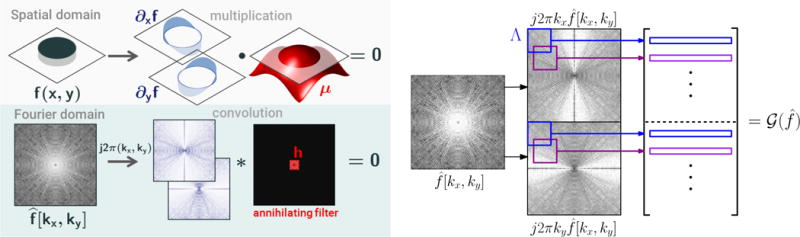
2-D annihilation relationship for piecewise constant images and construction of gradient weighted lifting. If the piecewise constant image f (top) has edges supported in the zero-set of a bandlimited function μ, then the Fourier coefficients of the partial derivatives of f are annihilated by convolution by a filter h determined by the Fourier coefficient of μ. (bottom) From a 2-D array of Fourier coefficients $\widehat{f}$, the matrix $\mathcal{G}(\widehat{f})$ is constructed by weighting $\widehat{f}$ to create two arrays of the simulated Fourier derivatives $\widehat{{\partial }_{x}f}$ and $\widehat{{\partial }_{y}f}$, then extracting each patch of size Λ by a sliding window operation.

In [8] we proposed to recover the Fourier coefficients of a piecewise constant image using a structured low-rank matrix completion formulation similar to (5). This approach has several applications to under-sampled MRI reconstruction, since MRI measurements are accurately modeled as the multi-dimensional Fourier coefficients of the underlying image. See also [4]–[7] for similar Fourier domain SLRA models for MRI reconstruction based on alternative image models.

B. Problem Formulation

A SLRA model supposes the data x₀ to be recovered is such that a structured matrix $\mathcal{T}\left({\mathit{x}}_0\right)$ constructed from x₀ is low-rank. In many SLRA models, including those for robust spectral estimation [3] and the super-resolution piecewise constant image model [9] introduced above, it is also known that $\mathcal{T}\left({\mathit{x}}_0\right)$ is the unique rank minimizer subject to certain data constraints. This suggests we can attempt to recover x₀ from its linear measurements Ax₀ = b by solving the following rank minimization problem:

$$\underset{\mathit{x}}{min}\text{rank}[\mathcal{T}(\mathit{x})]\text{subject}\text{to}\mathit{A}\mathit{x}=\mathit{b}.$$ (11)

However, it is well-known that (11) is NP-hard in general [42]. Many authors have investigated tractable methods to obtain exact or approximate minimizers to the structured low-rank matrix recovery problem (11), including non-convex methods based on alternating projections (also known as Cadzow’s method) [2], [4], [43], convex relaxation methods [7], [44], or local optimization techniques [45]. We discuss several of these methods in the Supplementary Materials.

We choose to formulate the structured low-rank matrix recovery problem as a family of relaxations to (11):

$$\underset{\mathit{x}}{min}{\Vert \mathcal{T}\left(\mathit{x}\right)\Vert }_p^p\text{subject to}\mathit{A}\mathit{x}=\mathit{b},$$ (12)

where ║·║_p denotes the family of Schatten-p quasi-norms with 0 < p ≤ 1, defined for an arbitrary matrix X by

$${\Vert \mathit{X}\Vert }_p:={\left({\displaystyle \sum _i{\sigma }_i{(\mathit{X})}^p}\right)}^{\frac{1}{p}},$$ (13)

where σ_i(X) are the singular values of X. In the case p = 1, this penalty is in fact a norm, coinciding nuclear norm of a matrix. Equivalently, the Schatten-p quasi-norms can be defined in terms of the following trace formula:¹

$${\Vert \mathit{X}\Vert }_p=Tr{[{\left(\mathit{X}\ast \mathit{X}\right)}^{\frac{p}{2}}]}^{\frac{1}{p}}.$$ (14)

We also define the penalty

$${\Vert \mathit{X}\Vert }_0^0:={\displaystyle \sum _i\log \left({\sigma }_i\left(\mathit{X}\right)\right)=\frac{1}{2}\log \det \left(\mathit{X}\ast \mathit{X}\right)}$$ (15)

where log denotes the natural logarithm, which can be viewed as the limiting case² of (13) as p → 0. Note that the penalty ║·║₁ is convex, but the penalty ${\Vert \cdot \Vert }_p^p$ is non-convex for 0 ≤ p < 1.

In the case where the measurements are corrupted by noise, i.e. b = Ax₀ + n, where n is assumed to be a vector of i.i.d. complex white Gaussian noise, we relax the equality constraint in (12) by incorporating a data fidelity term into the objective:

$$\underset{\mathit{x}}{min}{\Vert \mathit{A}\mathit{x}-\mathit{b}\Vert }^2+\lambda {\Vert \mathcal{T}(\mathit{x})\Vert }_p^p.$$ (16)

Here λ > 0 is a tunable regularization parameter balancing data fidelity and the degree to which $\mathcal{T}(\mathit{x})$ is assumed to be low-rank.

C. Convolutional structured matrix lifting model

By a matrix lifting we mean any linear operator $\mathcal{T}$ mapping a vector x ∈ ℂ^m to a “lifted matrix” $\mathcal{T}(\mathit{x})\in {ℂ}^{M\times N}$. In this work we focus on a general class of matrix liftings having a similar convolution structure to (4) and (9). For subsets Δ, Λ and Γ of ℤ², to be defined in the sequel, define Toep_d(y) to be the matrix representing linear convolution with the d-dimensional array y = {y[k]:k ∈ Δ ⊂ ℤ^d}, such that

$${\text{Toep}}_d\left(\mathit{y}\right)\mathit{h}=\mathit{y}\ast \mathit{h},$$ (17)

where h = {h[k]: k ∈ Λ ⊂ ℤ^d} and y ∗ h is the array defined by

$$\left(\mathit{y}\ast \mathit{h}\right)\left[\mathit{k}\right]={\displaystyle \sum _{\ell \in \mathrm{\Lambda }}y\left[\mathit{k}-\ell \right]h\left[\ell \right]},\mathit{k}\in \mathrm{\Gamma }\subset {\mathbb{Z}}^d.$$ (18)

Here the convolution is restricted to the set of “valid” indices Γ ⊂ ℤ^d satisfying k ∈ Γ only if k − ℓ ∈ Δ for all ℓ ∈ Λ, i.e., the set of indices for which the sum in (18) is well-defined. We call h a filter, and Λ the filter support, Δ the data support, and Γ the set of valid indices; see Figure 2 for an illustration in dimension d = 2. When the index sets Λ and Γ are rectangular, the type of matrix structure exhibited by Toep_d(y) has been called multi-level Toeplitz [46], and we adopt this term here as well. For example, Toep₂(y) is a block Toeplitz matrix with Toeplitz blocks, meaning the blocks are arranged in a Toeplitz pattern and each block is itself Toeplitz.

Fig. 2.

Illustration of index sets used in construction of multi-level Toeplitz matrix liftings (17) in two-dimensions (d = 2). Here Δ is the support of the data y, Λ (in red) is the support of the filter h with index (0, 0) in black, and Γ (interior of dashed line) represents the valid set where the linear convolution y ∗ h is well-defined.

In this work we consider structured matrix liftings that have a vertical block structure where each block is multi-level Toeplitz:

$$\mathcal{T}(\mathit{x})=\left(\begin{array}{c}{\mathcal{T}}_1\left(\mathit{x}\right)\\ ⋮\\ {\mathcal{T}}_K\left(\mathit{x}\right)\end{array}\right)=\left(\begin{array}{c}{\text{Toep}}_d\left({\mathit{M}}_1\mathit{x}\right)\\ ⋮\\ {\text{Toep}}_d\left({\mathit{M}}_K\mathit{x}\right)\end{array}\right)$$ (19)

Here each M_j, 1 ≤ j ≤ K denotes some linear transformation. Typical choices include the identity, a reshaping operator, or element-wise multiplication by a set of weights. For example, the gradient weighted lifting (9) has two blocks where M₁ and M₂ are diagonal matrices representing weightings by Fourier derivatives j2πk_x and j2πk_y, respectively. Different weighting schemes have also been have been considered in related formulations [5], [8], [30].

If a lifted matrix $\mathcal{T}\left(\mathit{x}\right)$ in the form (19) is rank deficient, then every non-trivial vector h ∈ null $\mathcal{T}\left(\mathit{x}\right)$ can be interpreted as an annihilating filter for each y_j = M_jx, 1 ≤ j ≤ K, in the sense that

$$({\mathit{y}}_j\ast \mathit{h})\left[\mathit{k}\right]=0\text{for all}\mathit{k}\in \mathrm{\Gamma }.$$ (20)

In other words, if the structured matrix (19) is low-rank, it means there exists a large collection of linearly independent annihilating filters for the data defining the matrix. This generalizes the annihilating filter formulation that is central to finite-rate-of-innovation modeling [47].

Finally, we note that any (multi-level) Hankel matrix can be rewritten as a (multi-level) Toeplitz matrix through a permutation of its rows and columns, which has no effect on the rank of the matrix. In this way we can also incorporate (block) multi-level Hankel matrix liftings into the model (19), such as those proposed in [3], [6].

III. Iteratively reweighted least squares algorithms for structured low-rank matrix recovery

We adapt an iteratively reweighted least squares (IRLS) approach to minimizing (12) or (16), originally proposed in [20], [21] in the low-rank matrix completion setting; see also [48] for an alternative matrix factorization approach to Schatten-p norm minimization. The IRLS approach is motivated by the observation that the Schatten-p quasi-norm of any matrix X may be re-expressed as a weighted Frobenius norm:

$${\Vert \mathit{X}\Vert }_p^p=Tr[\left(\mathit{X}\ast \mathit{X}\right)\underset{\mathit{H}}{\underbrace{{\left(\mathit{X}\ast \mathit{X}\right)}^{\frac{p}{2}-1}}}]={\Vert \mathit{X}\sqrt{\mathit{H}}\Vert }_F^2,$$ (21)

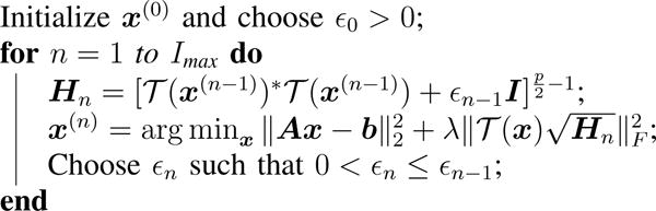
for all 0 < p ≤ 1, provided X has no zero singular values so that H is well-defined. Here $\sqrt{\mathit{H}}$ denotes any matrix³ satisfying $\mathit{H}=\left(\sqrt{\mathit{H}}\right)\left(\sqrt{\mathit{H}}\right)\ast$. This suggests an iterative algorithm for minimizing the Schatten-p quasi-norm that alternates between updating a weight matrix H and solving a weighted least squares problem with H fixed. In particular, substituting $\mathit{X}=\mathcal{T}\left(\mathit{x}\right)$ in the IRLS-p algorithm presented in [21] gives the following iterative scheme for solving (16):

$${\mathit{H}}_n={[\mathcal{T}{\left({\mathit{x}}^{\left(n-1\right)}\right)}^{\ast }\mathcal{T}\left({\mathit{x}}^{(n-1)}\right)]}^{\frac{p}{2}-1}$$

$${\mathit{x}}^{(n)}=\underset{\mathit{x}}{\arg min}{\Vert \mathit{A}\mathit{x}-\mathit{b}\Vert }_2^2+\lambda {\Vert \mathcal{T}\left(\mathit{x}\right)\sqrt{{\mathit{H}}_n}\Vert }_F^2.$$

To ensure the matrix defining H_n is invertible, and to improve numerical stability, following the approach in [21] we introduce a smoothing parameter ε_n > 0 to the H-update as ${\mathit{H}}_n={\left(\mathcal{T}\left({\mathit{x}}^{\left(n-1\right)}\right)\ast \mathcal{T}\left({\mathit{x}}^{\left(n-1\right)}\right)+{\epsilon }_n\mathit{I}\right)}^{-\frac{1}{2}}$, satisfying ε_n → 0 as n → ∞. Pseudo-code summarizing this approach is given in Algorithm 1. In the Appendix we show that the IRLS-p algorithm can be derived as a majorization-minimization (MM) algorithm [49] for the objective (16). Due to properties of MM algorithms, this ensures that the IRLS-p iterates monotonically decrease the cost function (12). Moreover, in the convex case p = 1 (i.e. nuclear norm regularization), the iterates are guaranteed to converge to the global minimum of (16); in the non-convex case p ∈ [0, 1), convergence to the global optimality cannot be ensured, but the iterates are still guaranteed to converge to a stationary point. We refer the reader to [21], [22] for a more detailed convergence analysis of the IRLS-p algorithm in the context of low-rank matrix completion.

Algorithm 1.

IRLS-p algorithm for structured low-rank matrix recovery

A. Challenges with the direct IRLS approach

While the IRLS-p algorithm has shown several advantages in the low-rank matrix completion setting [20]–[22], the direct adaptation of IRLS-p to the structured matrix liftings considered in this work is computationally prohibitive for large-scale problems. To see why, first note that the weight matrix update requires computing an inverse power of the Gram matrix $\mathcal{T}\left(\mathit{x}\right)\ast \mathcal{T}\left(\mathit{x}\right)\in {ℂ}^{N\times N}$. Computing this Gram matrix directly by matrix multiplication will be costly when the inner dimension M ≫ N, and inverting the resulting matrix can be unstable due to round-off errors. Instead, a more stable and efficient method to compute the inverse is by an SVD of the M ×N matrix $\mathcal{T}\left(\mathit{x}\right)$, which requires O(MN²) flops to compute. In the case that $\mathcal{T}\left(\mathit{x}\right)$ is approximately low-rank, one can instead compute only the top r singular values and singular vectors either using deterministic methods, such as Lanczos bidiagonalization [50], or by randomized methods [51], at a reduced cost of O(MNr) flops. However, these approaches are still dominated by a computational cost that is linear in M, and will still be prohibitively slow when M is large or when the matrix $\mathcal{T}\left(\mathit{x}\right)$ is not sufficiently low-rank. Note these are the same fundamental costs involved in other SVD-based algorithms for structured low-rank matrix recovery; see the Supplementary Materials for more details.

The IRLS-p algorithm additionally requires solving the following least-squares problem at each iteration:

$$\underset{\mathit{x}}{min}{\Vert \mathit{A}\mathit{x}-\mathit{b}\Vert }^2+\lambda {\Vert \mathcal{T}\left(\mathit{x}\right)\sqrt{\mathit{H}}\Vert }_F^2.$$ (22)

To give an idea of the costs involved in solving (22) via an iterative solver, consider the case where the matrix lifting has the form $\mathcal{T}\left(\mathit{x}\right)={\text{Toep}}_d\left(\mathit{x}\right)$, i.e., $\mathcal{T}\left(\mathit{x}\right)\mathit{h}=\mathit{x}\ast \mathit{h}$. The challenge is that standard iterative methods for solving (22), such as the CG or LSQR algorithm [52], would require O(N) multi-dimensional FFTs per iteration, where N = |Λ| is the total number of filter coefficients. However, N can be on the order of hundreds or thousands for the problems considered in this work. Therefore, standard methods for solving the least-squares problem (22) will also be prohibitively costly for large-scale problems.

IV. Proposed GIRAF Algorithm

As observed in the previous section, the direct IRLS algorithm will not scale well to large problem instances because of two challenges: 1) computing the weight matrix update requires a large-scale SVD, and 2) computing a solution to the least squares problem requires a prohibitive number of FFTs. In this section we propose a novel approximation of the problem formulation (16) to overcome these difficulties. The main idea is to approximate the structured matrix lifting $\mathcal{T}$ in a systematic way such that the complexity of the resulting IRLS subproblems simplify, while preserving the rank structure of the lifting as best as possible.

A. Half-circulant approximation of a Toeplitz matrix

Our approximation is based on the observation that every multi-level Toeplitz matrix can be embedded in a larger multi-level circulant matrix. Specifically, the d-level Toeplitz matrix Toep_d(y) built with filter support Λ ⊂ ℤ^d and valid index set Γ ⊂ ℤ^d can always be expressed as:

$${\text{Toep}}_d\left(\mathit{y}\right)={\mathit{P}}_{\mathrm{\Gamma }}\mathit{C}\left(\mathit{y}\right){\mathit{P}}_{\mathrm{\Lambda }}^{\ast }$$ (23)

Here C(y) ∈ ℂ^L×L is a matrix representing convolution with the array y, P_Γ ∈ ℂ^M×L is a matrix representing restriction to valid set Γ, and ${\mathit{P}}_{\mathrm{\Lambda }}^{\ast }\in {ℂ}^{L\times N}$ represents a zero-padding outside the filter support Λ. The matrices P_Γ and ${\mathit{P}}_{\mathrm{\Lambda }}^{\ast }$ act as row-restriction and column-restriction operators, respectively; see Figure (3) for an illustration. Because of the restriction matrix P_Γ, we can assume C(y) represents a multi-dimensional circular convolution, i.e., C(y) is multi-level circulant, provided the convolution takes place on a sufficiently large rectangular grid to avoid wrap-around boundary effects. In particular, the rectangular circular convolution grid should be at least as large as the data support Δ ⊂ ℤ^d. Without loss of generality, from now on we assume the data support Δ is rectangular so that it coincides with the circular convolution grid.

Fig. 3. Example of Half-circulant approximation in 1-D.

We approximate the Toeplitz matrix lifting $\mathcal{T}\left(\mathit{x}\right)$ with the half-circulant matrix $\stackrel{⌣}{\mathcal{T}}\left(\mathit{x}\right)$ obtained by adding rows to $\mathcal{T}\left(\mathit{x}\right)$ to make it the full vertical section of a circulant matrix C(Mx)

To simplify subsequent derivations, in this section we assume the structured matrix lifting $\mathcal{T}\left(\mathit{x}\right)$ consists of a single multi-level Toeplitz block: $\mathcal{T}\left(\mathit{x}\right)={\text{Toep}}_d\left(\mathit{M}\mathit{x}\right)$. According to (23), $\mathcal{T}\left(\mathit{x}\right)$ can be written as

$$\mathcal{T}\left(\mathit{x}\right)={\mathit{P}}_{\mathrm{\Gamma }}\mathit{C}\left(\mathit{M}\mathit{x}\right){\mathit{P}}_{\mathrm{\Lambda }}^{\ast }$$ (24)

We propose approximating the structured matrix lifting $\mathcal{T}\left(\mathit{x}\right)$ with the surrogate lifting $\stackrel{⌣}{\mathcal{T}}\left(\mathit{x}\right)$ defined by

$$\stackrel{⌣}{\mathcal{T}}\left(\mathit{x}\right)=\mathit{C}\left(\mathit{M}\mathit{x}\right){\mathit{P}}_{\mathrm{\Lambda }}^{\ast }$$ (25)

i.e., we omit the left-most row restriction operator P_Γ from $\mathcal{T}\left(\mathit{x}\right)$ so that $\stackrel{⌣}{\mathcal{T}}\left(\mathit{x}\right)$ is the full vertical section of the multi-level circulant matrix C(Mx). In general, we say a matrix X ∈ ℂ^{M ×N}, N ≤ M, is (multi-level) half-circulant if it can be written as X = CP*, where C ∈ ℂ^M×M is (multi-level) circulant and P ∈ ℂ^N×M is a restriction matrix, i.e., X is obtained by selecting N full columns from C.

Inserting the approximation (25) into (16), we propose solving

$$\underset{x}{min}{\Vert \mathit{A}\mathit{x}-\mathit{b}\Vert }^2+\lambda {\Vert \stackrel{⌣}{\mathcal{T}}\left(\mathit{x}\right)\Vert }_p^p.$$ (26)

using the IRLS-p algorithm. In other words, rather than penalizing the Schatten-p norm of the exact multilevel Toeplitz lifted matrix, we penaltize its multi-level half-circulant approximation instead. We can justify this approach by considering the effect the half-circulant approximation (25) has on the singular values of the lifting. Recall that C(y) denotes circular convolution with the array y on a rectangular grid Δ ⊂ ℤ^d containing the index set Γ. Hence, after a rearrangement of rows, we can always write $\mathcal{T}\left(\mathit{x}\right)$ submatrix of $\stackrel{⌣}{\mathcal{T}}\left(\mathit{x}\right)$:

$$\stackrel{⌣}{\mathcal{T}}\left(\mathit{x}\right)=\left[\begin{array}{c}\mathcal{T}\left(\mathit{x}\right)\\ ℬ\left(\mathit{x}\right)\end{array}\right]=\left[\begin{array}{c}{\mathit{P}}_{\mathrm{\Gamma }}\mathit{C}\left(\mathit{M}\mathit{x}\right){\mathit{P}}_{\mathrm{\Lambda }}^{\ast }\\ {\mathit{P}}_{{\mathrm{\Gamma }}^C}\mathit{C}\left(\mathit{M}\mathit{x}\right){\mathit{P}}_{\mathrm{\Lambda }}^{\ast }\end{array}\right],$$ (27)

where Γ^C is the set complement of Γ inside the circular convolution grid Δ. In other words, $\stackrel{⌣}{\mathcal{T}}\left(\mathit{x}\right)$ is the unique matrix obtained by augmenting the rows of $\mathcal{T}\left(\mathit{x}\right)$ to make it (multi-level) half-circulant.

As a consequence of the embedding (27), the singular values of $\mathcal{T}\left(\mathit{x}\right)$ are bounded by those of $\stackrel{⌣}{\mathcal{T}}\left(\mathit{x}\right)$:

$${\sigma }_i\left(\mathcal{T}\left(\mathit{x}\right)\right)\le {\sigma }_i\left(\stackrel{⌣}{\mathcal{T}}\left(\mathit{x}\right)\right)\text{for}i=1,\dots ,N.$$ (28)

(see Corollary 3.1.3 in [53]). Hence, the Schatten-p quasi-norm of $\mathcal{T}\left(\mathit{x}\right)$ is also bounded by that of $\stackrel{⌣}{\mathcal{T}}\left(\mathit{x}\right)$:

$${\Vert \mathcal{T}\left(\mathit{x}\right)\Vert }_p^p\le {\Vert \stackrel{⌣}{\mathcal{T}}\left(\mathit{x}\right)\Vert }_p^p\text{for}\text{all}0\le p\le 1.$$ (29)

Moreover, if in minimizing ${\Vert \stackrel{⌣}{\mathcal{T}}\left(\mathit{x}\right)\Vert }_p^p$ we obtain a low-rank matrix $\stackrel{⌣}{\mathcal{T}}\left({\mathit{x}}^{\prime }\right)$ with rank r, the singular value bounds (28) show that $\mathcal{T}\left({\mathit{x}}^{\prime }\right)$ is also low-rank with rank ≤ r. This shows that it is reasonable to use ${\Vert \stackrel{⌣}{\mathcal{T}}\left(\mathit{x}\right)\Vert }_p^p$ as a surrogate penalty for ${\Vert \mathcal{T}\left(\mathit{x}\right)\Vert }_p^p$.

Empirically, we find that when the data support is sufficiently large relative to the filter size, i.e., when M ≫ N where $\mathcal{T}\left(\mathit{x}\right)\in {ℂ}^{M\times N}$, then using the surrogate lifting $\stackrel{⌣}{\mathcal{T}}\left(\mathit{x}\right)$ results in negligible approximation errors (see Figure 6). When the data support Δ is small, we recommend solving for the data array x on a slightly larger “oversampled” grid Δ′ to keep the approximation error low. Typically we take Δ′ = Δ+2Λ, i.e. we pad the data support with an extra margin having the size of the filter support. After solving the problem on the oversampled grid Δ′, we finally restrict the solution to the desired data support Δ. We study the effect of using an oversampled grid in Section V (see Figure 7).

Fig. 6.

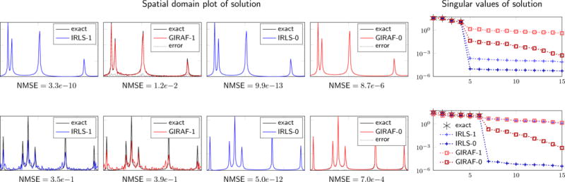
Comparison of solutions obtained by the IRLS-p and the GIRAF-p algorithm, p = 1, 0, for recovery of Fourier coefficients of r Diracs, as in (1), from non-uniform random Fourier samples. The top row shows an experiment (r = 4, 50% random samples) where both IRLS-1 and IRLS-0 succeed in recovering the signal. In this case the GIRAF-1 algorithm shows non-negligible approximation errors, but the GIRAF-0 result is close to exact. The bottom row shows an experiment (r = 6, 33% random samples) where IRLS-1 fails, but IRLS-0 is successful; similarly, the GIRAF-1 recovery fails, while the GIRAF-0 result is again close to exact. Shown in the right column are the singular values of the exact matrix lifting $\mathcal{T}\left({\mathit{x}}^{\star }\right)$ where x^⋆ is the solution obtained from each algorithm. Note GIRAF-0 solutions are still approximately low-rank under the exact lifting.

Fig. 7.

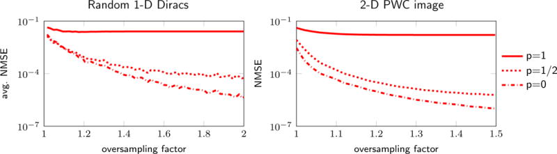
Reconstruction error versus oversampling factor for GIRAF-p algorithm on the recovery of synthetic low-rank data. The quality of the half-circulant approximation (25) used in the GIRAF-p algorithms improves by working on an oversampled grid, i.e., increasing the number of rows in the half-circulant matrix lifting. The left plot corresponds to the recovery Fourier coefficients of Diracs in 1-D, using the same settings as in Figure 6; we report the average NMSE over 50 random trials. The right plot shows recovery of Fourier coefficients of a synthetic 2-D piecewise constant image using the gradient weighted lifting (9). Observe that the NMSE stagnates for the p = 1 case (convex penalty). However, the NMSE diminishes towards zero with the oversampling factor when p = 0.5 and p = 0 (non-convex penalties). This suggests it is important to use the non-convex versions of GIRAF on a sufficiently large oversampled grid to mitigate errors due to the half-circulant approximation.

We now show the IRLS algorithm applied to (26) results in subproblems with significantly reduced complexity due to the half-circulant structure of the approximated lifting. In particular, we will show the algorithm can be interpreted as alternating between: (1) solving for an annihilating filter for the data, and (2) solving for the data best annihilated by the filter in a least-squares sense. Due to this interpretation, we call this approach the Generic Iterative Reweighted Annihilating Filter (GIRAF) algorithm.

B. GIRAF least squares subproblem

1) Reformulation as least squares annihilation

For a fixed weight matrix H, the GIRAF least squares subproblem has the form

$$\underset{\mathit{x}}{min}{\Vert \mathit{A}\mathit{x}-\mathit{b}\Vert }_2^2+\lambda {\Vert \stackrel{⌣}{\mathcal{T}}\left(\mathit{x}\right)\sqrt{\mathit{H}}\Vert }_F^2$$ (30)

Under the half-circulant assumption (25), we can re-express the Frobenius norm above as

$${\Vert \stackrel{⌣}{\mathcal{T}}\left(\mathit{x}\right){\mathit{H}}^{\frac{1}{2}}\Vert }_F^2={\displaystyle \sum _{i=1}^N{\Vert \stackrel{⌣}{\mathcal{T}}\left(\mathit{x}\right){\mathit{h}}_i\Vert }_2^2}={\displaystyle \sum _{i=1}^N{\Vert \mathit{C}\left(\mathit{M}\mathit{x}\right){\mathit{P}}_{\mathrm{\Lambda }}^{\ast }{\mathit{h}}_i\Vert }_2^2}$$ (31)

where h_i is the ith column of $\sqrt{\mathit{H}}$. Because circular convolution is commutative, we can write $\mathit{C}\left(\mathit{M}\mathit{x}\right){\mathit{P}}_{\mathrm{\Lambda }}^{\ast }{\mathit{h}}_i={\mathit{C}}_i\mathit{M}\mathit{x}$, where ${\mathit{C}}_i:=\mathit{C}\left({\mathit{P}}_{\mathrm{\Lambda }}^{\ast }{\mathit{h}}_i\right)$ is a multi-level circulant matrix representing circular convolution with the zero-padded filter h_i on the rectangular grid Δ ⊂ ℤ^d. Therefore, C_i = F D_iF^∗ where F is the DFT on Δ, and D_i the diagonal matrix having entries given by the array ${\mathit{d}}_i=\mathit{F}\ast {\mathit{P}}_{\mathrm{\Lambda }}^{\ast }{\mathit{h}}_i$, the inverse DFT of the zero-padded filter h_i. This allows us to simplify the right-hand side of (31) as

$${\displaystyle \sum _{i=1}^N{\Vert {\mathit{C}}_i\mathit{M}\mathit{x}\Vert }_2^2={\mathit{x}}^{\ast }{\mathit{M}}^{\ast }}\left({\displaystyle \sum _{i=1}^N{\mathit{C}}_i^{\ast }{\mathit{C}}_i}\right)\mathit{M}\mathit{x}={\mathit{x}}^{\ast }{\mathit{M}}^{\ast }\mathit{F}\left({\displaystyle \sum _{i=1}^N{\mathit{D}}_i^{\ast }{\mathit{D}}_i}\right){\mathit{F}}^{\ast }\mathit{M}\mathit{x}={\Vert {\mathit{D}}^{\frac{1}{2}}{\mathit{F}}^{\ast }\mathit{M}\mathit{x}\Vert }_2^2,$$

where we have set $\mathit{D}={\displaystyle {\sum }_{i=1}^N{\mathit{D}}_i^{\ast }{\mathit{D}}_i}$, which is again diagonal with entries d ∈ ℂ^|Δ| given by

$$\mathit{d}={\displaystyle \sum _{i=1}^N{\left|{\mathit{d}}_i\right|}^2,{\mathit{d}}_i={\mathit{F}}^{\ast }{\mathit{P}}_{\mathrm{\Lambda }}^{\ast }{\mathit{h}}_i}\text{for}\text{all}i=1,\dots ,N,$$ (32)

where |·| is applied element-wise. Therefore, (30) transforms into the weighted least squares problem:

$$\underset{\mathit{x}}{min}{\Vert \mathit{A}\mathit{x}-\mathit{b}\Vert }_2^2+\lambda {\Vert {\mathit{D}}^{\frac{1}{2}}{\mathit{F}}^{\ast }\mathit{M}\mathit{x}\Vert }_2^2.$$ (33)

Observe that by making use of the half-circulant assumption we have effectively reduced the working dimension of the least-squares problem back down to the dimension of the original decision variable x.

Computing the weights d according to the formula (32) can be costly for large-scale problems since it requires N large-scale FFTs. A more efficient approach is to pre-compute the filter h defined by

$$\mathit{h}={\displaystyle \sum _{i=1}^N\left({\stackrel{\sim }{\mathit{h}}}_i\ast {\mathit{h}}_i\right)}$$ (34)

where ${\stackrel{\sim }{\mathit{h}}}_i$ is the reversed, conjugated filter defined by ${\stackrel{\sim }{\mathit{h}}}_i[\mathit{k}]=\overline{{\mathit{h}}_i[-\mathit{k}]}$ for all k ∈ Λ. Note that h has coefficients supported within 2Λ:= {k + ℓ: k, ℓ ∈ Λ} since each h_i is supported within Λ. Therefore, applying the DFT convolution theorem to (32), d can be obtained by $\mathit{d}={\mathit{F}}^{\ast }{\mathit{P}}_{2\mathrm{\Lambda }}^{\ast }\mathit{h}$, which after computing h, requires only one large-scale FFT. We call filter h defined in (34) the re-weighted annihilating filter and d the annihilation weights.

2) ADMM solution of least-squares annihilation

The linear least-squares problem (33) can be readily solved with an off-the-shelf solver, such as the CG or LSQR algorithm [52]. However, the problem is poorly conditioned when the annihilation weights d are close to zero, which is expected to happen as the iterations progress. Therefore, solving (33) efficiently during the course of the GIRAF algorithm will require a robust preconditioning strategy. However, because the transformation M is not always invertible, designing an all-purpose preconditioner for (33) is challenging. Instead, we adopt an approach which allows us to solve a series of subproblems with predictably good conditioning. The approach is based on the following variable splitting:

$$\underset{\mathit{x}}{min}{\Vert \mathit{A}\mathit{x}-\mathit{b}\Vert }_2^2+\lambda {\Vert {\mathit{D}}^{\frac{1}{2}}\mathit{y}\Vert }_2^2\text{subject to}\mathit{F}\mathit{y}=\mathit{M}\mathit{x}.$$ (35)

The equality constrained problem (35) can be efficiently solved with the alternating directions method of mulipliers (ADMM) algorithm [54], which results in the following iterative scheme:

$${\mathit{y}}^{\left(n\right)}=\underset{\mathit{y}}{\arg min}\left\{{\Vert {\mathit{D}}^{\frac{1}{2}}\mathit{y}\Vert }_2^2+\gamma {\Vert \mathit{y}-{\mathit{F}}^{\ast }\mathit{M}{\mathit{x}}^{(n-1)}+{\mathit{q}}^{\left(n-1\right)}\Vert }_2^2\right\},$$ (36)

$${\mathit{x}}^{\left(n\right)}=\underset{\mathit{x}}{\arg min}\left\{{\Vert \mathit{A}\mathit{x}-\mathit{b}\Vert }_2^2+\gamma \lambda {\Vert {\mathit{y}}^{(n)}-{\mathit{F}}^{\ast }\mathit{M}\mathit{x}+{\mathit{q}}^{(n-1)}\Vert }_2^2\right\},$$ (37)

$${\mathit{q}}^{(n)}={\mathit{q}}^{(n-1)}+\mathit{F}{\mathit{y}}^{(n)}-\mathit{M}{\mathit{x}}^{(n)},$$ (38)

where q represents a vector of Lagrange multipliers, and γ > 0 is a fixed parameter that can be tuned to improve the conditioning of the subproblems. Subproblems (36) and (37) are both quadratic and can be solved efficiently: (36) has the exact solution

$${\mathit{y}}^{(n)}={\left(\mathit{D}+\gamma \mathit{I}\right)}^{-1}\left(\gamma {\mathit{F}}^{\ast }\left[\mathit{M}{\mathit{x}}^{(n-1)}-\mathit{q}\right]\right).$$ (39)

Since D + γI is diagonal, its inverse acts as an element-wise division. Likewise, the solution of (37) can be obtained as

$${\mathit{x}}^{(n)}={\left({\mathit{A}}^{\ast }\mathit{A}+\lambda \gamma {\mathit{M}}^{\ast }\mathit{M}\right)}^{-1}\left[{\mathit{A}}^{\ast }\mathit{b}+\lambda \gamma {\mathit{M}}^{\ast }\mathit{F}\left({\mathit{y}}^{(n)}+{\mathit{q}}^{(n-1)}\right)\right].$$ (40)

In many problems of interest, both A^∗A and M^∗M are diagonal, which means x⁽ⁿ⁾ is also obtained by an efficient element-wise division. In this case, aside from the element-wise operations, the computational cost of one pass of ADMM iterations (36)–(38) is three FFTs. When either A^∗A or M^∗M are not diagonal, an approximate solution to (37) can be found by a few passes of an iterative solver instead. Even with inexact updates of the x-subproblem, we are still guaranteed convergence of the overall ADMM algorithm under fairly broad conditions; see, e.g., [54], [55].

Update (39) suggests choosing γ adaptively before solving each ADMM subproblem according to the magnitude of the annihilation weights $\mathit{d}={\left\{d_j\right\}}_{j=1}^L$ of D to ensure good conditioning and fast convergence of the ADMM scheme. We recommend choosing γ = (max_j d_j)/δ for δ ≥ 1; we study the effect of δ in Section V.

C. GIRAF re-weighted annihilating filter subproblem

1) Construction of Gram matrix

At each iteration, the GIRAF algorithm requires updating a weight matrix H according to:

$$\mathit{H}={\left(\stackrel{⌣}{\mathcal{T}}{\left(\mathit{x}\right)}^{\ast }\stackrel{⌣}{\mathcal{T}}\left(\mathit{x}\right)+\epsilon \mathit{I}\right)}^{\frac{p}{2}-1}$$ (41)

Rather than computing H via a full or partial SVD of the tall M × N matrix $\stackrel{⌣}{\mathcal{T}}\left(\mathit{x}\right)$, as is recommended in [21], we propose computing H via the eigendecomposition of the smaller N × N Gram matrix $\mathit{G}=\stackrel{⌣}{\mathcal{T}}{\left(\mathit{x}\right)}^{\ast }\stackrel{⌣}{\mathcal{T}}\left(\mathit{x}\right)$. This is because the half-circulant approximation (25) allows us to compute G efficiently in a matrix-free manner, as we now show. From (25), we have

$$\mathit{G}={\mathit{P}}_{\mathrm{\Lambda }}\mathit{C}{\left(\mathit{M}\mathit{x}\right)}^{\ast }\mathit{C}\left(\mathit{M}\mathit{x}\right){\mathit{P}}_{\mathrm{\Lambda }}^{\ast }.$$ (42)

The restriction matrices P_Λ and ${\mathit{P}}_{\mathrm{\Lambda }}^{\ast }$ in (42) extract an N × N block of C(Mx)^∗C(Mx) corresponding to the intersection of the rows and columns indexed by the filter support set Λ. Note that the product C(Mx)^∗C(Mx) = C(g) is again a multi-level circulant matrix whose entries are generated by the array g = F |F ^∗ Mx|² with the operation |·|² is understood element-wise. Therefore, we can build G by performing a sliding-window operation that extracts every patch of size Λ from the array g. In particular, because of the restriction matrices P_Λ and ${\mathit{P}}_{\mathrm{\Lambda }}^{\ast }$ in (42), we only need to consider patches coming from g restricted to the index set 2Λ = {k + ℓ: k, ℓ ∈ Λ}. Aside from this sliding-window operation, the main cost in computing G is two FFTs.

2) Update of re-weighted annihilating filter

According to section IV-B, the GIRAF least squares subproblem can be interpreted as an annihilation of the data subject to a filter h determined by the columns h₁, …, h_N of $\sqrt{\mathit{H}}$. We now show how to update h directly from an eigendecomposition of the Gram matrix $\mathit{G}=\stackrel{⌣}{\mathcal{T}}{\left(\mathit{x}\right)}^{\ast }\stackrel{⌣}{\mathcal{T}}\left(\mathit{x}\right)$, rather than forming $\sqrt{\mathit{H}}$ explicitly. Let G = V Λ V^∗ where the columns ${\left\{{\mathit{v}}_i\right\}}_{i=1}^N$ of V are an orthonormal basis of eigenvectors and Λ is diagonal matrix of the associated eigenvalues ${\left\{{\lambda }_i\right\}}_{i=1}^N$. Then the weight matrix update (41) reduces to

$$\mathit{H}={\left[\mathit{V}\left(\mathbf{\Lambda }+\epsilon \mathit{I}\right){\mathit{V}}^{\ast }\right]}^{\frac{p}{2}-1}=\mathit{V}{\left(\mathbf{\Lambda }+\epsilon \mathit{I}\right)}^{\frac{p}{2}-1}{\mathit{V}}^{\ast }.$$ (43)

One choice of the matrix square root $\sqrt{\mathit{H}}$ is

$$\sqrt{\mathit{H}}=\mathit{V}{\left(\mathbf{\Lambda }+\epsilon \mathit{I}\right)}^{-\frac{q}{2}}=[{\left({\lambda }_1+\epsilon \right)}^{-\frac{q}{2}}{\mathit{v}}_1,\dots ,{\left({\lambda }_M+\epsilon \right)}^{-\frac{q}{2}}{\mathit{v}}_M].$$ (44)

where $q=1-\frac{p}{2}$. However, the least squares subproblem of the algorithm only needs as input the filter h defined in (34), which is determined by the columns h_i of $\sqrt{\mathit{H}}$. Making the substitutions ${\mathit{h}}_i={\left({\lambda }_1+\epsilon \right)}^{-\frac{q}{2}}{\mathit{v}}_i$ in (34) gives the following update:

$$\mathit{h}={\displaystyle \sum _{i=1}^N{\left({\lambda }_i+\epsilon \right)}^{-q}\left({\stackrel{\sim }{\mathit{v}}}_i\ast {\mathit{v}}_i\right);q=1-\frac{p}{2}.}$$ (45)

Note that the weight (λ_i + ε)^−q, q > 0, is large only when the filter v_i is close to the null space of $\stackrel{⌣}{\mathcal{T}}\left(\mathit{x}\right)$, i.e., when v_i is an annihilating filter. Therefore, h can be thought of as a weighted average of all the annihilating filters for $\stackrel{⌣}{\mathcal{T}}\left(\mathit{x}\right)$. Notice that the only effect of changing the Schatten-p penalty parameter 0 ≤ p ≤ 1 is to change the exponent q in the computation of (45). Smaller values of p (larger values of q) are more likely to promote low-rank solutions at the iterations progress, since the weights on the filters close to the null space will be higher; see Figure 4 for an illustration of this effect.

Fig. 4.

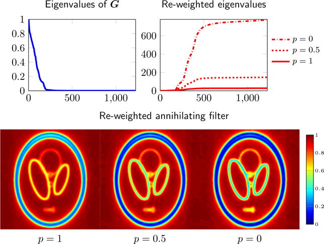
Effect of Schatten-p penalty on the GIRAF re-weighted annihilating filter. We show the eigenvalues of $\mathit{G}=\stackrel{⌣}{\mathcal{T}}{\left(\mathit{x}\right)}^{\ast }\stackrel{⌣}{\mathcal{T}}\left(\mathit{x}\right)$ during one iteration of the GIRAF algorithm applied to the gradient weighted lifting (9) (top left), and the different re-weightings of the eigenvalues specified by different Schatten-p penalties (top right). The set of annihilation weights determined by the resulting re-weighted annihilating filter given by (45) are shown in the bottom row, normalized to [0, 1]. Note that for smaller values of p the annihilation weights are closer to zero near the edges because the re-weighted annihilating filter gives higher weight to filters in the nullspace of $\stackrel{⌣}{\mathcal{T}}\left(\mathit{x}\right)$

Algorithm 2.

GIRAF-p algorithm for structured low-rank matrix recovery

D. Extension to liftings with multiple blocks

To simplify the derivation of the GIRAF algorithm we assumed that the original matrix lifting $\mathcal{T}\left(\mathit{x}\right)$ consists of a single multi-level Toeplitz block. However, the GIRAF algorithm can easily be modified to accommodate liftings with a vertical block structure, as in (19), by applying the half-circulant approximation to each block. In this case, one can show the GIRAF least-squares problem simplifies to

$$\underset{\mathit{x}}{min}{\Vert \mathit{A}\mathit{x}-\mathit{b}\Vert }_2^2+\lambda {{\displaystyle \sum _{i=1}^K}\Vert {\mathit{D}}^{\frac{1}{2}}{\mathit{F}}^{\ast }{\mathit{M}}_i\mathit{x}\Vert }_2^2.$$ (46)

where D = diag(d), and the annihilation weights d are computed the same as in (32) and (45) from an eigendecomposition of the Gram matrix $\mathit{G}={\displaystyle {\sum }_{i=1}^K{\stackrel{⌣}{\mathcal{T}}}_i{\left(\mathit{x}\right)}^{\ast }{\stackrel{⌣}{\mathcal{T}}}_i\left(\mathit{x}\right)}$.

E. Implementation Details

An overview of the GIRAF algorithm is given in Algorithm 2. Empirically we find that several of the heuristics in [44] for setting the smoothing parameter ε_n work well for the GIRAF algorithm, as well. In particular, we set ε₀ = λ_max/100 where λ_max is the maximum eigenvalue of the Gram matrix $\stackrel{⌣}{\mathcal{T}}{\left({\mathit{x}}^{\left(0\right)}\right)}^{\ast }\stackrel{⌣}{\mathcal{T}}\left({\mathit{x}}^{\left(0\right)}\right)$, which is obtained as a by-product of the first iterate of the algorithm. We recommend decreasing the smoothing parameter ε_n exponentially as ε_n = ε₀ (η)⁻ⁿ, where η > 1 is a fixed parameter. We find that η = 1.3 is suitable for a wide range of problem instances. The ADMM approach for solving the GIRAF least-squares subproblem also requires a conditioning parameter δ. We typically set δ = 100, which was found to represent a desirable trade-off between speed and accuracy for a wide range of problem instances; see Figure 5.

Fig. 5.

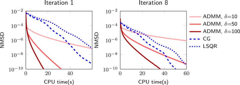
Computation time comparison for solvers of the GIRAF least-squares problem. We study the least-squares problem arising in iterations 1 and 8 of the GIRAF algorithm applied to a Fourier recovery experiment. The proposed ADMM approach shows nearly ten-fold increase in the rate at which NMSD is decreased over CG and LSQR, provided the pre-conditioning parameter δ is chosen correctly.

V. Numerical experiments

In this section we perform several experiments to investigate properties of the GIRAF algorithm, and compare with other algorithms for structured low-rank matrix recovery. All experiments were conducted in MATLAB 8.5.0 (R2015a) on a Linux desktop computer with a Intel Xeon 3.20GHz CPU and 24 GB RAM.

A. Behavior of GIRAF algorithm

1) Half-circulant approximation, oversampled grid, and choice of p

The GIRAF algorithm relies on a half-circulant approximation (25) of Toeplitz matrix liftings. Here we investigate the error induced by this approximation in a 1-D signal recovery setting, where the matrix lifting is single-level Toeplitz: $\mathcal{T}\left(\mathit{x}\right)=\text{Toep}\left(\mathit{x}\right)$. We randomly undersample the exact Fourier coefficients ${\mathit{x}}_0=\left(\widehat{\rho }\left[k\right]:\left|k\right|<64\right)$ of a 1-D stream of r Diracs ρ(x) as in (1), and attempt to recover the missing samples by applying the IRLS-p to the Toeplitz matrix lifting $\mathcal{T}\left(\mathit{x}\right)$ having dimensions 113 × 15, and by using the GIRAF-p algorithm, which is equivalent to applying IRLS-p to the half-circulant approximated lifting $\stackrel{⌣}{\mathcal{T}}\left(\mathit{x}\right)$ having dimensions 157 × 15. We observe the IRLS-0 algorithm generally outperforms the IRLS-1, consistent with the results in [21]. Furthermore, the quality of the GIRAF-p reconstructions mimics those obtained with IRLS-p, but with small approximation errors. However, the approximation error is noticeably less severe in the non-convex p = 0 case.

We investigate this phenomenon in another experiment shown in Figure 7. Using the same experimental setup, we varied the working grid size of the problem, i.e., we varied the size of the oversampled reconstruction grid Δ′ defined in Section IV-A; this only changes the number of rows M in the lifting $\stackrel{⌣}{\mathcal{T}}\left(\mathit{x}\right)$. We vary M = 127, …, 255, corresponding to a maximum oversampling factor of 2. For the convex GIRAF-1 algorithm, we find that the reconstruction error stagnates with respect to the oversampling factor. However, for the non-convex GIRAF-p algorithms, p < 1, the reconstruction diminishes significantly with the oversampling factor. We additionally perform a similar experiment using the gradient weighted lifting scheme (9) on synthetic data that is piecewise constant and known to be low-rank in the lifted domain (the SL dataset shown in Figure 9) with data size 201 × 201, filter size 25 × 25, and 50% random samples. In this case we also obtain similar results—the nonconvex GIRAF algorithms achieve substantially smaller approximation errors that decrease with the oversampling factor. While this suggests one should use a very large oversampled grid to eliminate approximation errors, there is a trade-off with computational cost, since the oversampled grid represents the working dimension of the problem. The extent of oversampling will depend on the problem setting and required precision.

Fig. 9.

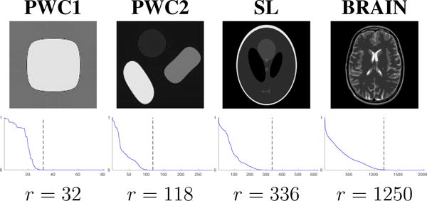
Synthetic piecewise constant images used in structured low-rank recovery experiments. Shown below the images are the normalized singular value spectrum of the gradient weighted lifted matrix constructed from the fully sampled Fourier coefficients, where the dotted line indicates the rank estimate r.

These experiments suggest it is better to use a non-convex GIRAF-p, 0 ≤ p < 1, algorithm over the convex GIRAF-1 algorithm in order to mitigate errors due to the half-circulant approximation. In the remainder of our experiments we focus on the GIRAF-0 algorithm, since it yielded the lowest reconstruction error in most cases.

2) ADMM approach to GIRAF least-squares solution

In Figure 5 we compare the computation time of the proposed ADMM approach (36)–(38) for solving the GIRAF least-square subproblem (33) against standard CG and LSQR solvers. Here we investigate the GIRAF-0 algorithm applied to a Fourier domain recovery experiment using the gradient weighted lifting scheme (9). We take the measurement operator A to be a Fourier domain sampling, and sample 25% of the data uniformly at random, using the Shepp-Logan phantom (data size 256×256 and filter size of 35×35). The metric used to evaluate each approach is the normalized mean-square difference $\text{NMSD}={\Vert \mathit{x}-{\mathit{x}}_{\ast }\Vert }^2/{\Vert {\mathit{x}}_{\ast }\Vert }^2$ where x is the current iterate, and x_* is the true solution, which was obtained by running CG algorithm to high precision. The proposed ADMM approach shows nearly a ten-fold increase in over CG and LSQR. The rate at which the ADMM approach reduces the NMSD shows some sensitivity to the parameter δ, but only in the high-accuracy regime (NMSD < 10⁻⁴).

B. Recovery Experiments

To demonstrate the benefits of the GIRAF algorithm for structured low-rank matrix recovery, we focus on the problem of undersampled MRI reconstruction in 2-D. In this setting, the goal is to recover an array x₀ of the Fourier coefficients of an image from missing or corrupted Fourier samples. In addition to the direct IRLS-p algorithm (see Algorithm 1), we compare GIRAF against the following algorithms proposed for structured low-rank matrix recovery:

• Alternating projections (AP). Also known as Cadzow’s method [56], this approach was adopted for noisy finite-rate-of-innovation (FRI) signal recovery in [37], [57], [58], and for auto-calibrated parallel MRI reconstruction in [2]. Reconstruction in an AP algorithm is posed as

  $$\underset{\mathit{x}}{min}{\Vert \mathit{A}\mathit{x}-\mathit{b}\Vert }^2\text{subject to}\{\begin{array}{l}\mathit{X}=\mathcal{T}\left(\mathit{x}\right)\\ \text{rank}\mathit{X}\le r,\end{array}$$ (47)

  which is solved by alternately projecting X onto: (1) the set of matrices with rank less than or equal to r, (2) the space of linear structured matrices specified by the range of $\mathcal{T}$, and (3) the data fidelity constraint set. Note that the AP algorithm requires a rank parameter r. A novel extension of the AP algorithm incorporating proximal-smoothing is used in the LORAKS framework [4], [10], [59] for structured low-rank based MRI reconstruction. We use AP-PROX (AP with proximal smoothing) to refer to the algorithm introduced in [4], to distinguish it from the structured low-rank matrix models also introduced in [4]; see the Supplementary Materials for more details.

• Singular value thresholding (SVT). Proposed in [60] for general low-rank matrix recovery by nuclear norm minimization, and adapted to Hankel structured matrix case in [44], and for 2-D spectral estimation in [3]. The SVT algorithm minimizes the objective (12) or (16) (with p = 1) via iterative terative soft thresholding of the singular values of the lifted matrix.

• Singular value thresholding with factorization heuristic (SVT+UV). This approach was proposed in [61] for general structured low-rank matrix recovery, and was adopted by the present authors in [8] for structured low-rank based super-resolution MRI reconstruction. It is also adopted in the ALOHA framework [30] for a variety of imaging applications, including structured low-rank based MRI reconstruction. The SVT+UV approach also minimizes the objective (12) or (16) (with p = 1), but uses the matrix factorization characterization of the nuclear norm:

  $${\Vert \mathit{X}\Vert }_{\ast }=\underset{\begin{array}{c}\mathit{U}\in {ℂ}^{M\times R}\\ \mathit{V}\in {ℂ}^{\mathit{N}\times R}\\ \mathit{X}=\mathit{U}{\mathit{V}}^{\ast }\end{array}}{min}\frac{1}{2}\left({\Vert \mathit{U}\Vert }_F^2+{\Vert \mathit{V}\Vert }_F^2\right),$$ (48)

  which holds true provided the inner dimension R of U and V^∗ satisfies R ≥ rank X. This allows efficient solutions of the SVT subproblems by matrix inverses; see the Supplementary Materials for more details.

To aid in reproducibility of our results, we give the implementation details and psuedo-code for all these algorithms in the Supplementary Materials. We note only the AP, AP-PROX, and SVT+UV algorithms were previously used for the type of large-scale SLRA problems that we consider. However, we also include comparisons against SVT and IRLS for benchmark purposes.

1) GIRAF for LORAKS recovery

First, to demonstrate the benefit of the GIRAF algorithm for an existing SLRA approach in MRI, we apply the GIRAF to the LORAKS constrained MRI reconstruction framework [4]. In Figure 8 we compare the performance of the GIRAF to the AP-PROX algorithm proposed in [4], [62], using code and data distributed by the authors⁴. For simplicity we restrict our comparisons to the “C-LORAKS” matrix lifting, which is based on a spatial sparsity assumption; this is equivalent to a single block two-level Toeplitz lifting (23) with M = I where I is the identity matrix. The LORAKS framework assumes filters with approximately circular support and we implement filters with the same size and support in the GIRAF algorithm to ensure a fair comparison. For the LORAKS algorithm we used the default parameters distributed with the code. We tested both algorithms on the dataset provided with the LORAKS code (180 × 180 Fourier coefficients of the Shepp-Logan phantom with phase) and the provided Fourier domain sampling masks (a uniform random sampling pattern with and a structured sampling pattern, accounting for ≈ 63% of the data). We find the GIRAF algorithm converges an order of magnitude faster than the LORAKS algorithm (2–5 s versus 50–200+ s) and, in these experiments, to a solution with lower relative error as measured by the normalized mean square error $\text{NMSE}={\Vert \mathit{x}-{\mathit{x}}_0\Vert }^2/{\Vert {\mathit{x}}_0\Vert }^2$, where x is the solution obtained from the algorithm, and x₀ is the ground truth data. In addition to testing the default LORAKS rank cutoff parameter r = 35 suggested for this problem setting, we also varied r to study the effect on the reconstruction. We observe that the LORAKS approach shows significant variation in final NMSE depending on the rank estimate r. Similar behavior was observed in the experiments in [5]. A benefit of the GIRAF algorithm is that it does not require this explicit rank estimate. However, we do not claim the GIRAF algorithm will always outperform the LORAKS AP-PROX algorithm for appropriately tuned r in terms of NMSE, and here we did not optimize over all possible r. The comparison made here is only to demonstrate the GIRAF algorithm is significantly faster than the LORAKS AP-PROX algorithm when considering the same matrix lifting, and yields similar results in terms of NMSE and visual quality.

Fig. 8.

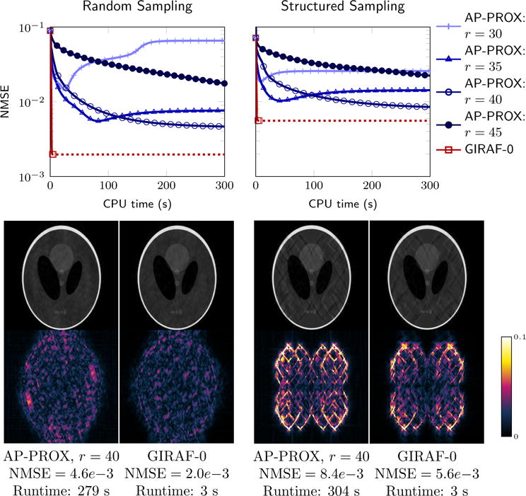
Comparison of GIRAF with LORAKS AP-PROX algorithm. Plotted is the per iteration NMSE against elapsed CPU time in the recovery of synthetic data from the indicated from random Fourier sampling (left) and a structured grid-like Fourier sampling (right) using the C-LORAKS matrix lifting [62]. The AP-PROX algorithm requires a rank estimate r, which needs fine-tuning to obtain the best NMSE. By contrast, the GIRAF algorithm does not require a rank estimate, and in these experiments, converged to a solution with lower NMSE.

2) GIRAF for piecewise constant image recovery

Here we test the GIRAF-0 algorithm for the exact recovery of images belonging to the piecewise constant SLRA model proposed in [9], which uses the gradient weighted matrix lifting described in (9). We adapt the AP, AP-PROX, SVT, SVT+UV, and IRLS-0 algorithms to this setting. To compare computation time among algorithms, we first experiment with recovering simulated piecewise constant images from their undersampled Fourier coefficients. The datasets used in these experiments are shown in Figure 9. In each experiment, we sample uniformly at random in Fourier domain at the specified undersampling factor (USF). Since the simulated Fourier coefficients are noise-free, each algorithm incorporates equality data constraints, as in the formulation (12). To ensure a fair comparison, the algorithms that use a rank estimate (AP, SVT+UV) were passed either the exact rank of the simulated data, which was calculated either using the known bandwidth of the level-set polynomial describing the edge-set of the image (see [9]), or the index for which the normalized singular values were less than 10⁻². The results of these experiments are shown in Table I. We report the CPU time and number of iterations for each algorithm to reach $\text{NMSE}={\Vert \mathit{x}-{\mathit{x}}_0\Vert }^2/{\Vert {\mathit{x}}_0\Vert }^2\le {10}^{-4}$, where x is the reconstruction at the current iterate, and x₀ is the ground truth data. We use the NMSE as a error metric since the competing algorithms solve different cost functions, and cannot be compared on the basis of how well they minimize a common cost function. Observe that for small to medium problem sizes (PWC1, and PWC2), the GIRAF algorithm is competitive or significantly faster than state-of-the-art methods. For the large-scale problems (SL, and BRAIN) the GIRAF algorithm converges orders of magnitude faster than competing algorithms, demonstrating its superior scalability. GIRAF is also successful on all the “hard” problem instances where SVT fails to converge below the set NMSE tolerance.

In Figure 10 we show the results of a similar recovery experiment, but where the Fourier samples are corrupted with noise. We test on the SL dataset with USF = 0.65, adding complex white Gaussian noise to the Fourier samples such that the signal-to-noise ratio (SNR) is approximately 22 dB. Here we test GIRAF against AP-PROX and SVT-UV in their regularized formulations, (16), tuning regularization parameters to obtain the optimal NMSE in each case. In this experiment and subsequent ones we report the time each algorithm took to reach 1% of the final NMSE, where the final NMSE is obtained by running each algorithm until the relative change in NMSE between iterates is less than 10⁻⁶. We observe the GIRAF algorithm shows similar run-time as in the noise-free setting, and converges to a solution with smaller NMSE.

Fig. 10.

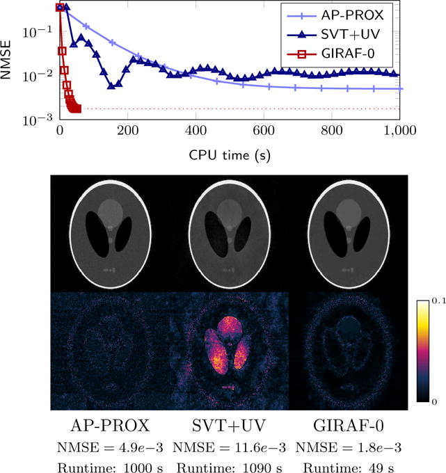
Comparison of GIRAF with competing algorithms for structured low-rank matrix recovery with noisy data using a piecewise constant SLRA model. Plotted is the per iteration NMSE against elapsed CPU time in the recovery of synthetic data from noisy random uniform Fourier samples (USF=0.65, sample SNR=22dB).

3) Application to compressed sensing MRI reconstruction

In Figure 11 we demonstrate the GIRAF algorithm for the recovery of real MRI data from undersampled Fourier data using the gradient weighted lifting scheme. The datasets we experiment on were obtained from a fully sampled four-coil parallel MRI acquisition, compressed into a single virtual coil using an SVD-based technique [63]. We then retrospectively undersample the single virtual coil. To compensate for complex phase in the data, we estimate the phase of the image from very few of its low-pass Fourier samples, and incorporate this into the measurement operator A, as recommended in [1]. To demonstrate the potential benefit of a Fourier domain SLRA approach over standard discrete spatial domain penalties, we compare against a standard total variation (TV) regularized reconstruction, implemented with an efficient ADMM/Split-Bregman approach [64]. We use the GIRAF-0 algorithm with a filter size of 55 × 55. Observe that the GIRAF reconstruction shows nearly a 1dB improvement in SNR = 10 log₁₀(NMSE) over the TV reconstruction. We use a relatively high undersampling factor to illustrate the difference in reconstruction quality over TV; the reconstruction quality may not be appropriate for radiological evaluations. The runtime of GIRAF algorithm on these datasets is roughly 1–2 minutes. While this is slower than a TV reconstruction, which takes roughly 5–10 seconds, it is still substantially faster than previous reported single-coil SLRA-based MRI reconstruction schemes [4], [30]. Moreover, for these experiments we could not compare against the AP-PROX or SVT+UV algorithms because of memory limitations.

Fig. 11.

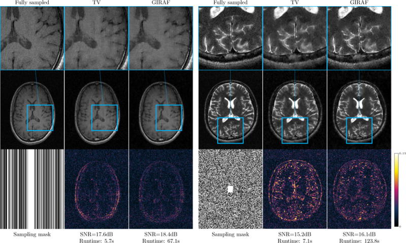
Undersampled MRI reconstruction using GIRAF algorithm with piecewise constant SLRA model. We retrospectively undersample in Fourier domain from variable density random Cartesian lines (left) uniform random sampling mask with a calibration region (right), both with USF=0.50. In each case we show the total variation (TV) regularized recovery and the SLRA recovery using GIRAF. Error images are shown in the bottom row.

One advantage of the GIRAF algorithm is that it scales well with filter size over competing algorithms. We show in Figure 12 that using larger filter sizes directly translates to improved image quality in the case of the gradient weighted lifting, with modest increases in run-time.

Fig. 12.

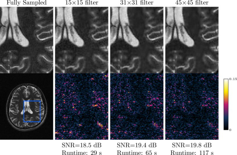
Effect of filter size on reconstruction; zoomed for detail. We reconstruct Fourier data from 20% random variable density samples using the GIRAF-0 algorithm and the gradient weighted lifting scheme. The reconstruction shows a +1dB change in SNR by increasing the filter size from 15 × 15 to 45 × 45, with only a four-fold increase in run-time.

VI. Discussion and conclusion

We introduced the GIRAF algorithm for multi-level Toeplitz/Hankel low-rank matrix recovery problems arising in MRI reconstruction and other imaging applications. The algorithm is based on the IRLS approach for low-rank matrix completion, combined with a novel half-circulant approximation of multi-level Toeplitz matrices. This approximation dramatically reduces the computational complexity and memory demands of the direct IRLS algorithm for large problem sizes. Due to the monotonicity of the Schatten-p regularizer with respect to the half-circulant approximation, we show it suffices to regularize the approximated matrix, rather than the original multi-level Toeplitz matrix. Compared to previous approaches the GIRAF algorithm is an order of magnitude faster on several realistic problem instances. This is because in the GIRAF algorithm performs most of its computations in the original “un-lifted” problem domain with FFTs, rather than in the “lifted” matrix domain. An important feature of the GIRAF algorithm is that it can accommodate larger filters required by more sophisticated image priors, such as the off-the-grid piecewise constant image model proposed in [9]. This enables SLRA/annihilating filter approaches for a much wider class of imaging problems, including realistic large-scale multidimensional datasets, such as those encountered in multi-dimensional MRI reconstruction tasks.

Unlike some previous approaches, the GIRAF algorithm does not require strict low-rank approximations, nor does it require an estimate of the underlying rank or model-order. Arguably the optimal selection of the ε₀ smoothing parameter used in the GIRAF algorithm implicitly performs model-order selection. However, we propose a method to automatically set this parameter based on spectral properties of the initialization to the algorithm. Similar strategies could be used for other algorithms that require a rank estimate to reduce their dependence on the rank.

The multi-level Toeplitz matrix lifting model considered in this work may seem narrow in application, but in fact a variety of existing SLRA models belong to this class, giving the GIRAF algorithm fairly wide applicability. Single-level Toeplitz/Hankel matrix liftings form the foundation for several modern approaches in spectral estimation [58], direction-of-arrival estimation [65], and system identification [44]. Multi-level Toeplitz/Hankel matrix liftings have been used for multi-dimensional spectral estimation [3], [66], and video inpainting [30], [67]. Of particular interest is the application of the framework to super-resolution microscopy [68], which is of high significance in biological imaging. SLRA methods have been seen to be very promising in this context [29], offering more accurate localizations than state-of-the-art methods; the GIRAF algorithm could potentially enable the extension of these methods to recover the whole image rather than small patches, due to its low memory demand. Similarly, most of the SLRA models proposed for MRI reconstruction have a block multi-level Toeplitz/Hankel matrix structure. For example, the SAKE framework for parallel MRI reconstruction [2] considers a matrix lifting with a horizontal block structure, where each block is a multi-level Hankel matrix. Similarly, the matrix liftings considered in the LORAKS [4], [10] and ALOHA [6] frameworks have block multi-level Toeplitz/Hankel structure. In this work we restricted our attention to matrix liftings having a vertical block structure. While our current algorithm is not readily applicable to these settings, the GIRAF framework could also potentially be generalized to more general block-rectangular liftings, such as those used parallel MRI context [2], [10]; we save this as a topic for future work.

Finally, the approximation intrinsic to the GIRAF approach means that the algorithm might not be appropriate for all SLRA problems. For instance, if the rank of the lifted matrix is expected to be very small and is known in advance, singular value thresholding or alternating projection algorithms may be more efficient or more accurate. However, for the large-scale SLRA problems encountered in imaging, where the rank of the lifted matrix is typically unknown and possibly large, our numerical experiments show the GIRAF approach represents a desirable trade-off between accuracy and runtime versus other state-of-the-art algorithms.

Appendix Majorization-minimization formulation of IRLS-p algorithm

Majorization-minimization (MM) algorithms iteratively minimize a given cost function by minimizing a surrogate cost function that upper bounds the original at each iteration [49]. More precisely, if f(x) is any real-valued cost function on a domain Ω, a function g(x; x₀) defined on Ω × Ω is said to majorize f(x) at the fixed value x₀ ∈ Ω if

$$g\left(\mathit{x};{\mathit{x}}_0\right)\ge f\left(\mathit{x}\right),\text{for}\text{all}\mathit{x}\in \mathrm{\Omega }$$ (49)

$$g\left({\mathit{x}}_0;{\mathit{x}}_0\right)=f\left({\mathit{x}}_0\right)$$ (50)

If (49) and (50) hold for all x₀ ∈ Ω then g is called a majorizer for f. An MM algorithm finds a minimizer for f by sequentially solving for the iterates

$${\mathit{x}}^{\left(n+1\right)}=\underset{\mathit{x}\in \mathrm{\Omega }}{\arg min}g\left(\mathit{x};{\mathit{x}}^{(n)}\right).$$ (51)

Using properties (49) and (50) it is easy to show the cost function f must monotonically decrease at each iteration. Furthermore, if f is strongly convex, the iterates x⁽ⁿ⁾ are guaranteed to converge to the unique global minimizer of f; when convexity is violated, the iterates are still guaranteed to converge to a stationary point [69].

We now construct a majorizer for the Schatten p-norm ${\Vert \cdot \Vert }_p^p$, including values of p ∈ [0, 1) where the penalty is non-convex. Let $H_{+}^N$ denote the space of Hermitian positive semidefinite N × N matrices and $H_{++}^N$ the space of Hermitian positive definite N × N matrices. If f: [0, ∞)→ ℝ is any scalar function, and $\mathit{Y}\in H_{+}^N$, we can define f(Y) by $f\left(\mathit{Y}\right):={\displaystyle {\sum }_{i}f\left({\lambda }_i\right){\mathit{P}}_i}$ where Y Has the spectral decomposition $\mathit{Y}={\displaystyle {\sum }_i{\lambda }_i{\mathit{P}}_i}$, i.e., λ_i ≥ 0 are the eigenvalues of Y and P_i are the orthogonal projectors onto the corresponding eigenspaces. In particular, the qth power Y^q, q ∈ (0, 1], of any $\mathit{Y}\in H_{+}^N$ is defined as

$${\mathit{Y}}^q={\displaystyle \sum _i{\lambda }_i^q{\mathit{P}}_i}.$$ (52)

Likewise, for any $\mathit{Y}\in H_{++}^N$, log(Y) is defined as

$$\log \left(\mathit{Y}\right)={\displaystyle \sum _i\log \left({\lambda }_i\right){\mathit{P}}_i}$$ (53)

Our majorizer is derived from the following trace inequalities:

Proposition 1

If ${\mathit{Y}}_0\in H_{++}^N$ then for all $\mathit{Y}\in H_{+}^N$ we have

$$Tr\left[{\mathit{Y}}^q\right]\le \mathit{Tr}\left[{\mathit{Y}}_0^q+q{\mathit{Y}}_0^{q-1}\left(\mathit{Y}-{\mathit{Y}}_0\right)\right]$$ (54)

for all q ∈ (0, 1]. If additionally $\mathit{Y}\in H_{++}^N$, then

$$Tr\left[\log \left(\mathit{Y}\right)\right]\le Tr\left[\log \left({\mathit{Y}}_0\right)+{\left({\mathit{Y}}_0\right)}^{-1}\left(\mathit{Y}-{\mathit{Y}}_0\right)\right]$$ (55)

Proof

These are special cases of Klein’s inequality (see, e.g., Proposition 2.5.2 in [70]), which states that for any concave function f: [0, ∞) → ℝ differentiable on (0, ∞), and any $\mathit{Y}\in H_{+}^N$, ${\mathit{Y}}_0\in H_{++}^N$ we have

$$Tr\left[f\left(\mathit{Y}\right)-f\left({\mathit{Y}}_0\right)-f^{\prime }\left({\mathit{Y}}_0\right)\left(\mathit{Y}-{\mathit{Y}}_0\right)\right]\le 0$$ (56)

where f(X):= Σ_if(λ_i)P_i when X has the spectral decomposition X = Σ_iλ_iP_i. Choosing f(t) = t^q and f(t) = log(t) gives the desired inequalities. □

Let X, ${\mathit{X}}_0\in {ℂ}^{M\times N}$ where X is arbitrary and X₀ has no zero singular values. Substituting $\mathit{Y}={\mathit{X}}^{\ast }\mathit{X}\in H_{+}^N$, ${\mathit{Y}}_0={\mathit{X}}_0^{\ast }{\mathit{X}}_0\in H_{++}^N$, and q = p/2 into (54), it follows that the function

$$g_p\left(\mathit{X};{\mathit{X}}_0\right)=\frac{1}{2}Tr[{\left({\mathit{X}}_0^H{\mathit{X}}_0\right)}^{\frac{p}{2}}+\frac{p}{2}{\left({\mathit{X}}_0^H{\mathit{X}}_0\right)}^{\frac{p}{2}-1}\left({\mathit{X}}^H\mathit{X}-{\mathit{X}}_0^H{\mathit{X}}_0\right)]=\frac{1}{2}Tr[{\left({\mathit{X}}_0^H{\mathit{X}}_0\right)}^{\frac{p}{2}-1}{\mathit{X}}^H\mathit{X}]+C\left({\mathit{X}}_0\right)$$ (57)

$$=\frac{1}{2}{\Vert \mathit{X}\sqrt{{\left({\mathit{X}}_0^H{\mathit{X}}_0\right)}^{\frac{p}{2}-1}}\Vert }_F^2+C\left({\mathit{X}}_0\right),$$ (58)

where C(X₀) is a term depending only on X₀, satisfies the majorization relations

$$g_p\left(\mathit{X};{\mathit{X}}_0\right)\ge {\Vert \mathit{X}\Vert }_p^p,\text{for}\text{all}\mathit{X}\in {ℂ}^{M\times N}$$ (59)

$$g_p\left(\mathit{X};{\mathit{X}}_0\right)={\Vert {\mathit{X}}_0\Vert }_p^p$$ (60)

for all p ∈ (0, 1]. A similar argument using inequality (55) shows that (59) and (60) can be extended to hold for the p = 0 case, with the majorizer g₀(X; X₀) defined by (58) with p = 0. Finally, substituting $\mathit{X}=\mathcal{T}\left(\mathit{x}\right)$ gives the following MM scheme for minimizing the Schatten-p penalty:

$${\mathit{x}}^{\left(n\right)}=\underset{\mathit{x}}{\arg min}\frac{1}{2}{\Vert \mathit{A}\mathit{x}-\mathit{b}\Vert }_2^2+\frac{\lambda }{2}{\Vert \mathcal{T}\left(\mathit{x}\right)\sqrt{{\mathit{H}}_n}\Vert }_F^2$$ (61)

where H_n is determined by the previous iterate x⁽ⁿ⁻¹⁾ according to

$${\mathit{H}}_n={[\mathcal{T}{\left({\mathit{x}}^{\left(n-1\right)}\right)}^{\ast }\mathcal{T}\left({\mathit{x}}^{\left(n-1\right)}\right)]}^{\frac{p}{2}-1},$$ (62)

To ensure the matrix in (62) is invertible, we can introduce a smoothing parameter ε_n and update instead

$${\mathit{H}}_n={[\mathcal{T}{\left({\mathit{x}}^{\left(n-1\right)}\right)}^{\ast }\mathcal{T}\left({\mathit{x}}^{\left(n-1\right)}\right)+{\epsilon }_n\mathit{I}]}^{\frac{p}{2}-1},$$ (63)

where we take ε_n → 0 as n → ∞. This gives the IRLS-p algorithm as shown in Algorithm 1.

References

- 1.Lustig M, Donoho D, Pauly JM. Sparse MRI: The application of compressed sensing for rapid MR imaging. Magnetic Resonance in Medicine. 2007;58(6):1182–1195. doi: 10.1002/mrm.21391. [DOI] [PubMed] [Google Scholar]
- 2.Shin PJ, Larson PE, Ohliger MA, Elad M, Pauly JM, Vigneron DB, Lustig M. Calibrationless parallel imaging reconstruction based on structured low-rank matrix completion. Magnetic Resonance in Medicine. 2014;72(4):959–970. doi: 10.1002/mrm.24997. [DOI] [PMC free article] [PubMed] [Google Scholar]
- 3.Chen Y, Chi Y. Robust spectral compressed sensing via structured matrix completion. Information Theory, IEEE Transactions on. 2014;60(10):6576–6601. [Google Scholar]
- 4.Haldar JP. Low-rank modeling of local k-space neighborhoods (LORAKS) for constrained MRI. IEEE Transactions on Medical Imaging. 2014;33(3):668–681. doi: 10.1109/TMI.2013.2293974. [DOI] [PMC free article] [PubMed] [Google Scholar]
- 5.Haldar JP. Low-rank modeling of local k-space neighborhoods: from phase and support constraints to structured sparsity. SPIE Optical Engineering+ Applications International Society for Optics and Photonics. 2015:959710–959710. [Google Scholar]
- 6.Jin KH, Lee D, Ye JC. A general framework for compressed sensing and parallel MRI using annihilating filter based low-rank Hankel matrix. IEEE Transactions on Computational Imaging. 2016;2(4):480–495. [Google Scholar]
- 7.Jin KH. A novel k-space annihilating filter method for unification between compressed sensing and parallel MRI. International Symposium on Biomedical Imaging (ISBI) 2015 Apr; [Google Scholar]
- 8.Ongie G, Jacob M. Sampling Theory and Applications (SampTA) Washington DC: 2015. Recovery of piecewise smooth images from few Fourier samples. [Google Scholar]
- 9.Ongie G, Jacob M. Off-the-grid recovery of piecewise constant images from few Fourier samples. SIAM Journal on Imaging Science. 2016 doi: 10.1137/15M1042280. vol To appear. pre-print available online: http://arxiv.org/abs/1510.00384. [DOI] [PMC free article] [PubMed]
- 10.Haldar JP, Zhuo J. P-LORAKS: Low-rank modeling of local k-space neighborhoods with parallel imaging data. Magnetic resonance in medicine. 2015 doi: 10.1002/mrm.25717. [DOI] [PMC free article] [PubMed] [Google Scholar]
- 11.Kim TH, Setsompop K, Haldar JP. LORAKS makes better SENSE: Phase-constrained partial fourier SENSE reconstruction without phase calibration. Magnetic Resonance in Medicine. 2016 doi: 10.1002/mrm.26182. [DOI] [PMC free article] [PubMed] [Google Scholar]
- 12.Griswold MA, Jakob PM, Heidemann RM, Nittka M, Jellus V, Wang J, Kiefer B, Haase A. Generalized autocalibrating partially parallel acquisitions (GRAPPA) Magnetic resonance in medicine. 2002;47(6):1202–1210. doi: 10.1002/mrm.10171. [DOI] [PubMed] [Google Scholar]
- 13.Morrison RL, Jacob M, Do MN. Biomedical Imaging: From Nano to Macro, 2007 ISBI 2007 4th IEEE International Symposium on. IEEE; 2007. Multichannel estimation of coil sensitivities in parallel MRI; pp. 117–120. [Google Scholar]
- 14.Lustig M, Pauly JM. SPIRiT: Iterative self-consistent parallel imaging reconstruction from arbitrary k-space. Magnetic resonance in medicine. 2010;64(2):457–471. doi: 10.1002/mrm.22428. [DOI] [PMC free article] [PubMed] [Google Scholar]
- 15.Zhang J, Liu C, Moseley ME. Parallel reconstruction using null operations. Magnetic Resonance in Medicine. 2011;66(5):1241–1253. doi: 10.1002/mrm.22899. [DOI] [PMC free article] [PubMed] [Google Scholar]
- 16.Mani M, Jacob M, Kelley D, Magnotta V. Multi-shot multi-channel diffusion data recovery using structured low-rank matrix completion. 2016 doi: 10.1002/mrm.26382. arXiv preprint arXiv:1602.07274. [DOI] [PMC free article] [PubMed] [Google Scholar]
- 17.Lee J, Jin KH, Ye JC. Reference-free single-pass EPI Nyquist ghost correction using annihilating filter-based low rank Hankel matrix (ALOHA) Magnetic Resonance in Medicine. 2016 doi: 10.1002/mrm.26077. [DOI] [PubMed] [Google Scholar]
- 18.Ye JC, Kim JM, Jin KH, Lee K. Compressive sampling using annihilating filter-based low-rank interpolation. IEEE Transactions on Information Theory. 2016 [Google Scholar]
- 19.Ongie G, Biswas S, Jacob M. Image Processing (ICIP), 2016 IEEE International Conference on. IEEE; 2016. Structured low-rank recovery of piecewise constant signals with performance guarantees; pp. 963–967. [DOI] [PMC free article] [PubMed] [Google Scholar]
- 20.Fornasier M, Rauhut H, Ward R. Low-rank matrix recovery via iteratively reweighted least squares minimization. SIAM Journal on Optimization. 2011;21(4):1614–1640. [Google Scholar]
- 21.Mohan K, Fazel M. Iterative reweighted algorithms for matrix rank minimization. The Journal of Machine Learning Research. 2012;13(1):3441–3473. [Google Scholar]
- 22.Lai MJ, Xu Y, Yin W. Improved iteratively reweighted least squares for unconstrained smoothed ℓq minimization. SIAM Journal on Numerical Analysis. 2013;51(2):927–957. [Google Scholar]
- 23.Xie Y, Gu S, Liu Y, Zuo W, Zhang W, Zhang L. Weighted Schatten p-norm minimization for image denoising and background subtraction. IEEE transactions on image processing. 2016;25(10):4842–4857. [Google Scholar]
- 24.Hintermuller M, Valkonen T, Wu T. Limiting aspects of non-convex TVphi models. SIAM J Imaging Sciences. 2015:2581–2621. [Google Scholar]
- 25.Erway JB, Plemmons RJ, Adhikari L, Marcia RF. Information Theory and Its Applications (ISITA), 2016 International Symposium on. IEEE; 2016. Trust-region methods for nonconvex sparse recovery optimization; pp. 275–279. [Google Scholar]
- 26.Chu MT, Funderlic RE, Plemmons RJ. Structured low rank approximation. Linear algebra and its applications. 2003;366:157–172. [Google Scholar]
- 27.Markovsky I. Structured low-rank approximation and its applications. Automatica. 2008;44(4):891–909. [Google Scholar]
- 28.Ongie G, Jacob M. Super-resolution MRI using finite rate of innovation curves. IEEE International Symposium on Biomedical Imaging: ISBI 2015. 2015 [Google Scholar]
- 29.Min J, Carlini L, Unser M, Manley S, Ye JC. Fast live cell imaging at nanometer scale using annihilating filter based low rank Hankel matrix approach. SPIE Optical Engineering+ Applications International Society for Optics and Photonics. 2015 95 970V–95 970V. [Google Scholar]
- 30.Jin KH, Ye JC. Annihilating filter-based low-rank hankel matrix approach for image inpainting. Image Processing, IEEE Transactions on. 2015;24(11):3498–3511. doi: 10.1109/TIP.2015.2446943. [DOI] [PubMed] [Google Scholar]
- 31.De Prony BGR. Essai experimental et analytique: sur les lois de la dilatabilité de fluides élastique et sur celles de la force expansive de la vapeur de l’alkool,a différentes températures. Journal de l’école polytechnique. 1795;1(22):24–76. [Google Scholar]
- 32.Schmidt RO. Multiple emitter location and signal parameter estimation. Antennas and Propagation, IEEE Transactions on. 1986;34(3):276–280. [Google Scholar]
- 33.Paulraj A, Roy R, Kailath T. Circuits, Systems and Computers, 1985 Nineteeth Asilomar Conference on. IEEE; 1985. Estimation of signal parameters via rotational invariance techniques-esprit; pp. 83–89. [Google Scholar]
- 34.Hua Y, Sarkar TK. Matrix pencil method for estimating parameters of exponentially damped/undamped sinusoids in noise. IEEE Transactions on Acoustics, Speech, and Signal Processing. 1990;38(5):814–824. [Google Scholar]
- 35.Stoica P, Moses RL. Introduction to spectral analysis Prentice hall Upper Saddle River, NJ. 1997;1 [Google Scholar]
- 36.Strichartz RS. A guide to distribution theory and Fourier transforms. World Scientific; 2003. [Google Scholar]
- 37.Pan H, Blu T, Dragotti PL. Sampling curves with finite rate of innovation. Signal Processing, IEEE Transactions on. 2014;62(2) [Google Scholar]
- 38.Liang ZP, Haacke EM, Thomas CW. High-resolution inversion of finite fourier transform data through a localised polynomial approximation. Inverse Problems. 1989;5(5):831. [Google Scholar]
- 39.Haacke EM, Liang ZP, Izen SH. Constrained reconstruction: A superresolution, optimal signal-to-noise alternative to the fourier transform in magnetic resonance imaging. Medical Physics. 1989;16(3):388–397. doi: 10.1118/1.596427. [DOI] [PubMed] [Google Scholar]
- 40.Haacke E, Liang ZP, Izen S. Superresolution reconstruction through object modeling and parameter estimation. Acoustics, Speech and Signal Processing, IEEE Transactions on. 1989 Apr;37(4):592–595. [Google Scholar]
- 41.Haacke EM, Liang ZP, Boada FE. Image reconstruction using POCS, model constraints, and linear prediction theory for the removal of phase, motion, and gibbs artifacts in magnetic resonance and ultrasound imaging. Optical Engineering. 1990;29(5):555–566. [Google Scholar]
- 42.Candès EJ, Recht B. Exact matrix completion via convex optimization. Foundations of Computational Mathematics. 2009;9(6):717–772. [Google Scholar]
- 43.Cai JF, Liu S, Xu W. A fast algorithm for reconstruction of spectrally sparse signals in super-resolution. Proc SPIE. 2015;9597:95 970A–95 970A-7. [Google Scholar]
- 44.Fazel M, Pong TK, Sun D, Tseng P. Hankel matrix rank minimization with applications to system identification and realization. SIAM Journal on Matrix Analysis and Applications. 2013;34(3):946–977. [Google Scholar]
- 45.Markovsky I, Usevich K. Structured low-rank approximation with missing data. SIAM Journal on Matrix Analysis and Applications. 2013;34(2):814–830. [Google Scholar]
- 46.Voevodin VV, Tyrtyshnikov EE. Numerical methods for solving problems with toeplitz matrices. USSR Computational Mathematics and Mathematical Physics. 1981;21(3):1–14. [Google Scholar]
- 47.Vetterli M, Marziliano P, Blu T. Sampling signals with finite rate of innovation. Signal Processing, IEEE Transactions on. 2002;50(6):1417–1428. [Google Scholar]
- 48.Shang F, Liu Y, Cheng J. Tractable and scalable schatten quasi-norm approximations for rank minimization. Proc 19th Int Conf Artif Intell Statist. 2016:620–629. [Google Scholar]
- 49.Hunter DR, Lange K. A tutorial on MM algorithms. The American Statistician. 2004;58(1):30–37. [Google Scholar]
- 50.Larsen RM. Lanczos bidiagonalization with partial reorthogonalization. DAIMI Report Series. 1998;27(537) [Google Scholar]
- 51.Halko N, Martinsson PG, Tropp JA. Finding structure with randomness: Probabilistic algorithms for constructing approximate matrix decompositions. SIAM review. 2011;53(2):217–288. [Google Scholar]
- 52.Paige CC, Saunders MA. LSQR: An algorithm for sparse linear equations and sparse least squares. ACM Transactions on Mathematical Software (TOMS) 1982;8(1):43–71. [Google Scholar]
- 53.Horn RA, Johnson CR. Topics in matrix analysis. Cambridge Univ Press; Cambridge etc: 1991. [Google Scholar]
- 54.Boyd S, Parikh N, Chu E, Peleato B, Eckstein J. Distributed optimization and statistical learning via the alternating direction method of multipliers. Foundations and Trends® in Machine Learning. 2011;3(1):1–122. [Google Scholar]
- 55.Eckstein J, Bertsekas DP. On the Douglas—Rachford splitting method and the proximal point algorithm for maximal monotone operators. Mathematical Programming. 1992;55(1):293–318. [Google Scholar]
- 56.Cadzow JA. Signal enhancement-a composite property mapping algorithm. Acoustics, Speech and Signal Processing, IEEE Transactions on. 1988;36(1):49–62. [Google Scholar]
- 57.Blu T, Dragotti PL, Vetterli M, Marziliano P, Coulot L. Sparse sampling of signal innovations. Signal Processing Magazine, IEEE. 2008;25(2):31–40. [Google Scholar]
- 58.Condat L, Hirabayashi A. Cadzow denoising upgraded: A new projection method for the recovery of Dirac pulses from noisy linear measurements. Sampling Theory in Signal and Image Processing. 2015;14(1):17. [Google Scholar]
- 59.Kim TH, Haldar JP. International Symposium on Biomedical Imaging (ISBI) IEEE; 2015. SMS-LORAKS: Calibrationless simultaneous multislice MRI using low-rank matrix modeling; pp. 323–326. [Google Scholar]
- 60.Cai J, Osher S. Fast singular value thresholding without singular value decomposition. UCLA CAM Report. 2010;5 [Google Scholar]
- 61.Signoretto M, Cevher V, Suykens JA. IEEE Conference on Decision and Control. 2013. An SVD-free approach to a class of structured low rank matrix optimization problems with application to system identification. (no EPFL-CONF-184990). [Google Scholar]
- 62.Haldar JP. Low-rank modeling of local k-space neighborhoods (LORAKS): Implementation and examples for reproducible research. Technical Report USC-SIPI-414. 2014 [Google Scholar]
- 63.Zhang T, Pauly JM, Vasanawala SS, Lustig M. Coil compression for accelerated imaging with cartesian sampling. Magnetic Resonance in Medicine. 2013;69(2):571–582. doi: 10.1002/mrm.24267. [DOI] [PMC free article] [PubMed] [Google Scholar]
- 64.Goldstein T, Osher S. The split Bregman method for L1-regularized problems. SIAM journal on Imaging Sciences. 2009;2(2):323–343. [Google Scholar]
- 65.Pal P, Vaidyanathan P. A grid-less approach to underdetermined direction of arrival estimation via low rank matrix denoising. Signal Processing Letters, IEEE. 2014;21(6):737–741. [Google Scholar]
- 66.Condat L, Boulanger J, Pustelnik N, Sahnoun S, Sengmanivong L. Biomedical Imaging (ISBI), 2014 IEEE 11th International Symposium on. IEEE; 2014. A 2-D spectral analysis method to estimate the modulation parameters in structured illumination microscopy; pp. 604–607. [Google Scholar]
- 67.Ding T, Sznaier M, Camps O, et al. Computer Vision, 2007 ICCV 2007 IEEE 11th International Conference on. IEEE; 2007. A rank minimization approach to video inpainting; pp. 1–8. [Google Scholar]
- 68.Sage D, Kirshner H, Pengo T, Stuurman N, Min J, Manley S, Unser M. Quantitative evaluation of software packages for single-molecule localization microscopy. Nature methods. 2015;12(8):717–724. doi: 10.1038/nmeth.3442. [DOI] [PubMed] [Google Scholar]
- 69.Jacobson MW, Fessler JA. An expanded theoretical treatment of iteration-dependent majorize-minimize algorithms. IEEE Transactions on Image Processing. 2007;16(10):2411–2422. doi: 10.1109/tip.2007.904387. [DOI] [PMC free article] [PubMed] [Google Scholar]
- 70.Ruelle D. Statistical Mechanics: Rigorous Results. 2nd. World Scientific; 1999. [Google Scholar]
Associated Data
This section collects any data citations, data availability statements, or supplementary materials included in this article.