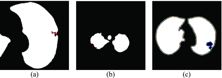
Abstract
Objective: chest computed tomography (CT) images and their quantitative analyses have become increasingly important for a variety of purposes, including lung parenchyma density analysis, airway analysis, diaphragm mechanics analysis, and nodule detection for cancer screening. Lung segmentation is an important prerequisite step for automatic image analysis. We propose a novel lung segmentation method to minimize the juxta-pleural nodule issue, a notorious challenge in the applications. Method: we initially used the Chan–Vese (CV) model for active lung contours and adopted a Bayesian approach based on the CV model results, which predicts the lung image based on the segmented lung contour in the previous frame image or neighboring upper frame image. Among the resultant juxta-pleural nodule candidates, false positives were eliminated through concave points detection and circle/ellipse Hough transform. Finally, the lung contour was modified by adding the final nodule candidates to the area of the CV model results. Results: to evaluate the proposed method, we collected chest CT digital imaging and communications in medicine images of 84 anonymous subjects, including 42 subjects with juxta-pleural nodules. There were 16 873 images in total. Among the images, 314 included juxta-pleural nodules. Our method exhibited a disc similarity coefficient of 0.9809, modified hausdorff distance of 0.4806, sensitivity of 0.9785, specificity of 0.9981, accuracy of 0.9964, and juxta-pleural nodule detection rate of 96%. It outperformed existing methods, such as the CV model used alone, the normalized CV model, and the snake algorithm. Clinical impact: the high accuracy with the juxta-pleural nodule detection in the lung segmentation can be beneficial for any computer aided diagnosis system that uses lung segmentation as an initial step.
Keywords: Active contour, lung segmentation, chest CT images, computer aided diagnosis, juxta-pleural nodule
I. Introduction
Pulmonary or chest computed tomography (CT) images have been used for a variety of purposes, such as lung parenchyma density analysis [1], [2], airway analysis [3], [4], diaphragm mechanics analysis [5], [6] and nodule detection for cancer screening [7]. Recently, with the aid of computing technology, it has become feasible to conduct automatic quantitative analyses. In addition, collaboration among engineers, clinicians, and data scientists has led to the development of accurate automated screening programs for clinical use. Lung segmentation, a step required prior to chest CT imaging analysis, is a crucial starting point for all lung-related quantitative analysis. For instance, in pulmonary nodule detection, when lung segmentation fails to correctly define the borders of the lungs, the nodules outside the borders are missed. One study [8] reported that a computer-aided detection system missed 17% of all true nodules due to erroneous lung segmentations. Thus, an algorithm for automatic and accurate lung segmentation is required.
A large amount of research has been carried out on the topic of lung segmentation in chest CT scans. One of the most common conventional techniques for segmenting lung images is a thresholding approach [9]–[12], wherein the natural contrast between the low-density lungs and the surrounding high-density chest wall is used for lung segmentation. This approach segments the lung image by identifying large differences in attenuation between the lung parenchyma and the surrounding tissue. Another conventional approach is region growing-based lung image segmentation, which is a type of pixel-based segmentation involving the selection of initial seed points. This approach examines the neighboring pixels of initial seed points and determines whether these pixels are within the target region [8], [13], [14]. In addition, more advanced imaging processing techniques have been proposed, including the deformable model [15]–[17], pattern classification [18], [19], rolling ball [8], graph cut-based methods [20]–[23] and Atlas-based methods [14], [24]–[26], all of which generated robust and accurate results. However, most methods are still limited in their ability to accurately differentiate the surrounding tissue from juxta-pleural nodules, which are attached to the walls of the lung. In some cases, the nodules have the same intensity values as the surrounding tissue [27]. Thus, juxta-pleural nodule detection is one of the most challenging issues in lung segmentation.
Recently, much effort has been directed at detecting the juxta-pleural detection [28]–[30]. In [28], the juxta-pleural nodule was detected by skin boundary detection followed by rough segmentation of lung contour and pulmonary parenchyma refinement. In [29], the initial lung volume segmentation was performed by CV model. Then, non-nodules candidates such as small blood vessels were filtered out using a multiscale Laplacian-of-Gaussian filtering. In [30], intuitionistic fuzzy energy was incorporated into length regularization term of region-based level set method, which resolved the boundary leakage. The all methods provided accurate detection results with the slice by slice processing. However, the performance was limited in the case of the blurred juxta-pleural nodules, which is an inherent limitation. In our work, based on the spatially sliced images from top to bottom, we exploited a Bayesian approach, which predicts and updates lung contour from previously estimated contour.
We first initially used the Chan–Vese (CV) model for active contours. The CV model is a powerful and flexible method that is able to segment many types of images. This model is based on the Mumford–Shah function [31] for segmentation, which has been used widely in the medical imaging field, especially for the segmentation of the brain, heart, and trachea [32]–[35]. While many segmentation methods rely heavily in some way on edge detection, the CV model ignores edges completely. Instead, the method optimally fits a two-phase piecewise constant model to the given image by implicitly representing segmentation boundary with a level set function. It allows the segmentation to handle topological changes more easily than snake methods or other edge detection methods. It also uses the global image information without depending on gradient, which results in better management of image segmentation problems such as strong noise and edge blurs. In addition, it can be applied to images whose gradients are either significant or insignificant; thus, it is suitable for images whose boundaries are either smooth or discontinuous [36]. The CV model was previously evaluated for lung segmentation and found to outperform conventional methods [32], [33], [37].
Nevertheless, the juxta-pleural nodule issue has yet to be resolved [34]. To address this issue, we adopted a Bayesian approach based on the CV model results, which predicts the lung image based on the segmented lung contours in the previous frame image or neighboring upper frame image. Note that the frames represent sequential chest CT images “slices” from top to bottom. This approach is based on the assumption that the lung contour is slightly and uniformly expanded or contracted over frames, while the juxta-pleural nodules have a consistent appearance regardless of the pattern of lung contour changes. Based on our Bayesian approach, we predicted and updated the lung contour over multiple frames. Then, we extracted the difference image by comparing the results from the Bayesian approach and the CV model. Here, each separated group in the difference image corresponds to a juxta-pleural nodule candidate. Finally, we investigated whether the separated groups in the difference image comprised juxta-pleural nodules or portions of the lung wall using concave point detection and circle/ellipse Hough transform. We evaluated the performance of our proposed method by comparing it with the CV model [29], the normalized and modified CV (NM-CV) method [38], [39], and the snake model [40].
The main contributions of this study are:
-
•
We proposed a Bayesian approach for automatic juxta-pleural nodule identification in the lung segmentation stage from chest CT scans.
-
•
We presented a concave point detection and circle/ellipse Hough transform to minimize false positives.
-
•
We tested our proposed method from 16,873 images (84 subjects). Among the images, 314 images included juxta-plerual nodules.
-
•
We further validated the method from different databases, which included 1,766 images in total. Among the images, 125 included juxta-pleural nodules.
-
•
We presented the extension capability that accurate lung contour segmentation results can be provided from any global contour results by applying to our proposed method framework.
II. Methods
A. Collection of Chest CT Images
In the present study, we evaluated our proposed method using chest CT scans from Wonkwang University Hospital (WKUH). For the clinical data, we collected chest CT digital imaging and communications in medicine (DICOM) images of 84 anonymous subjects, including 42 subjects with juxta-pleural nodules. Each scan included 150 to 215 image frames, and there were 16,873 images in total. Among the images, 314 included juxta-pleural nodules. The images were acquired at WKUH using a multiple detector computed tomography (MDCT) scanner (Somatom Sensation 16, Siemens, Erlangen, Germany; X-ray tube voltage: 100–120 kV; tube current: 80–328 mA; pixel length: 0.56–0.79 mm). The thickness of each slice was 5.0 mm. The WKUH Institutional Review Board approved the collection and analysis of the imaging data. To evaluate the performance of the model, “gold standard” lung contours were obtained from six trained radiologists. Initially, four trained radiologists drew the contours, and another two trained radiologists confirmed them.
B. Global Lung Contour Extraction With the Chan-Vese Model
To segment the lung contour, we first applied the CV model to chest CT images. Let  be a bounded open subset of
  with the boundary
  . In the evolving lung contour
  , as the boundary of an open subset
  of
of  , inside(C) and outside(C) denote the regions
  and
and  , respectively. The energy term
  is based on the CV model defined with the length of the contour
  , area of the region inside
  , and the averages of
  inside
  and outside
  . Accordingly, the energy term
  is defined by
 |
where  ,
,  ,
,  are fixed parameters. Length(C) is the length of the lung contour
  , and Area(inside(C)) is the region inside
  .
.  is the pixel intensity in
  .
.  and
and  are the intensity averages of inside
  and outside C, respectively. The curve
  is then found to minimize the global energy term
  as
as
 |
To find the solution for  , the level set method is used, which replaces the unknown contour
  by the level set function
  , where
  if the point (x,y) is inside C,
  if the point (x,y) is on
  , and
, and  if the point (x,y) is outside C. Then,
  can be rewritten in terms of
  as follows:
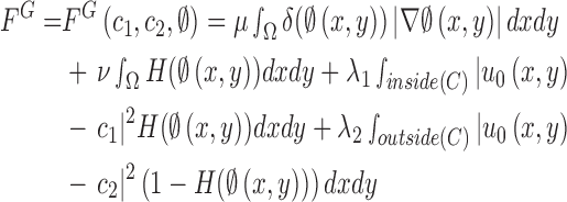 |
where the first term corresponds to  and the second term corresponds to
  . The third and fourth terms correspond to
  and
and  , respectively. The Heaviside function
  is one if
  and zero if
  . Its derivative is the one-dimensional Dirac measure
  . The minimization problem is solved by taking the Euler–Lagrange equations and updating the level set function by the gradient descent method as
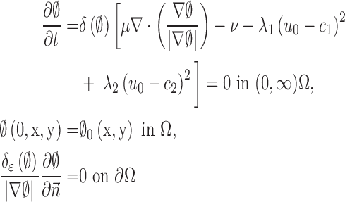 |
where  denotes the exterior normal to the boundary
  , and
, and  denotes the normal derivative of
  at the boundary. Here,
  and
and  are updated at each iteration by
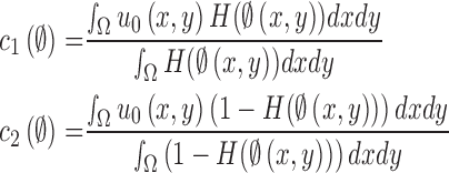 |
For the numerical approximation of the model, the Heaviside function is slightly regularized as
 |
where  . Then,
  and
and  can be replaced by
  and
and  in (4) and (5). For the initialization, we used the checkerboard function in (7) as the level set function, which was used in [41] and [42]. Subsequently,
  and
and  were updated for the initial curve
  .
.
 |
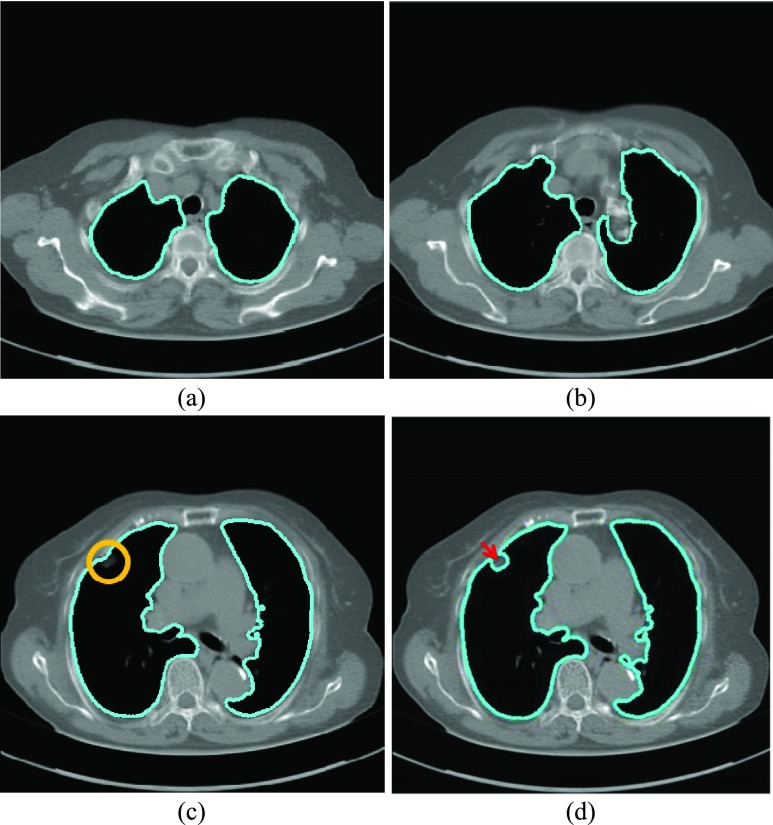
After applying with the CV model on the chest CT image, the nodules or vessels inside the lung parenchyma are also segmented. To separate them from the lung contour, we selected the two longest contours, which correspond to left and right lungs. Fig. 1 shows the CV model-based lung segmentation results from four chest CT images. For the CV model-based lung segmentation, we chose the generally used parameters of  and
and  in [31]. The parameter of
  was chosen by providing the highest accuracy. As
  increases, the results tend to be roughly segmented. All of the parameters were applied to the entire images in this paper.
FIGURE 1.
Lung segmentation results using Chan–Vese (CV) model. (a) and (b) Most lung contours can be accurately segmented. (c) A correct segmentation results in the presence of a juxta-pleural nodule. (d) An incorrect segmentation results in the presence of a juxta-pleural nodule; The incorrect part is pointed by an arrow.
The CV model method provided mostly accurate lung wall segmentation results, as shown in Figs. 1(a) to (c). In particular, in Fig. 1(c), the juxta-pleural nodule is included within the segmented lung contour. On the other hand, in Fig. 1(d), the juxta-pleural nodule is outside the segmented lung contour. This is because the pixel intensities of the juxta-pleural nodule and the adjacent surrounding tissue nearly overlap. The juxta-pleural nodule outside the lung contour ultimately results in missed nodules and incorrect quantitative analyses. In the following subsections, we adopted a Bayesian approach to minimize this juxta-pleural nodule issue.
C. A Bayesian Approach to Juxta-Pleural Nodule Candidate Detection
Given the  successive chest CT image frames, we denote the lung contour state vector of the
  -th image by
  (i.e.
(i.e.  ,
,  ). Note again that the frame represents the spatially sliced image from top to bottom. The state vector
  is assumed to evolve according to the following system model as
 |
where the system transition function  corresponds to the change of lung contour at the
  -th image from the (n-1)-th image. The noise
  is a zero-mean, white-noise sequence independent of past and current states. In the Bayesian approach, the measurement vector is related to the state vector
  via the observation equation. Here, the measurement vector is
  , which is the result from the CV-based method in (4) and (5). Then, the observation equation can be formulated by
 |
where  is the measurement function, and the noise
  is another zero-mean white-noise sequence independent of past and current states and system noise. The initial probability density function (PDF) is
  . The available information at the
  -th frame is the set of measurement vectors, such as
  .
.
The requirement is to construct the PDF of the state vector  , given all the available information of
  , which can be obtained recursively in two stages of prediction and update. Given the required PDF
  available, the prior PDF of the state vector
  can be obtained as
 |
where the first term  is the state evolution based on a Markov model defined by the system transition function
  and
and  . Then,
  can be formulated by
 |
Since  ,
,
 |
where  is the Dirac delta function. At the
  -th frame, a measurement vector
  is available and can be used to update the prior PDF for the posterior PDF via the Bayes rule as
 |
where the normalizing denominator is
 |
The conditional PDF  is defined by the measurement function
  and
and  as
as
 |
In the update stage in (13), the measurement vector  is used to modify the predicted prior PDF in (10) to obtain the required posterior PDF of the state vector
  . Then, the updated posterior PDF is used for the prior PDF at the (n +1)-th frame. The recurrence relations of (10) and (13) constitute the formal solution to the Bayesian recursive estimation problem. More specific prediction and update stages are described in the next subsections.
1). Prediction Stage
Given the contour  , we formed the prior
  in (10) by dilating and contracting
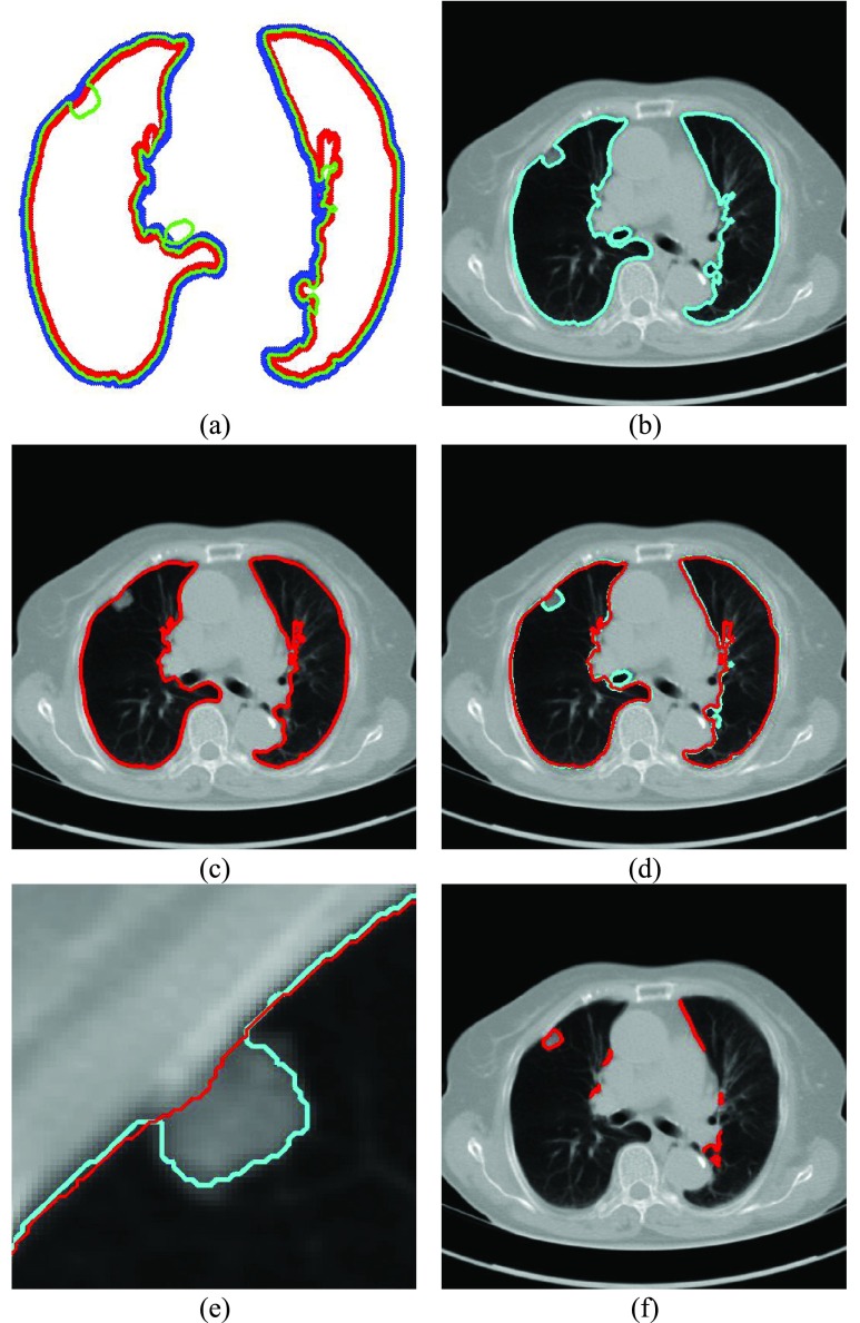
  as shown in Fig. 2(a). The blue areas are dilated curve samples, and the red areas are contracted curve samples. The dilated curves were sampled moving each pixel of
  toward the normal vector, and the contracted curves were sampled moving each of
  toward the opposite normal vector. Each pixel movement for dilation and contraction was from 1 to 5 pixels. In [43], solid nodules smaller than 6 mm do not require routine follow-up in patients since there is a paucity of direct evidence regarding caner probability in small nodules. Thus, we limited the scope to identify the Juxta-pleural nodules smaller than 3mm. Note that the 5 pixel length corresponds to approximately 3mm in the images. Thus, the number of pixels needs to be adjusted according to each different image resolution. The total 10 curve samples represent the prior
  with the system transition function
  considering dilation and contraction at the
  -th frame from the (n-1)-th frame. Here, we ignore the noise
  . We denote the predicted curve samples by
  .
.
FIGURE 2.
(a) Curve samples by  for dilation (blue) and contraction (red) from
  (b) global contour
  (c) contour sample
  providing the highest correlation value between
  and each curve from
  , (d) the overlapped contours of
  and
and  , (e) enlarged and highlighted juxta-pleural nodule area, and (f) the resultant juxta-pleural nodule candidates.
2). Update Stage
Given the measurement vector  obtained from the CV-based method in (4) and (5), we evaluated the likelihood of each contour sample
  to find the best-fitted prediction curve with
  since the lung evolution degree in dilatation or contraction is not exactly known. Hence, we found the best-fitted prediction curve by evaluating the cross-correlation. We first calculated the cross-correlation between
  and each
  , and found that the updated contour sample
  provided the highest correlation values for the left and right lungs. Fig. 2(b) shows the CV model-based contour
  , and Fig. 2(c) shows the resultant updated contour sample
  . Note that the area inside
  does not include the nodule, while the area inside
  does include the nodule. Fig. 2(d) shows the overlapping contours of
  and
and  . For better visualization, we enlarged and highlighted the juxta-pleural nodule area as shown in Fig. 2(e). In the next step, we obtained the difference image between the results from the Bayesian approach and the CV model by finding the segments that were simultaneously outside the contour
  and inside the contour
  . The separated segments are the juxta-pleural nodule candidates. Fig. 2(f) shows the resultant nodule candidates. Then, the lung contour can be modified by adding the nodule candidates to the area of
  , which may form the lung contour
  .
.
D. Elimination of False Positives
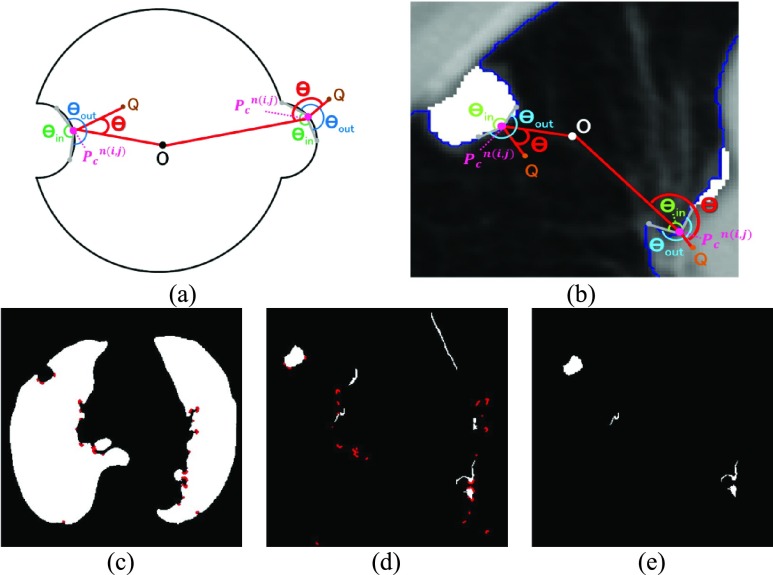
For classifying the nodule candidates as true nodules or false positives, we first investigated whether each candidate contour included any concave point from the center point of  . Let us denote the set of contour points of each nodule candidate by
 |
where  is the total number of nodule candidates and
  is the total number of contour points for the i- th nodule candidate. We calculated the included angle
  , and declared the point
  to be a concave point if the angle was less than 90°, as illustrated in Fig. 3(a). To calculate the angle
  , we first determined the directions of clockwise and counterclockwise rotation with
  and found the fifth points next to
  in each direction. Subsequently, we drew the two lines by connecting each of two points to
  . We denote the resultant angles by
  and
and  , where
  and
and  . We additionally drew the line
  dividing
  equally, where point
  is any point in the drawing direction. Fig. 3(b) shows the angle
  computation examples for the concave point declaration based on the results of Fig. 2(f). In the example, the point
  from the nodule candidate (top left) is declared to be a concave point, while the point
  from the false positive (bottom left) is declared to be a non-concave point. Fig. 3(c) shows the detected concave points with red dots on
  . More specifically, Fig. 3(d) shows the detected concave points on the juxta-pleural nodule candidate contours. Finally, only the nodule candidates including concave points remained, as shown in Fig. 3(e).
FIGURE 3.
(a) Calculation of the included angle  , and declaration of the point
  to be a concave point if the angle was less than 90°. (b) Angle
  computation examples for the concave point declaration based on the results of Fig. 2(f). (c) Detected concave points with red dots on
  . (d) Detected concave points on the juxta-pleural nodule candidate contours, and (e) the remaining nodule candidates that included any concave point.
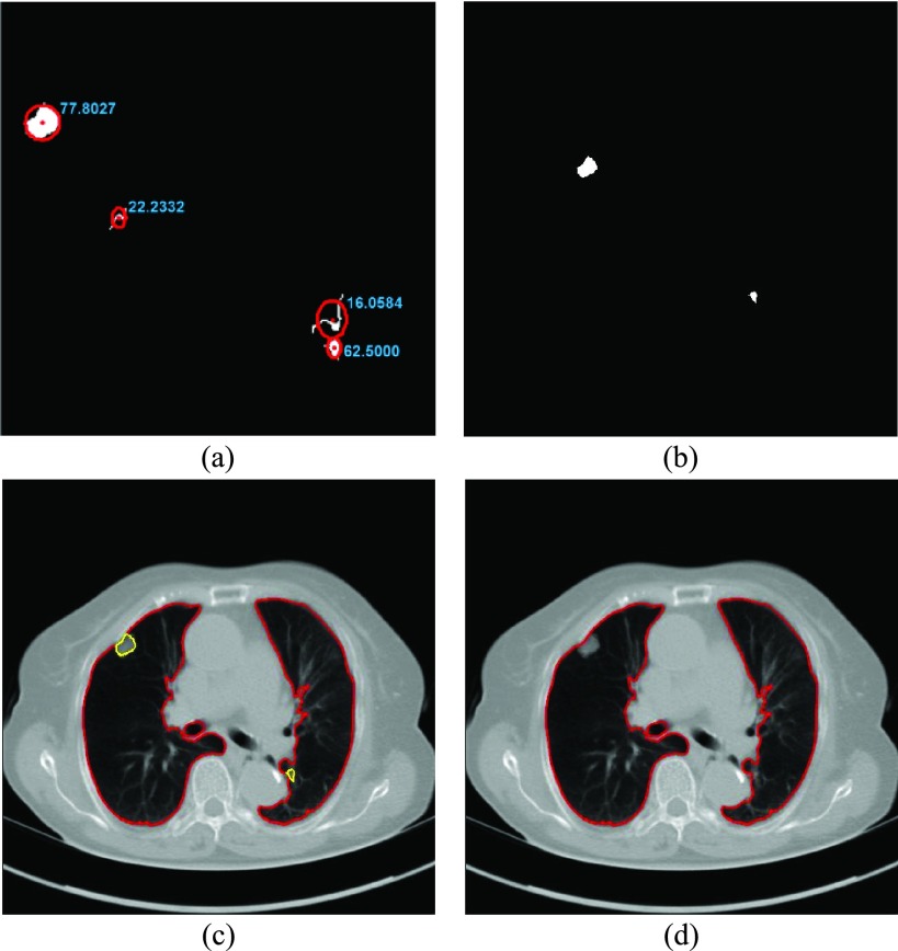
In the last step, we found the circle/ellipse shape segments among the remaining nodule candidates. For circle/ellipse shape detection, we used a circular Hough transform [44]. We computed the circle/ellipse similarity metric  for each segment, and considered only the segments with
  , where
  , which was optimized using the receiver operating characteristic (ROC) curve as detailed in the Results section. Fig. 4(a) shows the similarity metric
  for each remaining segment, and Fig. 4(b) shows the two remaining segments for which where
  was greater than 0.49. Subsequently, the area of the remaining segments (yellow contours) were added to the area inside
 as shown in Fig. 4(c). Then, the lung contour was finally modified by adding the nodule candidates to the area inside
 , which forms the final lung contour, as shown in Fig. 4(d).
FIGURE 4.
(a) Similarity metric  for each remaining segment. (b) Two remaining segments where
  was greater than 0.49. (c) Areas of the remaining segments (yellow contours) were added to the area inside
 . (d) Final lung contours were defined by adding the nodule candidates to the area inside
 .
.
E. Performance Evaluation
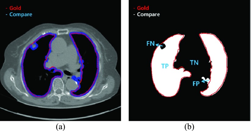
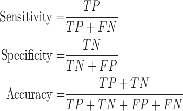
The performance of our proposed method was evaluated using five metrics: the disc similarity coefficient (DSC), modified Hausdorff distance (MHD), sensitivity, specificity, and accuracy. To compute the five metrics, we first calculated the true positive (TP), false positive (FP), true negative (TN), and false negative (FN) values. TP (FP) is the number of positive pixels labeled correctly (incorrectly). TN (FN) is the number of negative pixels labeled correctly (incorrectly). We used an example to quantize the parameters in Fig. 5. In Fig. 5 (a), the gold standard contour (purple) and the estimated contour (blue) are shown, and the corresponding TP, FP, TN, and FN are shown in Fig. 5(b). Each estimated contour was evaluated with each gold standard contour for all images.
FIGURE 5.
(a) Example of the gold standard contour (purple) and estimated contour (blue), and (b) the corresponding true positive (TP), true negative (TN), false positive (FP), and false negative (FN).
Based on the four parameters, the DSC can be calculated as
 |
The DSC is the most commonly used metric for determining the segmentation of false positives and false negatives. It is a statistical approach used to compare the similarity of two data sets, which we used to determine the similarity between the estimated contour and the gold standard. The DSC value ranges between 0 and 1, where 0 means that there is no similarity and 1 means that there is perfect similarity. The MHD measures how far two subsets of a metric space are from each other. It computes the forward and reverse distances and outputs the minimum of both [37]. The other metrics of sensitivity, specificity, and accuracy were calculated as
 |
To evaluate our proposed method, we implemented the CV model [29], the normalized CV (NM-CV) model [38], [39], and the snake algorithm [40], and compared the results with those of our proposed method, based on chest CT images including juxta-pleural nodules ( ) from 42 subjects, and all chest CT images (
 ) from 84 subjects. For the snake algorithm [45], [46], the parameters of length (
 ), curvature (
 ) and smoothing spline (
 ) were used with 0.001, 0 and 100, respectively in [46].
To assess significant differences, we performed one-way analysis of variance (ANOVA) tests with Bonferroni corrections for multiple comparisons ( ) using SPSS ver.18 (SPSS Inc., Chicago, IL, USA).
The Matlab codes of our proposed method is available online both at https://sites.google.com/site/bamilab/sourcecodes/lung-segmentation and https://github.com/HeewonChung92/LungSegmentation.
III. Result
A. ROC Evaluation on 
We computed the circle/ellipse similarity metric  for the remaining nodule candidates (
 ) after the concave point identification based on the all images. To find the optimum threshold value
  , we adjusted the metric
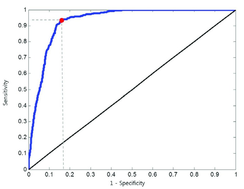
  from 0 to 1 in 0.01 increments, and evaluated the ROC curve. Fig. 6 shows the ROC curve with 1 minus specificity versus sensitivity for
  . For the ROC evaluation, we found the values for TP, TN, FP, and FN, and then calculated the sensitivity, specificity, and accuracy. The best accuracy was found to be 0.9442 with
  , which is also the closest to the upper left corner (Fig. 6).
FIGURE 6.
Receiver operating curve (ROC) curve with 1 minus specificity versus sensitivity in 0.01 increments from 0 to 1.
B. Performance Evaluation and Comparison
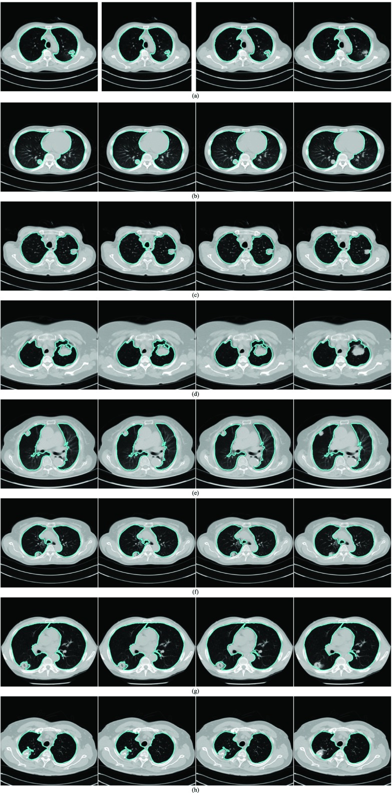
Fig. 7 shows several examples of lung segmentation results using our proposed method (rightmost panels) compared with the CV model (leftmost panels), NM-CV model (second left panels) and snake algorithm (second right panels). The juxta-pleural nodules resulted in incorrect lung segmentation for the CV model, NM-CV model, and snake algorithm. On the other hand, our proposed method correctly segmented the lung, including juxta-pleural nodules within the lung contour area. For example, in Fig. 7(a), the juxta-pleural nodule has similar intensity values compared with the surrounding tissue. The CV model, NM-CV model, and snake algorithm generated contours that excluded the nodules. Similar results can be observed in other conventional approaches, such as thresholding and region growing.
FIGURE 7.
Performance comparison for juxta-pleural nodules: (top left) the CV model, (top right) normalized modified Chan–Vese (NM-CV) model, (bottom left) the snake algorithm, and (bottom right) our proposed method. The performance comparison shown from (a) through (h) includes several juxta-pleural nodule cases.
In our proposed method, the CV model-based result  and the predicted contour sample
  from
from  were evaluated for likelihood based on cross-correlation. Subsequently, the contour sample
  update, followed by concave point detection and Hough transform, could detect the juxta-pleural nodule and modify the results by adding the nodule to the area inside
  , which finally segmented the lung contour
  as shown in the rightmost panel of Fig. 7(a). Figs. 7(b) through (h) also show that our proposed method detected juxta-pleural nodules and correctly segmented lung contours. Therefore, using the combination of the CV model and the Bayesian approach, we achieved accurate lung segmentation and successfully detected juxta-pleural nodules.
To further evaluate our proposed method, we compared the results from the CV model, NM-CV model, the snake algorithm and our proposed method on the CT images that included juxta-pleural nodules ( ). We computed the DSC, MHD, sensitivity, specificity, and accuracy. Fig. 8 shows the distribution of these metrics. The squares at the top and bottom represent the
  and
and  percentiles, respectively. The whiskers at the top and bottom represent the
  and
and  percentiles, respectively, and the circle indicates the median value. Regarding the DSC, our proposed method provided the highest DSC mean value (0.9712), while the CV model, NM-CV model, and the snake algorithm provided mean values of 0.8410, 0.8428, and 0.8198, respectively. Our proposed method provided the lowest MHD mean value (0.4504), while the CV model, NM-CV model, and the snake algorithm provided mean values of 2.1727, 2.1486, and 2.2573, respectively. Our proposed method also provided the highest sensitivity value, 0.9711, while the CV model, NM-CV model, and the snake algorithm provided values of 0.0.7366, 0.7389, and 0.7040, respectively. Regarding accuracy, our proposed method also provided the highest value, 0.9667, while the CV model, NM-CV model and the snake algorithm provided values of 0.8050, 0.8072, and 0.7843, respectively. All of the above results were statistically significant. On the other hand, in our proposed method, the mean specificity value was 0.9637, which was slightly lower than that provided by the other methods. However, the difference was not statistically significant. Furthermore, using our proposed method we could detect 96% of the juxta-pleural nodules and correctly modify the lung contour; conversely, the CV method, NM-CV model, and snake algorithm could detect only 11%, 14%, and 9% of the juxta-pleural nodules, respectively. Table 1 summarizes the results of our comparisons.
FIGURE 8.
Comparison of the four methods: the distribution of the disc similarity coefficient (DSC), modified Hausdorff distance (MHD), sensitivity, specificity, and accuracy. The squares at the top and bottom represent the  and
and  percentiles, respectively. The whiskers at the top and bottom represent the
  and
and  percentiles, respectively, and the circle indicates the median value.
TABLE 1. Comparison of the Performance of the Four Methods on CT Images That Included Juxta-Pleural Nodule ( ). The DSC, MHD, Sensitivity, Specificity, Accuracy, and Juxta-Pleural Nodule Detection Rate Were Evaluated and Compared. Mean, Standard Deviation and Detection Rate are Summarized.
| Method | CV | NMCV | Snake | Proposed method | |
|---|---|---|---|---|---|
| DSC | mean | 0.8410 | 0.8428 | 0.8198 | 0.9712 |
| std | 0.0801 | 0.0782 | 0.0866 | 0.0251 | |
| MHD | mean | 2.1727 | 2.1486 | 2.2573 | 0.4504 |
| std | 1.1679 | 1.1485 | 1.1945 | 0.4433 | |
| Sensitivity | mean | 0.7366 | 0.7389 | 0.7040 | 0.9711 |
| std | 0.1198 | 0.1180 | 0.1243 | 0.0331 | |
| Specificity | mean | 0.9854 | 0.9855 | 0.9983 | 0.9637 |
| std | 0.0208 | 0.0216 | 0.0042 | 0.0716 | |
| Accuracy | mean | 0.8050 | 0.8072 | 0.7843 | 0.9667 |
| std | 0.0972 | 0.0944 | 1.005 | 0.0241 | |
| Detection rate(%) | 11% | 14% | 9% | 96% | |
Finally, we performed our proposed method on all chest CT images ( ). Table 2 summarizes the performance of all models in terms of the DSC, MHD, sensitivity, specificity, and accuracy. Our proposed method provided the highest mean DSC value (0.9709), while the CV model, NM-CV model, and snake algorithm provided mean values of 0.9692, 0.9693, and 0.9684, respectively. Our method provided the lowest mean MHD value (0.5006), compared with 0.5191, 0.5162, and 0.5227 for the CV model, NM-CV model, and snake algorithm, respectively. Our proposed method also provided the highest sensitivity and accuracy values: 0.9585 and 0.9954, respectively. Regarding specificity, the mean specificity value (0.9981) was slightly lower than the other methods by the cost of increased sensitivity. Table 2 summarizes the results of the comparison.
TABLE 2. Results of Comparison of the Four Methods on All Chest CT Images ( ). The DSC, MHD, Sensitivity, Specificity and Accuracy Were Evaluated. The Mean and Standard Deviation are Summarized.
| Method | CV | NMCV | Snake | Proposed method | |
|---|---|---|---|---|---|
| DSC | mean | 0.9692 | 0.9693 | 0.9684 | 0.9709 |
| std | 0.0524 | 0.0513 | 0.0514 | 0.0511 | |
| MHD | mean | 0.5191 | 0.5162 | 0.5227 | 0.5006 |
| std | 0.5978 | 0.5837 | 0.5927 | 0.5771 | |
| Sensitivity | mean | 0.9550 | 0.9554 | 0.9543 | 0.9585 |
| std | 0.0728 | 0.0722 | 0.0746 | 0.0722 | |
| Specificity | mean | 0.9992 | 0.9991 | 0.9993 | 0.9981 |
| std | 0.0015 | 0.0013 | 0.0017 | 0.0012 | |
| Accuracy | mean | 0.9952 | 0.9953 | 0.9951 | 0.9954 |
| std | 0.0129 | 0.0128 | 0.0132 | 0.0129 | |
C. Discussion on Effect of Prediction Order and Limitations
Given the contour  , we formed the prior
  as previously described (10) by dilating and contracting
  . In (10), the term
  is the state evolution based on a Markov model defined by the system transition function
  and
and  . Throughout this paper, we considered the first-order prediction order for the curve samples
  . Here, we may consider higher-order predictions. In second-order or higher predictions, the predicted curve samples
  can be obtained from
  , where
  is the prediction order. It is useful to use the curves
  when
when  is not accurate or when its area inside the contour does not include a juxta-pleural nodule. If the area inside the curve
  does not correctly include a juxta-pleural nodule, the predicted curve samples
  cannot further include the nodule in the final result
  . Furthermore, the successive incorrect
  can continuously and incorrectly evolve in the following frames (i.e. at the n+1, n+2,
  frame). Hence, to avoid this issue, we may consider higher-order predictions by formulating the prior PDF of the state vector
  as
as
 |
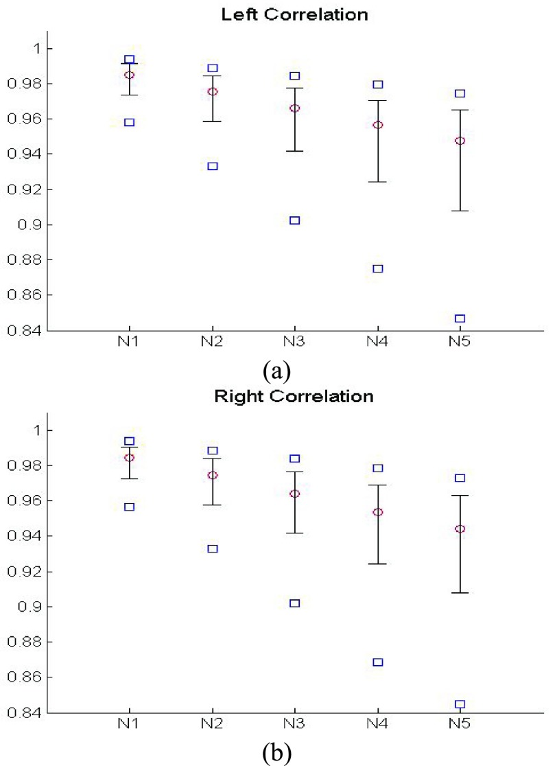
This use of higher-order predictions is based on the assumption that the lung contour does not change rapidly in consecutive frames. Fig. 9 shows the distribution of correlation values between consecutive frames of lung images from the clinical database ( ). It shows that the median correlation value between consecutive lung images at the
  th frame and the (
 )-th frame is 0.9842 for the right lung and 0.9849 for the left lung. Regarding the lung images between the
  th frame and the (
 )-th frame, the correlation median value is slightly lower: 0.9745 for the right lung and 0.9756 for the left lung. However, such second-order or higher predictions may decrease the accuracy of the predicted lung morphology, which may degrade the overall performance in terms of the DSC, MHD, sensitivity, specificity, and accuracy.
FIGURE 9.
Distribution of correlation values between consecutive frame lung images from the clinical database ( ): (a) left lung image correlation and (b) right lung image correlation.
To investigate the effect of the order of predictions, we compared the results of first- and second-order predictions ( and 2). When
  , the prior PDF of the state vector
  can be formulated as
 |
Then, we formed the prior  by dilating and contracting both
  and
and  . The total 20 curve samples represent the prior
  with the system transition function
  considering dilation and contraction at the
  th frame from both the (
 )-th and the (
 )-th frames. We compared the results from
  and 2 on the CT images that included juxta-pleural nodules (
 ), as well as the DSC, MHD, sensitivity, specificity, accuracy, and juxta-pleural nodule detection rate. When
  , the juxta-pleural nodule detection rate increased from 90% to 98%. However, even with the aid of the contour modification from the detected nodule, the DSC, MHD, sensitivity, specificity, and accuracy were all worse than when
  . These results were all statistically significant. The results can be explained by the fact that higher-order prediction decreases the overall accuracy of the predicted lung morphology, which eventually degrades the overall performance in terms of the DSC, MHD, sensitivity, specificity, and accuracy. Table 3 summarizes the results of the comparison.
TABLE 3. Results of the Comparison of  and 2 on CT Images That Included Juxta-Pleural Nodules (
 ). The DSC, MHD, Sensitivity, Specificity, Accuracy, and Juxta-Pleural Nodule Detection Rate Were Evaluated and Compared. Mean, Standard Deviation and Detection Rate are Summarized.
| Method | K = 1 | K = 2 | |
|---|---|---|---|
| DSC | mean | 0.9712 | 0.9025 |
| std | 0.0251 | 0.0887 | |
| MHD | mean | 0.4504 | 1.5042 |
| std | 0.4433 | 1.5099 | |
| Sensitivity | mean | 0.9711 | 0.8850 |
| std | 0.0331 | 0.1358 | |
| Specificity | mean | 0.9637 | 0.9396 |
| std | 0.0716 | 0.0541 | |
| Accuracy | mean | 0.9667 | 0.8741 |
| std | 0.0241 | 0.1089 | |
| Detection rate(%) | 96% | 98% | |
We also compared the results when  or 2 on all chest CT images (
 ). Table 4 summarizes the comparative performance in terms of the DSC, MHD, sensitivity, specificity, and accuracy. As expected, all metrics showed that the results when
  were superior to those when
  . These results were also all statistically significant. Thus, in the future, we need to consider an adaptive approach with variable prediction order that maintains both high segmentation accuracy and high juxta-pleural nodule detection rate.
TABLE 4. Results of the Comparison of  and 2 on all Chest CT Images (
 ). The DSC, MHD, Sensitivity, Specificity, and Accuracy Were Evaluated and Compared. Mean and Standard Deviation are Summarized.
| Method | K = 1 | K = 2 | |
|---|---|---|---|
| DSC | mean | 0.9709 | 0.7323 |
| std | 0.0511 | 0.1152 | |
| MHD | mean | 0.5006 | 1.4270 |
| std | 0.5771 | 0.5586 | |
| Sensitivity | mean | 0.9585 | 0.7755 |
| std | 0.0722 | 0.0697 | |
| Specificity | mean | 0.9981 | 0.7322 |
| std | 0.0012 | 0.1329 | |
| Accuracy | mean | 0.9954 | 0.7321 |
| std | 0.0129 | 0.1517 | |
Given the number of juxta-pleural nodule candidates, the elimination of false positives is a critical step. In our method, irregularly shaped nodule candidates were filtered out through the circle/ellipse detection step. However, the detection of irregularly shaped nodules is crucial in not only automatic lung segmentation but also in automatic nodule detection inside the segmented contour: cancerous nodules are more likely to have irregular shapes, rougher surfaces, and color variations or speckled patterns. Fig. 10 shows the juxta-pleural irregular shape nodules in our clinical database. Unfortunately, those were all filtered out during the circle/ellipse detection step. The missing irregular shape nodule is one of the limitations of our proposed method. Thus, further rigorous research is required for the detection of juxta-pleural nodules without incurring the cost of false positives.
FIGURE 10.
Irregularly shaped juxta-pleural nodules in our clinical database. (a), (b) and (c): The nodules filtered out completely from the circle/ellipse detection step.
Another limitation is that our proposed method cannot identify the nodule if the nodule is first appeared inside the lung parenchyma and becomes adjacent to lung wall in the next slices. This is because the juxta-pleural nodule presents largely beyond our predicted curve range. To resolve the issue, the predicted curve samples  and the resultant updated contour sample
  should be considered since
  and
and  are with relatively low cross-correlation. Thus, further research on the relationship and its solution should be investigated.
To analyze pulmonary disease, the CAD is currently used for the second reader to assist radiologists. In the lung segmentation results from our proposed method, the sensitivity was 95.85% with juxta-plerual nodule detection rate of 96%. In other words, our proposed method results in approximately 5 % false negatives for lung segmentation and 4% missing rate for juxta-pleural nodules. Thus, to be completely used without aid of radiologists, more issues have to be addressed and resolved.
D. Validation from Other Databases
We validated our proposed method from other databases: the Lung Image Database Consortium (LIDC) and chest low dose CT image database (CLD) from Wonkwang University Hospital (WKUH). For the LIDC database, we selected 5 subject image data of 294, 324, 407, 543 and 973, which included juxta-pleural nodules. They included 800 images in total. Among the images, 45 included juxta-pleural nodules. For the CLD, we collected chest CT DICOM images of 5 anonymous subjects, all of who had juxta-pleural nodules. They included 966 images in total. Among the images, 80 included juxta-pleural nodules. Table 5 summarized the used data.
TABLE 5. Image Data Summary From LIDC Database (5 Subjects and 800 Image) and Chest Low Dose CT Images (5 Subjects, 966 Images).
| The number of subjects | The number of total images | The number of images including juxta-pleural nodules | Slice thickness | Tube current | Tube voltage | |
|---|---|---|---|---|---|---|
| LIDC | 5 | 800 | 45 | 1.5~2mm | 75~422mA | 120kV |
| CLD | 5 | 966 | 80 | 1mm | 84~150mA | 120kV |
| Total | 10 | 1766 | 125 | 1~2mm | 75~422mA | 120kV |
To evaluate the performance of the methods, “gold standard” lung contours ( ) were obtained from two trained radiologists. Initially, one trained radiologist drew the contours, and another trained radiologist confirmed them. We used the same parameters previously simulated in the 16,873 images. We compared the results on the CT images including juxta-pleural nodules from LIDC (
 ) and CLD (
 ). Table 6 and 7 summarize the results from LIDC and CLD databases, respectively. The resultant metrics from LIDC were similar to the results in Table 1. our proposed algorithm outperformed the other three existing methods for both LIDC and CLD. In addition, the juxta-pleural detection rates were 100% and 96%, for LIDC and CLD, respectively.
TABLE 6. Comparison of the Performance of the Four Methods on CT Images That Included Juxta-Pleural Nodule ( ) From LIDC Database. The DSC, MHD, Sensitivity, Specificity, Accuracy, and Juxta-Pleural Nodule Detection Rate Were Evaluated and Compared.
| Method | CV | NMCV | Snake | Proposed method | |
|---|---|---|---|---|---|
| DSC | mean | 0.8767 | 0.8768 | 0.8350 | 0.9769 |
| std | 0.0584 | 0.0577 | 0.0591 | 0.0178 | |
| MHD | mean | 1.5138 | 1.5026 | 1.6770 | 0.4562 |
| std | 0.7570 | 0.7492 | 0.8459 | 0.3626 | |
| Sensitivity | mean | 0.7857 | 0.7852 | 0.7213 | 0.9934 |
| std | 0.0942 | 0.0930 | 0.0986 | 0.0131 | |
| Specificity | mean | 0.9988 | 0.9985 | 0.9993 | 0.9105 |
| std | 0.0032 | 0.0031 | 0.0044 | 0.0754 | |
| Accuracy | mean | 0.8449 | 0.8450 | 0.8023 | 0.9695 |
| std | 0.0754 | 0.0745 | 0.0742 | 0.0193 | |
| Detection rate (%) | 24% | 27% | 20% | 100% | |
TABLE 7. Comparison of the Performance of the Four Methods on CT Images That Included Juxta-Pleural Nodule ( ) From CLD Database. The DSC, MHD, sensitivity, Specificity, Accuracy, and Juxta-Pleural Nodule Detection Rate Were Evaluated and Compared. The Mean and Standard Deviation are Summarized.
| Method | CV | NMCV | Snake | Proposed method | |
|---|---|---|---|---|---|
| DSC | mean | 0.8941 | 0.8956 | 0.8644 | 0.9579 |
| std | 0.0568 | 0.0567 | 0.0603 | 0.0436 | |
| MHD | mean | 1.4799 | 1.4578 | 1.5765 | 0.6817 |
| std | 0.9302 | 0.9293 | 0.9415 | 0.4700 | |
| Sensitivity | mean | 0.8155 | 0.8134 | 0.7659 | 0.9235 |
| std | 0.0897 | 0.0895 | 0.0913 | 0.0767 | |
| Specificity | mean | 0.9989 | 0.9988 | 0.9999 | 0.9908 |
| std | 0.0021 | 0.0019 | 0.0006 | 0.0473 | |
| Accuracy | mean | 0.8640 | 0.8658 | 0.8310 | 0.9605 |
| std | 0.0754 | 0.0753 | 0.0774 | 0.0473 | |
| Detection rate (%) | 25% | 25% | 22% | 96% | |
Finally, we performed our proposed method on all chest CT images from LIDC ( ) and CLD (
 ). Table 8 and 9 summarize the results from LIDC and CLD databases, respectively. The resultant metrics from both LIDC and CLD were also similar to the results in Table 2. In both, our proposed algorithm also outperformed the other three existing method.
TABLE 8. Results of Comparison of the Four Methods on All Chest CT Images ( ) From LIDC Database. The DSC, MHD, Sensitivity, Specificity and Accuracy Were Evaluated. The Mean and Standard Deviation are Summarized.
| Method | CV | NMCV | Snake | Proposed method | |
|---|---|---|---|---|---|
| DSC | mean | 0.9813 | 0.9819 | 0.9658 | 0.9819 |
| std | 0.0871 | 0.0871 | 0.0853 | 0.0870 | |
| MHD | mean | 0.3120 | 0.2696 | 0.7211 | 0.3026 |
| std | 0.2579 | 0.2451 | 0.3952 | 0.2445 | |
| Sensitivity | mean | 0.9743 | 0.9744 | 0.9431 | 0.9751 |
| std | 0.0853 | 0.0852 | 0.0857 | 0.0851 | |
| Specificity | mean | 0.9996 | 0.9995 | 0.9994 | 0.9993 |
| std | 0.0031 | 0.0026 | 0.0033 | 0.0031 | |
| Accuracy | mean | 0.9975 | 0.9976 | 0.9937 | 0.9977 |
| std | 0.0035 | 0.0034 | 0.0047 | 0.0032 | |
TABLE 9. Results of Comparison of the Four Methods on All Chest CT Images ( ) From CLD Database. The DSC, MHD, Sensitivity, Specificity and Accuracy Were Evaluated. The Mean and Standard Deviation are Summarized.
| Method | CV | NMCV | Snake | Proposed method | |
|---|---|---|---|---|---|
| DSC | mean | 0.9878 | 0.9901 | 0.9746 | 0.9911 |
| std | 0.0235 | 0.0225 | 0.0341 | 0.0206 | |
| MHD | mean | 0.3066 | 0.2445 | 0.6709 | 0.2184 |
| std | 0.2654 | 0.2643 | 0.5009 | 0.2074 | |
| Sensitivity | mean | 0.9828 | 0.9870 | 0.9524 | 0.9914 |
| std | 0.0371 | 0.0364 | 0.0458 | 0.0314 | |
| Specificity | mean | 1.0000 | 0.9992 | 0.9998 | 0.9989 |
| std | 0.0000 | 0.0075 | 0.0004 | 0.0016 | |
| Accuracy | mean | 0.9974 | 0.9978 | 0.9950 | 0.9983 |
| std | 0.0033 | 0.0033 | 0.0097 | 0.0025 | |
E. Discussion on Extension Capability
The automatic lung segmentation is particularly challenging because of juxta-pleural nodules. Although many methods have been proposed for the accurate lung segmentation, most lung image segmentation algorithms functioned well only with absent or minimal lung pathologic conditions such as juxta-pleural nodule. Currently, no single segmentation method achieves a globally optimal performance for all cases [47]. For instance, region-based segmentation methods serve as an efficient tool for extracting homogeneous regions such as lungs. However, the methods depend on the magnitude of noise and the precision of the neighborhood criteria; and thus, they suffer from false negatives within the lung region and require demand further post-processing. Recently, the use of prior shape information has gained popularity in medical image segmentation. The methods are either atlas-based or model-based approach to find the lung boundary. Atlas-based approach uses prior shape information of the target organ. The approach consists of a template CT image and the corresponding labels of the thoracic regions. For the segmentation, the template image is registered to the target image. Since the approach is used to align the template to the target image, the accuracy with submillimeter is not provided. The model-based approach similarly uses prior shape information. To better accommodate the shape variabilities, the approach fit either appearance or statistical shapes of lungs to the image. Since it considers both global and local variation of the shape and texture, it is considered effective in handling the abnormal lung segmentation problem. However, similar to atlas-based approach, a representative prior model covering diverse demographics is usually difficult to create. In addition, the performance is limited when the model is not initiated close enough to the actual boundary of the lungs.
In this study, we used the CV model for the global contour, and found the final contour with the juxta-pleural nodule identification based on a Bayesian approach, concave points detection and circle/ellipse Hough transform. Since the CV model method is independent of the rest parts, it can be replaced by other methods such as prior shape methods or region-based methods. Comparing to slice by slice image analysis, the additional Bayesian approach can provide more accurate detection results based on the assumption that the cross-sectional area of the nodule gradually increases and decreases in consecutive axial slices of chest CT scans. Thus, more accurate lung contour segmentation results can be provided by applying to our proposed method framework.
IV. Conclusions
We have proposed a novel lung contour extraction algorithm capable of detecting juxta-pleural nodules. The algorithm is based on the CV model followed by a Bayesian approach to detect juxta-pleural nodule candidates and eliminate false positives through concave points detection and circle/ellipse Hough transform. In the images that included juxta-pleural nodules ( ), our method exhibited a DSC of 0.9712, MHD of 0.4504, sensitivity of 0.9711, specificity of 0.9637, accuracy of 0.9667, and juxta-pleural nodule detection rate of 96%, which outperformed the CV model, normalized CV model (NM-CV model), and snake algorithm. Furthermore, in all chest CT images (
 ), our method exhibited a DSC of 0.97091, MHD of 0.5006, sensitivity of 0.9585, specificity of 0.9981, and accuracy of 0.9954, which were also superior to the other models. We believe that our proposed method enhances the accuracy of lung segmentation and can assist radiologists in the interpretation of CT images, particularly for lung-related quantitative analysis.
Funding Statement
This work was supported by a Basic Science Research Program through the National Research Foundation of Korea (NRF) funded by the Ministry of Science, ICT & Future Planning under Grant NRF-2016R1D1A1B03934938 and Grant NRF-2015M3A9D7067215.
References
- [1].Hedlund L. W., Anderson R. F., Goulding P., Beck J. W., Effmann E. L., and Putman C. E., “Two methods for isolating the lung area of a CT scan for density information,” Radiology, vol. 144, no. 2, pp. 353–357, 1982. [DOI] [PubMed] [Google Scholar]
- [2].Uppaluri R., Mitsa T., Sonka M., Hoffman E., and Mclemman G., “Quatification of pulmonary emphysema from lung CT images using texture analysis,” Amer. J. Resp. Crit. Care Med., vol. 156, no. 1, pp. 248–254, 1997. [DOI] [PubMed] [Google Scholar]
- [3].Amirav I., Kramer S. S., Grunstein M. M., and Hoffman E. A., “Assessment of methacholine-induced airway constriction by ultrafast high-resolution computed tomography,” J. Appl. Physiol., vol. 75, no. 5, pp. 2239–2250, 1993. [DOI] [PubMed] [Google Scholar]
-
[4].Brown R. H., Herold C. J., Zerhouni E. A., Mitzner W., and Hirshman C. A., “
 measurements of airway reactivity using high-resolution computed tomography,” Amer. Rev. Respiratory Disease, vol. 144, no. 1, pp. 208–212, 1991. [DOI] [PubMed] [Google Scholar]
 - [5].Hoffman E. A., Behrenbeck T., Chevalier P. A., and Wood E. H., “Estimation of regional pleural surface expansile forces in intact dogs,” J. Appl. Physiol., vol. 55, no. 3, pp. 935–948, 1983. [DOI] [PubMed] [Google Scholar]
- [6].Boriek A. M., Liu S., and Rodarte J. R., “Costal diaphragm curvature in the dog,” J. Appl. Physiol., vol. 75, no. 2, pp. 527–533, 1993. [DOI] [PubMed] [Google Scholar]
- [7].Gietema H. A.et al. , “Pulmonary nodules detected at lung cancer screening: Interobserver variability of semiautomated volume measurements,” Radiology, vol. 241, no. 1, pp. 251–257, 2006. [DOI] [PubMed] [Google Scholar]
- [8].Armato S. G. and Sensakovic W. F., “Automated lung segmentation for thoracic CT: Impact on computer-aided diagnosis1,” Acad. Radiol., vol. 11, no. 9, pp. 1011–1021, 2004. [DOI] [PubMed] [Google Scholar]
- [9].Hu S., Hoffman E. A., and Reinhardt J. M., “Automatic lung segmentation for accurate quantitation of volumetric X-ray CT images,” IEEE Trans. Med. Imag., vol. 20, no. 6, pp. 490–498, Jun. 2001. [DOI] [PubMed] [Google Scholar]
- [10].Brown M. S.et al. , “Method for segmenting chest CT image data using an anatomical model: Preliminary results,” IEEE Trans. Med. Imag., vol. 16, no. 6, pp. 828–839, Dec. 1997. [DOI] [PubMed] [Google Scholar]
- [11].Kemerink G. J., Lamers R. J. S., Pellis B. J., Kruize H. H., and van Engelshoven J., “On segmentation of lung parenchyma in quantitative computed tomography of the lung,” Med. Phys., vol. 25, no. 12, pp. 2432–2439, 1998. [DOI] [PubMed] [Google Scholar]
- [12].Leader J. K.et al. , “Automated lung segmentation in X-ray computed tomography: Development and evaluation of a heuristic threshold-based scheme1,” Academic Radiol., vol. 10, no. 11, pp. 1224–1236, 2003. [DOI] [PubMed] [Google Scholar]
- [13].Masutani Y., Masamune K., and Dohi T., “Region-growing based feature extraction algorithm for tree-like objects,” Vis. Biomed. Comput., vol. 1131, pp. 159–171, Feb. 1996. [Google Scholar]
- [14].Sluimer I., Prokop M., and Ginneken B. V., “Toward automated segmentation of the pathological lung in CT,” IEEE Trans. Med. Imag., vol. 24, no. 8, pp. 1025–1038, Aug. 2005. [DOI] [PubMed] [Google Scholar]
- [15].Kitasaka T., Mori K., Hasegawa J.-I., and Toriwaki J.-I., “Lung area extraction from 3D chest X-ray CT images using a shape model generated by a variable Bézier surface,” Syst. Comput. Jpn., vol. 34, no. 4, pp. 60–71, 2003. [Google Scholar]
- [16].Armato S. G., Altman M. B., and Rivière P. J. L., “Automated detection of lung nodules in CT scans: Effect of image reconstruction algorithm,” Med. Phys., vol. 30, no. 3, pp. 461–472, 2003. [DOI] [PubMed] [Google Scholar]
- [17].Choi W.-J. and Choi T.-S., “Automated pulmonary nodule detection based on three-dimensional shape-based feature descriptor,” Comput. Methods Programs Biomed., vol. 113, no. 1, pp. 37–54, 2014. [DOI] [PubMed] [Google Scholar]
- [18].Uppaluri R., Hoffman E. A., Sonka M., Hartley P. G., Hunninghake G. W., and McLennan G., “Computer recognition of regional lung disease patterns,” Amer. J. Respiratory Crit. Care Med., vol. 160, no. 2, pp. 648–654, 1999. [DOI] [PubMed] [Google Scholar]
- [19].Setio A. A. A., Jacobs C., Gelderblom J., and van Ginneken B., “Automatic detection of large pulmonary solid nodules in thoracic CT images,” Med. Phys., vol. 42, no. 10, pp. 5642–5653, 2015. [DOI] [PubMed] [Google Scholar]
- [20].Dai S., Lu K., Dong J., Zhang Y., and Chen Y., “A novel approach of lung segmentation on chest CT images using graph cuts,” Neurocomputing, vol. 168, pp. 799–807, Nov. 2015. [Google Scholar]
- [21].Chen X., Udupa J. K., Bagci U., Zhuge Y., and Yao J., “Medical image segmentation by combining graph cuts and oriented active appearance models,” IEEE Trans. Image Process., vol. 21, no. 4, pp. 2035–2046, Apr. 2012. [DOI] [PMC free article] [PubMed] [Google Scholar]
- [22].Zhang L., Hoffman E. A., and Reinhardt J. M., “Lung lobe segmentation by graph search with 3D shape constraints,” in Proc. SPIE Med. Imag. Physiol. Function Multidimensional Images, San Diego, CA, USA, vol. 4321, May 2001, pp. 204–215. [Google Scholar]
- [23].Hua P., Song Q., Sonka M., Hoffman E. A., and Reinhardt J. M., “Segmentation of pathological and diseased lung tissue in CT images using a graph-search algorithm,” in Proc. IEEE Int. Symp. Biomed. Imag., Nano Macro, Apr. 2011, pp. 2072–2075. [Google Scholar]
- [24].Li B., Christensen G. E., Hoffman E. A., McLennan G., and Reinhardt J. M., “Establishing a normative atlas of the human lung,” Acad. Radiol. New York, NY, USA: Elsevier, vol. 19, no. 11, pp. 1368–1381, 2012. [DOI] [PMC free article] [PubMed] [Google Scholar]
- [25].Zhang L. and Reinhardt J., “3D pulmonary CT image registration with a standard lung atlas,” in Physiology and Function from Multidimensional Images, 2000, pp. 67–77.
- [26].Zhang L., Hoffman E. A., and Reinhardt J. M., “Atlas-driven lung lobe segmentation in volumetric X-ray CT images,” IEEE Trans. Med. Imag., vol. 25, no. 1, pp. 1–16, Jan. 2006. [DOI] [PubMed] [Google Scholar]
- [27].Benzakoun J.et al. , “Computer-aided diagnosis (CAD) of subsolid nodules: Evaluation of a commercial CAD system,” Eur. J. Radiol., vol. 85, no. 10, pp. 1728–1734, 2016. [DOI] [PubMed] [Google Scholar]
- [28].Wang J. and Guo H., “Automatic approach for lung segmentation with juxta-pleural nodules from thoracic CT based on contour tracing and correction,” Comput. Math. Methods Med., vol. 2016, Oct. 2016, Art. no. 2962047. [DOI] [PMC free article] [PubMed] [Google Scholar]
- [29].Aresta G., Cunha A., and Campilho A., “Detection of juxta-pleural lung nodules in computed tomography images,” in Proc. SPIE Med. Imag. Comput.-Aided Diagnosis Med. Imag., Orlando, FL, USA, vol. 10134, 2017, p. 101343N. [Google Scholar]
- [30].Vishraj R., Gupta S., and Singh S., “Intuitionistic fuzzy domain level set method for automatic delineation of juxta-pleural pulmonary nodules in thoracic CT images,” Current Med. Imag. Rev., vol. 14, no. 2, pp. 280–288, 2018. [Google Scholar]
- [31].Chan T. F. and Vese L. A., “Active contours without edges,” IEEE Trans. Image Process., vol. 10, no. 2, pp. 266–277, Feb. 2001. [DOI] [PubMed] [Google Scholar]
- [32].Cao G., Mao Z., Yang X., and Xia D., “Optical aerial image partitioning using level sets based on modified Chan–Vese model,” Pattern Recognit. Lett., vol. 29, no. 4, pp. 457–464, 2008. [Google Scholar]
- [33].Chan T. F., Sandberg B. Y., and Vese L. A., “Active contours without edges for vector-valued images,” J. Vis. Commun. Image Represent., vol. 11, no. 2, pp. 130–141, 2000. [Google Scholar]
- [34].Zhang N., Zhang J., and Shi R., “An improved chan-vese model for medical image segmentation,” in Proc. Int. Conf. Comput. Sci. Softw. Eng., Dec. 2008, pp. 864–867. [Google Scholar]
- [35].Annangi P., Thiruvenkadam S., Raja A., Xu H., Sun X., and Mao L., “A region based active contour method for X-ray lung segmentation using prior shape and low level features,” in Proc. IEEE Int. Symp. Biomed. Imag., Nano Macro, Apr. 2010, pp. 892–895. [Google Scholar]
- [36].Chan T. F. and Vese L. A., “Active contours without edges,” IEEE Trans. Image Process., vol. 10, no. 2, pp. 266–277, Feb. 2001. [DOI] [PubMed] [Google Scholar]
- [37].Dubuisson M.-P. and Jain A. K., “A modified Hausdorff distance for object matching,” in Proc. 12th IAPR Int. Conf. Pattern Recognit. Comput. Vis. Image Process., Oct. 1994, pp. 566–568. [Google Scholar]
- [38].Gao S., Yang J., and Yan Y., “A local modified Chan–Vese model for segmenting inhomogeneous multiphase images,” Int. J. Imag. Syst. Technol., vol. 22, no. 2, pp. 103–113, 2012. [Google Scholar]
- [39].Guo S. and Wang L., “Automatic CT image segmentation of the lungs with an iterative Chan-Vese algorithm,” in Proc. Int. Conf. Informat., Electron. Vis. (ICIEV), 2015, pp. 1–4. [Google Scholar]
- [40].Bong C. W., Liew C. C., and Lam H. Y., “Ground-glass opacity nodules detection and segmentation using the snake model,” Bio-Inspired Computation and Applications in Image Processing. Amsterdam, The Netherlands: Elsevier, 2017, pp. 87–104. [Google Scholar]
- [41].Getreuer P., “Chan-vese segmentation,” Image Process. Line, vol. 2, pp. 214–224, Aug. 2012. [Google Scholar]
- [42].Jiang X., Zhang R., and Nie S., “Image segmentation based on level set method,” Phys. Procedia, vol. 33, pp. 840–845, 2012. [Google Scholar]
- [43].MacMahon H.et al. , “Guidelines for management of incidental pulmonary nodules detected on CT images: From the Fleischner Society 2017,” Radiology, vol. 284, no. 1, pp. 228–243, 2017. [DOI] [PubMed] [Google Scholar]
- [44].Atherton T. J. and Kerbyson D. J., “Size invariant circle detection,” Image Vis. Comput., vol. 17, no. 11, pp. 795–803, Sep. 1999. [Google Scholar]
- [45].Chopin J. P., Miklavcic S. J., and Laga H., “Selection of parameters in active contours for the phenotypic analysis of plants,” in Proc. 20th Int. Congr. Modelling Simulation, 2013, pp. 510–516. [Google Scholar]
- [46].Precioso F., Barlaud M., Blu T., and Unser M., “Robust real-time segmentation of images and videos using a smooth-spline snake-based algorithm,” IEEE Trans. Image Process., vol. 14, no. 7, pp. 910–924, Jul. 2005. [DOI] [PubMed] [Google Scholar]
- [47].Mansoor A.et al. , “Segmentation and image analysis of abnormal lungs at CT: Current approaches, challenges, and future trends,” RadioGraphics, vol. 35, no. 4, pp. 1056–1076, 2015. [DOI] [PMC free article] [PubMed] [Google Scholar]


