

Abstract
Cone-beam CT (CBCT) plays an important role in radiation therapy. Statistical iterative reconstruction (SIR) algorithms with specially designed penalty terms provide good performance for low-dose CBCT imaging. Among others, the total variation (TV) penalty is the current state-of-the-art in removing noises and preserving edges, but one of its well-known limitations is its staircase effect. Recently, various penalty terms with higher-order differential operators were proposed to replace the TV penalty to avoid the staircase effect, at the cost of slightly blurring object edges. We developed a novel SIR algorithm using a neural network for CBCT reconstruction. We used a data-driven method to learn the “potential regularization term” rather than design a penalty term manually. This approach converts the problem of designing a penalty term in the traditional statistical iterative framework to designing and training a suitable neural network for CBCT reconstruction. We proposed using transfer learning to overcome the data deficiency problem, and an iterative deblurring approach specially designed for the CBCT iterative reconstruction process during which the noise level and resolution of the reconstructed images may change. Through experiments conducted on two physical phantoms, two simulation digital phantoms, and patient data, we demonstrated the excellent performance of the proposed network-based SIR for CBCT reconstruction, both visually and quantitatively. Our proposed method can overcome the staircase effect, preserve both edges and regions with smooth intensity transition, and provide reconstruction results at high resolution and low noise level.
Index Terms: CBCT, image reconstruction, neural network, regularization term
I. Introduction
Cone-beam computed tomography (CBCT) is an important technique that provides volumetric information for patient setup and target localization during radiation therapy. However, repeated exposure to CBCT scanning and extra radiation doses during treatment, may increase the risk of cancer and genetic defects in patients [1, 2]. Decreasing mAs (the product of tube current and exposure time) levels during CBCT acquisition is an optional method that reduces the radiation dose. However, low-dose images reconstructed with classic methods such as FDK may contain a high level of noise which dramatically degrades image quality [3, 4].
Many algorithms have been proposed to improve the quality of CBCT images with lower mAs level projections. Statistical iterative reconstruction (SIR) algorithms have shown better performance in low-dose CBCT imaging than the classic FDK method [5]. Different kinds of penalty terms can be applied to SIR. Of these, the total variation (TV) penalty is one of the most common studied ones. TV has shown a state-of-the-art ability in preserving edges and suppressing noise for CBCT reconstruction [6-10]. Although the TV penalty presents many advantages, a major disadvantage is its so-called staircase effect [11, 12]. TV penalizes the image gradient, regardless of the structures, and produces reconstruction results with piecewise-constant artifacts that negatively affect the correct interpretation of images in medical imaging. Recently, various higher-order differential operators were proposed to overcome the staircase effect in various inverse problems. Examples of operators include total generalized variation (TGV) [13], fourth order partial differential equation (PDE) [14], isotropic and anisotropic higher degree TV penalties. ()[15], and the Schatten norms of the Hessian matrix [16]. Higher-order penalties can effectively suppress the staircase effect, but usually tend to slightly over-smoothen object edges for CBCT reconstruction [17-19].
Besides the TV penalty, other kinds of regularization terms have been proposed to solve various medical imaging problems. In the last several years, regularization methods using sparse representation and dictionary learning have gained popularity for computed tomography imaging [20-22]. Compressed sensing has been employed especially for image reconstruction from highly under-sampled measurements to exploit image sparsity [23, 24]. Non-local self-similarity has also been explored widely to improve image quality in SIR [25-30]. Other regularization methods such as wavelet transform and low rank matrix decomposition have been used for medical image reconstruction [31, 32].
With the increasingly widespread use of deep learning in computer vision, interest has grown in applying deep learning to solve various inverse problems, such as image denoising and super-resolution. Zhang et al. reported that a simple convolution neural network (CNN) framework could address denoising with state-of-the-art performance [33]. Also, they used the half quadratic splitting method to extend their CNN denoising model to other image restoration problems, such as image deblurring and image super-resolution [34]. Jiawei Zhang et al. applied the CNN denoiser to the gradient domain rather than the image intensity domain, and used the splitting method to solve the non-blind deblurring problem [35]. Lefkimmiatis et al. integrated the non-local method into the network and proposed a non-local network for image denoising [36]. Chakrabarti et al. used a neural network to learn the blur kernel in the frequency domain to solve the blind deblurring problem [37]. Wieschollek et al. extended the work of Chakrabarti et al. [37] and coalesced multiple images to solve the deblurring problem [38]. To address the super-resolution problem, new neural network techniques have been applied, including pyramid networks [39] and generative adversarial networks [40]. Many neural networks methods surpassed the classic schemes to solve various inverse problems.
Despite the success of deep learning in computer vision and image processing, only a few studies reported using deep learning for CT reconstruction [41]. Kang et al. applied CNN to wavelet transform coefficients to improve the quality of low-dose CT images [42]. Chen et al. trained a three-layer network from low-dose images directly, leading to low-dose reconstruction results with similar quality as the normal-dose reconstruction results that use classic methods [43]. Yang et al. constructed an objective loss function of the denoising CNN using feature descriptors [44], which shifted the idea from style-transfer to CT reconstruction [45, 46]. They also used the Wasserstein generative adversarial network (WGAN) [47] for CT reconstruction to enhance image quality [48]. Most of these methods tried to solve CT reconstruction as a denoising problem. The networks involved in these methods were trained in an end-to-end way, which required many low-dose/high-dose CT image pairs, and needed to be retrained when the dose levels changed.
In this study, we proposed a novel neural network-based statistical iterative CBCT reconstruction method. Particularly, we designed a network that learns a “potential powerful regularization term” through data, instead of manually selecting the regularization term in SIR. The idea was to employ a deep neural network that played a similar role to that of the traditional regularization term in CBCT reconstruction. We did not only consider reconstruction as a denoising problem as reported earlier [43, 48], but also a deblurring problem, in contrast to previous methods. To this end, we constructed a new objective function, which considers the blurring effect usually seen in CBCT reconstruction. The half quadratic splitting method [49] was used to divide the reconstruction problem into two sub-problems. One sub-problem was the common reconstruction form with a tradeoff portion that constrains the reconstruction image to be similar to the deblurred image. Another sub-problem that can be regarded as a deblurring problem was solved using the CNN deblurring method. Benefiting from the iterative process, the proposed SIR method can retain information from the projection data and allow the deblurring process do not have to be fully functional in the starting phase (with a high noise level) during the whole reconstruction process.
Our experimental results showed that the proposed network-based SIR not only suppressed the staircase effect, which was commonly seen in reconstruction results when using the TV penalty, but also preserved edges and removed noise. Our method obtained significantly better results than TV in most regions, and can produce reconstruction images with low noise level without largely sacrificing spatial resolution.
II. Method
A. PWLS Reconstruction
The X-ray CT projection data represents the line integration along the X-ray path l of the tissue attenuation, which can be calculated as the logarithm transform of the incident to detected intensities ratio [5]:
| (1) |
where p is the projection, N0 is the incident intensity, N is the detected intensity, and u is the attenuation coefficient. The noise of the X-ray CT projection approximately follows a Gaussian distribution [5, 50]. The noise variance associated with the projection pi at the i th detector bin can be determined as follows [5]:
| (2) |
where Ni0 is the incident photon number, and is the mean value of the projection pi. The purpose of CBCT reconstruction is to find out the optimal solution by minimizing the objective function [51]:
| (3) |
The first term in Eq. (3) corresponds to the weighted least-squares (WLS) criterion. A represents the projection matrix, and Σ is a diagonal matrix with its i th element . The symbol T denotes the transpose operator. The second term R (u) is a penalty term. The penalty term is generally a constraint over the solution. The TV and Huber penalties are two typical regularization examples in CBCT reconstruction. Importantly, our penalty term is learned via the neural network and therefore, does not take an explicit form. β is a parameter that balances the WLS and penalty terms.
B. The Blurring Model in PWLS Reconstruction
The spatial resolution in a CBCT image depends on factors such as size of the focal spot and detector channels, and also the amount of channel-to-channel crosstalk. The in-plane spatial resolution in CT is typically defined as the value at which the modulation transfers function (MTF) reaches a given percentage of its maximum. Current clinical CT scanners have an in-plane spatial resolution between 5 lp/cm and 15 lp/cm (at 10% MTF), depending on the resolution kernel [52].
To take the blurring effect into account, we introduced blur kernel G. Therefore, the PWLS function that considered the blur effect (we called BPWLS) can be expressed as follows:
| (4) |
To integrate CNN into SIR, we used the variable splitting technique (half quadratic splitting). Introducing an auxiliary variable x, Eq. (4) can be reformulated as follows [49]:
| (5) |
where λ is a penalty parameter that varies with the phantoms but was fixed in iterations for each individual phantom in our experiments. Minimizing Φ (u, x) in Eq. (5) over the auxiliary variable x and the attenuation coefficient u, respectively, yields the joint minimization problem [49]:
| (6) |
| (7) |
Eq. (6) represents a standard reconstruction problem with a weighting parameter λ that balances the deblurred and reconstruction images, while Eq. (7) can be seen as a deblurring problem. In other words, the BPWLS problem can be solved iteratively between a pure reconstruction sub-problem and a deblurring sub-problem.
C. Blur Kernel Estimate
Using the Gaussian fitting method [52], we tested the degree of blurring in both high-dose and low-dose FDK (with a Hanning filter kernel) reconstruction results of the CatPhan 600 phantom. The source points we selected are reported in Fig. 1 (a). The corresponding values of the full width at half maximum (FWHM) are listed in Table I, which shows that PSFs varies with spatial location in the reconstruction images. The high-dose reconstruction results had slightly higher spatial resolution.
Fig. 1.
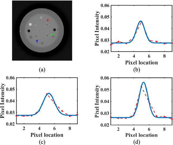
(a) High-dose CatPhan 600; Gaussian fitting of source points: (b) corresponding to the blue arrow, (c) corresponding to the red arrow, (d) corresponding to the green arrow. The blue curves indicate the fitting curve, and the red dotted curves represent the attenuation coefficients along the line segments centered at the source points.
TABLE I.
Blur Degree (FWHM) of Selected Locations in Catphan 600
| Source Point | High-dose | Low-dose |
|---|---|---|
| Green | 1.32 | 1.17 |
| Blue | 1.28 | 1.93 |
| Red | 1.74 | 1.67 |
|
| ||
| Mean | 1.45 | 1.59 |
We used the mean PSF of multiple source points in the high-dose FDK reconstruction results to approximate the blurring kernel. The reasons are as follows. First, the low-dose FDK reconstruction contains high noise levels, which might affect PSF estimation accuracy. Second, estimating a PSF map for the whole field of view would be hard and time-consuming. We assumed that the whole image has the same PSF for simplicity. Third, our experiments showed that the blurring kernel that was estimated using this method worked well. The kernel size was chosen to be 9×9.
D. Pure Reconstruction
The objective function of Eq. (6) can be written as:
| (8) |
and its derivative is expressed as:
| (9) |
The objective function Φ1 (x) is convex, and its minimizer can be obtained by ∂Φ1 (x)/∂x = 0, which can be solved using the Gauss-Seidel update strategy [51]. The initialization of the Gauss-Seidel iterative algorithms was set as the FDK reconstruction result, and the parameters in the Gauss-Seidel iterative algorithms were set as:
| (10) |
where and sj are intermediate variables and aj is the j th column of A. In the calculation of Σ reported above, we used the measured projection pi to approximate the mean projection since the mean projection was unknown in practice, as previously reported [19, 51]. For each j, the iterative process is expressed as:
| (11) |
In the reconstruction process, we adopted separable footprint (SF) projectors [53] to determine projection matrix A. We specifically used the SF projector with a trapezoid/rectangle function (SF-TR) [53]. SF-TR approximates the voxel footprint functions as 2D separable functions, and uses the trapezoid function in the transaxial direction and the rectangular function in the axial direction.
E. Deblurring based on CNN
The objection function of Eq. (7) can be re-written as:
| (12) |
with η = β/λ. This is a standard form of the deblurring problem. To fit the pure reconstruction sub-problem that generates reconstruction results with different blurring kernels and noise levels at different iterations, we used an iterative deblurring method [34] instead of other direct deblurring methods [37, 38].
Using again the half quadratic splitting method [49], Eq. (12) can be rewritten as:
| (13) |
Eq. (13)) can be solved through the following iterative process:
| (14) |
| (15) |
where Φ= η/ξ. Eq. (14) is a quadratic regularized least square problem, which can be solved using many methods. We selected a Fast Fourier Transform (FFT) method for this problem because of its computational efficiency. More details are reported in Appendix A. Eq. (15) corresponds to a denoising problem, which we solved by using a neural network method. To facilitate and reinforce the training phase, we combined the residual learning [34] and the image transfer net [46, 54]. The structure of our network is illustrated in Fig. 2.
Fig. 2.
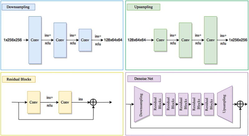
The architecture of our denoising network. Ins represents the instance normalization, conv represents the convolution operation, and relu represents the rectified linear units
The proposed network consists of one down-sampling, five residual blocks, and one up-sampling block. In the down-sampling and up-sampling blocks, we used the stride and fractional convolution instead of pooling layers, and used a reflection pad to keep the size. All non-residual convolutional layers were followed by instance normalization [54]. More details about the network are described in the following sections.
Dataset
Many datasets are available to train our network, including T91, BSDS200, General100 [39], and Imagenet [55]. We used the COCO dataset [56], which contains nearly 80 thousand images. We converted color images to gray images through the formula Gray = 0.299R + 0.587G + 0.114B.
Inputs and Outputs
Inputs included images from the COCO dataset, with the Gaussian noise of a certain level, and outputs included the corresponding Gaussian noise. Inputs and outputs were both randomly cropped gray images of 1×256×256.
Down-sampling and Up-sampling
The down-sampling process used a large stride to shrink the input image from 256 to 64. The up-sampling process used the nearest neighboring pixel value to enlarge the image from 64 to 256. A reflection pad was used to keep the size in the convolution phase.
Residual Blocks
The residual blocks can help train a very deep network and enable the network to learn how to identify the function [57].
Instance Normalization and Residual Learning
With the help of instance normalization, we trained our network in different batch sizes, which is important to fully use GPU memory and obtain a similar performance in different batch sizes. Residual learning helped us focus on noise rather than the image itself, reducing training convergence time and also helping to design a general denoiser.
Algorithm 1.
Loss Function
We used the simple least square form:
| (16) |
where F is the neural network operation, M is the batch size, xk, yk are the kth noise image, and the kth original image in the batch, respectively. This loss function corresponds to the peak signal to noise (PSNR), and is also recommended to define the loss function in the feature layers [44, 45].
Our network presents several advantages when compared to DnCNN [33, 34]. First, the number of weights in the middle process was reduced by using the down-sampling and up-sampling processes, allowing us to design a deeper and more powerful network. Second, using instance normalization instead of batch normalization, we can use a smaller batch size, lightening our burden to select the image size and dividing the image into many patches. Third, other pre-processes were not needed in the images, including image enhancement or flipping. By using the ADAM optimization method [58] without any tricks applied to the training phase, our network achieved the same performance level as that of DnCNN. Finally, our network converged quickly, and the training took only 4 hours on GTX1080Ti.
Iteration-based deblurring needs various denoisers with various noise levels, but considering all the cases is challenging and time-consuming. Using an inexact sub-problem solution can be a reasonable method [59]. In our network, every single denoiser in the deblurring process does not need to be fully functional in each iteration. The deblurring process gradually improved its performance during the iterative process. The iterative method can also potentially help us use the Gaussian denoiser to handle the deblurring problem with other noise types because different types of noise tend to be statistically similar at low noise levels. We trained 25 denoisers in the noise variation level [0, 50], as previously reported by Zhang et al. [34]. Our experiment results showed that this range of noise level worked well.
F. Parameter Selection
The parameters that need to be set up in our algorithm can be divided into two groups: (a) Parameter for pure reconstruction, λ; (b) Parameters for deblurring, ξ and η.
The objective function of the pure reconstruction sub-problem is Φ1 (x) (see Eq. (8)), and λ is a parameter that balances the reconstruction (p − Ax)T Σ−1 (p − Ax) and the deblurred part . Theoretically, if λ is too large, the result of the Gauss-Seidel iterative algorithm x will be enforced to approach Gu. If λ is too small, the reconstruction sub-problem and the deblurring sub-problem tend to become de-coupled. In our experiments, we empirically set λ in the near order of magnitude as sj. Specifically, parameter λ was set to 75000 for the CS phantom, and 30000 for the physical phantom and clinical patient data.
The objective function of the deblurring sub-problem is Φ2 (x) (see Eq. (12)), and this function can be divided between Eq. (14) and Eq. (15). The minimizer for the optimization problem in Eq. (15) corresponds to a Gaussian denoiser with noise level . In addition, the noise level of a reconstructed image would decrease gradually during the whole iteration process, indicating that a different denoiser trained over a different noise level should be used in each iteration. To lighten the burden of parameter selection, deblur-ring parameters ξ and η were set so that the ratio Φ = η/ξ would decrease linearly during reconstruction [34].
G. Algorithm
The pseudo code of our algorithm is reported as follows:
Note: n1 is the iteration number for the whole algorithm, n2 is the iteration number inside the deblurring process consisting of the least square problem (Eq. (14)) and the denoise problem (Eq. (15)). We used the Gauss-Seidel update strategy, FFT, and the denoising network to update x, u, and z respectively.
III. Materials and Evaluation
Two simulation phantoms (Compressed Sensing (CS) phantom, a modified Shepp-Logan Phantom), two physical phantoms (CatPhan 600, anthropomorphic head phantom), and data from a clinic patient were used to test our reconstruction algorithm.
A. Synthetic Phantom
The CS and the 3D Shepp-Logan phantoms were used for simulation. Their projection data covered 360 angles acquired by the SF algorithm [53]. Both phantoms contain 350×350×16 pixels, with an individual physical size of 0.776×0.776×0.776 mm3. Different Gaussian noise levels were simulated as different phantoms at different dose levels. The distance from source to detector is 150 cm and the distance from the object axis to detector is 50 cm for both simulated phantoms.
B. Physical Phantom
Projection data of the CatPhan 600 and anthropomorphic head, two physical phantoms, were acquired using a Varian Acuity system (Varian Medical System, Palo Alto, CA) with 125 kVp voltage. The X-ray tube current was set to 10 mA for low doses and 80mA for high doses. The projection image was of size 1024×768. The number of projections was 634 covering 360 degrees. Sizes were 350×350×16 for the CatPhan phantom and 550×550×32 for the head phantom. The physical size of each pixel was 0.776×0.776×0.776 mm3 and 0.388×0.388×0.388 mm3 for the CatPhan phantom and the head phantom, respectively. The distance between source and detector was 150 cm and the distance between axis and detector was 50 cm for both phantoms.
C. Patient Data
CBCT images were also acquired from a head and neck patient with a Varian Acuity system using a high-dose protocol of 80mA and 25ms, and a low-dose protocol of 20mA and 20ms. The X-ray tube was set to 100 kVp voltage. The reconstruction image was 500 ×500×16, the size of each pixel was 0.5×0.5×0.5 mm3, and the number of projections was 365 covering over 200 degrees.
D. Evaluation Criteria
PSNR, improvement signal to noise ratio (ISNR), structural similarity (SSIM), and contrast-to-noise ratio (CNR) were adopted to evaluate the reconstructed images. Since noise-free images were unavailable for the physical phantoms, we chose the FDK reconstruction images of high-dose level as reference. The quality of the reconstructed images depended on the selected parameters. To make the reconstructed images comparable across different methods, their noise levels were adjusted to be similar to one another. For the proposed algorithm, we fixed the pure reconstruction parameter λ and adjusted the noise level by using different deblurring parameters. Noise level was calculated as the average standard deviation of the selected regions. The definitions of PSNR, ISNR, SSIM, and CNR have been described [19].
IV. Experiments
A. CS Phantom
A representative slice of the noise-free image of the CS Phantom is shown in Fig. 3. Five blue rectangles were used to calculate noise levels. All the images reconstructed by different methods were adjusted to have the same noise level for fair comparison. The red rectangles were chosen as the region of interest (ROI) to reflect the quality of different methods.
Fig. 3.
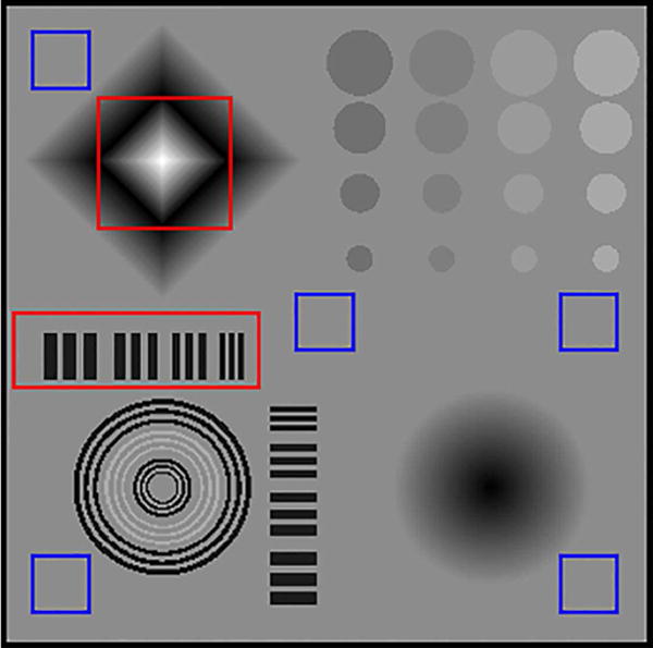
The original noise-free CS phantom
The enlarged rhombus ROI of the reconstruction results by FDK, TV, and our proposed method with incident photon number 5×10³ is shown in Fig. 4(a-c). The ROI results with incident photon number 1×10⁴ are shown in Fig. 4(d-f), and the ROI results with incident photon number 5 × 10⁴ are shown in Fig. 4(g-i). As observed in the reconstruction results, the FDK algorithm failed to reduce noise and caused significant artifacts. The TV penalty led to a serious staircase effect and several artificial piecewise constant regions. The images reconstructed using our method were more natural and smooth, indicating the ability of our method to preserve smooth regions in addition to suppressing noise.
Fig. 4.
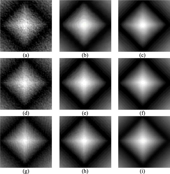
Zoom-in visual inspections of ROI (rhombus) of images reconstructed by different algorithms with different incident numbers. FDK: (a) high noise level; (d) medium noise level; (g) low noise level; TV: (b) high noise level; (e) medium noise level; (h) low noise level; Our method: (c) high noise level; (f) medium noise level; (i) low noise level
To evaluate our method in the edge area, the strip area (Barcode) was selected (Fig. 5). For all dose levels, visual inspection showed that both the TV penalty and the proposed method preserved the edges and suppressed the noise well. In contrast, the FDK method generated noise. A FWHM check along the red line in Fig. 5(c) indicated that our method had better spatial resolution (0.59 vs. 1.55) than the TV penalty, at low-dose levels.
Fig. 5.
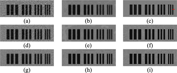
Zoom-in visual inspections of ROI (Barcode) of images reconstructed by different algorithms with different incident numbers. FDK: (a) high noise level; (d) medium noise level; (g) low noise level; TV: (b) high noise level; (e) medium noise level; (h) low noise level; Our method: (c) high noise level; (f) medium noise level; (i) low noise level
To quantify the reconstruction image with different methods, PSNR, ISNR, and SSIM of the whole slice and also the two selected ROIs were listed in Table II, III, and IV, respectively. The valuation indexes of our proposed method were found to be the highest at all dose levels.
TABLE II.
PSNR, ISNR, and SSIM Values of Images By Different Reconstruction Algorithms For The Cs Phantom
| Incident photon | Penalty | Noise level (×10−5) | PSNR | I SNR | SSIM |
|---|---|---|---|---|---|
| 5×10³ | FDK | 120 | 23.85 | / | 0.42 |
| TV | 3.51 | 29.82 | 5.97 | 0.96 | |
| Ours | 3.46 | 33.95 | 10.10 | 0.97 | |
| 1×10⁴ | FDK. | 95.20 | 25.66 | / | 0.54 |
| TV | 2.79 | 31.32 | 5.66 | 0.97 | |
| Ours | 2.74 | 35.18 | 9.52 | 0.99 | |
| 5×10⁴ | FDK | 52.10 | 27.93 | / | 0.77 |
| TV | 1.96 | 36.97 | 9.04 | 0.99 | |
| Ours | 1.96 | 38.27 | 10.34 | 0.99 |
TABLE III.
PSNR, ISNR, and SSIM Values of ROI (rhombus) by Different Reconstruction Algorithms for the Cs Phantom
| Incident photon | Penalty | Noise level (×10−5) | PSNR | I SNR | SSIM |
|---|---|---|---|---|---|
| 5×10³ | FDK | 120 | 25.76 | / | 0.66 |
| TV | 3.51 | 35.38 | 9.61 | 0.95 | |
| Ours | 3.46 | 38.32 | 12.55 | 0.98 | |
| 1×10⁴ | FDK | 95.20 | 28.84 | / | 0.79 |
| TV | 2.79 | 36.72 | 7.87 | 0.96 | |
| Ours | 2.74 | 39.36 | 10.52 | 0.98 | |
| 5×10⁴ | FDK | 52.10 | 33.93 | / | 0.93 |
| TV | 1.96 | 39.98 | 6.05 | 0.98 | |
| Ours | 1.96 | 40.87 | 6.94 | 0.98 |
TABLE IV.
PSNR, ISNR, and SSIM Values of ROI (Barcode) by Different Reconstruction Algorithms for the Cs Phantom
| Incident photon | Penalty | Noise level (×10−5) | PSNR | ISNR | SSIM |
|---|---|---|---|---|---|
| 5×10³ | FDK | 120 | 17.61 | / | 0.76 |
| TV | 3.51 | 21.91 | 5.97 | 0.96 | |
| Ours | 3.46 | 28.89 | 11.29 | 0.99 | |
| 1×10⁴ | FDK | 95.20 | 19.22 | / | 0.82 |
| TV | 2.79 | 24.39 | 5.17 | 0.97 | |
| Ours | 2.74 | 30.78 | 11.56 | 0.99 | |
| 5×10⁴ | FDK | 52.10 | 20.82 | / | 0.90 |
| TV | 1.96 | 32.65 | 11.83 | 1.00 | |
| Ours | 1.96 | 33.26 | 12.43 | 1.00 |
B. Modified 3D Shepp-Logan Phantom
The 3D Shepp-Logan phantom was modified by replacing the constant ellipsoid with one containing linearly changed intensity. A representative slice of the modified 3D Shepp-Logan phantom obtained by different methods is displayed in Fig. 6. The original image is illustrated in Fig. 6(a), and the image reconstructed by different methods is illustrated in Fig. 6(b-d). The white rectangles were selected as background to calculate noise levels. The yellow rectangle indicates the ROI, which is displayed in the lower right corner in Fig. 6(a–d). Our proposed method can successfully avoid the staircase effect and preserve the smooth region. In contrast, the FDK reconstruction image contains too much noise, and the TV penalty shows an obvious staircase effect.
Fig. 6.
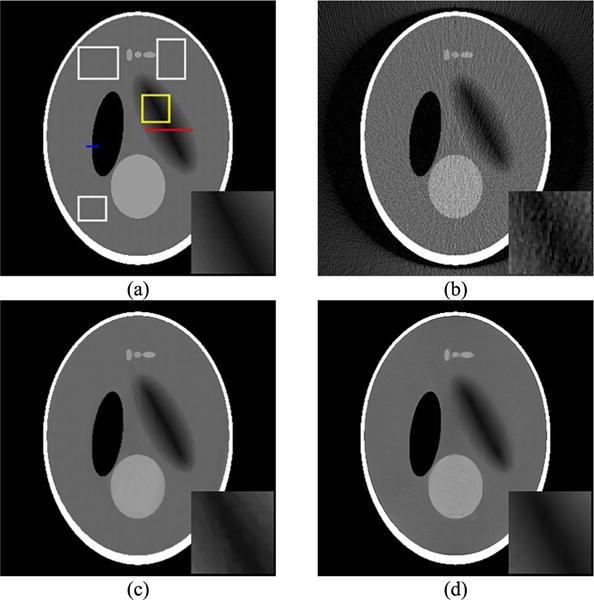
A representative slice of the 3D Shepp-Logan Phantom reconstructed by different methods: (a) Original image; (b) FDK; (c) TV; (d) Ours
The change of image intensity along the red line in Fig. 6(a) is illustrated in Fig. 7. These plots indicate that the TV penalty produces piecewise constant artifacts, while the proposed method exhibits better reconstruction quality.
Fig. 7.
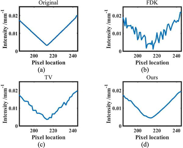
Profiles through the ellipsoid object (the red line in Fig. 6(a)): (a) Original image; (b) FDK; (c) TV; (d) Ours
As for image resolution, we selected the blue line in Fig. 6(a) to calculate the FWHM. The FWHM value of the TV penalty was 1.8597, and that of our method was 0.5821, indicating a higher image resolution for our method.
C. CatPhan 600 Phantom
A representative slice of the reconstructed CatPhan600 phantom images generated with different methods are shown in Fig. 8. The blue rectangle area was used to calculate noise level. Since we cannot obtain noise-free images, we selected three ROIs, to measure and quantitatively compare CNR between different reconstruction methods (indicated by the arrows in Fig. 8(a)).
Fig. 8.
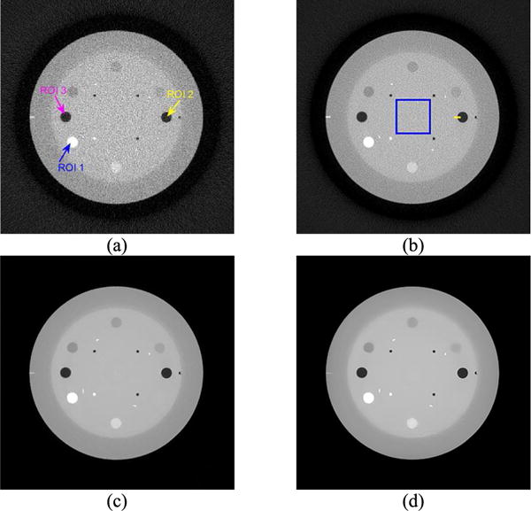
Representative slices from the reconstructed CatPhan 600 images. (a) FDK with high-dose protocol (80mA/10ms); (b) FDK with Low-dose protocol (10mA/10ms); (c) TV (low-dose); (d) Ours (low-dose)
The evaluation indexes are listed in Table V. Our method performed better than the TV penalty in denoising.
TABLE V.
CNRs oF Different ROIs of the Catphan 600 Phantom
| Noise(×10−4) | ROI1 | ROI2 | ROB | |
|---|---|---|---|---|
| FDK_10mA | 24 | 3.55 | 5.37 | 5.22 |
| FDK_80mA | 9.15 | 9.64 | 12.76 | 12.63 |
| TV | 1.16 | 70.40 | 87.49 | 74.95 |
| Ours | 1.15 | 82.58 | 113.41 | 94.47 |
Since CNR depends highly on the background noise level, its values present limitations in evaluating the quality of the reconstructed images. To emphasize the importance of our method in deblurring, we drew a yellow line to calculate FWHM (Fig. 8(b)). The FWHM of the TV penalty is 1.9477 and that of our method is 1.7932, indicating higher image resolution for our method. To check if the proposed algorithm is universal and adaptive, we calculated FWHM values for images reconstructed with different noise levels (Fig. 9). The image resolution of our method changed only slightly (FWHM values decreased by 0.4% from 1.8143 to 1.8068) when the noise level was increased by 140% from 4×10⁻⁵ to 12 ×10−5 (Fig. 9). Table V and Fig. 9 indicated that our method can efficiently suppress both noise and blurring effect, providing high image resolution (Table V and Fig. 9).
Fig. 9.
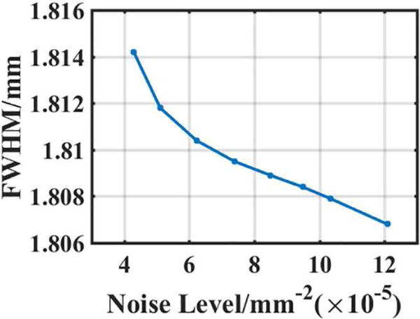
FWHM Values-Noise Level curves
D. Anthropomorphic Head Phantom
A representative slice of the results obtained using different reconstruction methods for the head phantom are illustrated in Fig. 10. The red rectangle area was selected as the ROI, and the white rectangle area was used to measure noise levels (Fig. 10(b)). The reconstructions of the proposed algorithm and TV were within the same noise level. The high dose FDK reconstruction image was chosen as reference because the original noise-free image was unavailable. We used the SSIM to evaluate the similarity degree of the local structures between the reconstruction images and the high dose FDK image. Our method had a whiter SSIM map of the anthropomorphic head phantom (Fig 11), indicating a better ability to preserve structures. The mean SSIM (MSSIM) value in the selected ROI is listed in Table VI, revealing that our method had the best structure-preserving ability.
Fig. 10.
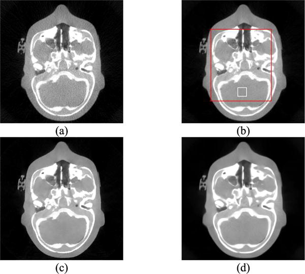
A representative slices of the reconstructed anthropomorphic head phantom image using different penalties: (a) FDK low-dose protocol (10mA/10ms); (b) FDK high-dose protocol (80mA/10ms); (c) TV (low-dose); (d) Ours (low-dose)
Fig. 11.
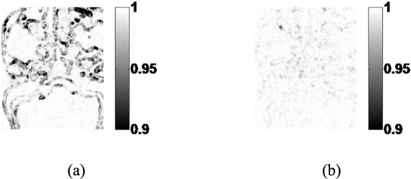
SSIM map of the head phantom using different methods. (a). TV (SSIM=0.9861), (b). Ours (SSIM=0.9964)
TABLE VI.
MSSIM of the Red ROI shown in Fig. 10 (B)
| Penalty | Noise level(×10−4) | SSIM |
|---|---|---|
| FDK_10mA | 17 | 0.74 |
| FDK_80mA | 8.54 | N/A |
| TV | 4.88 | 0.97 |
| Ours | 4.87 | 1.00 |
E. Patient results
The results of the FDK reconstruction on patient data acquired with different dose levels are shown in Fig. 12 (a-b). The low dose results using the TV penalty and the proposed method are shown in Fig. 12 (c-d). The white rectangle on the background was selected to measure noise levels. The noise levels for the FDK low-dose protocol, FDK high-dose protocol, SIR with the TV penalty and our algorithm were found to be 29 ×10−4, 14×10−4, 6.52×10⁻⁴, and 6.75 ×10⁻⁴, respectively. The red line in the image was selected to calculate the FWHM value and test the deblurring effect. The FWHM of our method is 1.7145, while that of the TV penalty is 3.0090 with. These results suggest that our method had higher spatial resolution than TV. The red rectangle is displayed in the lower right corner to illustrate the performance of different reconstruction methods. Visual results obtained by our proposed method were more similar to those of the reference high dose FDK reconstruction, than to those of the traditional TV penalty.
Fig. 12.
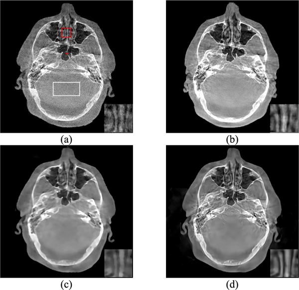
A representative slice of the reconstructed patient data using different penalties: (a) FDK low-dose protocol (20mA/20ms, nose level: 29×10−4); (b) FDK high-dose protocol (80mA/25ms, nose level: 14×10−4); (c) TV (nose level: 6.52×10⁻⁴) and (d) Ours (nose level: 6.75×10⁻⁴), both using the low-dose protocol
V. Discussion
In statistical iterative reconstruction, the regularization term represents prior information on the target image, and plays an important role for reconstruction quality. Many regularization terms such as TV and Hessian have been proposed because of their good performance. However, because the manually designed regularization term is based primarily on the researchers’ knowledge about the problem, effective regularization is often hard to design. We proposed using the network to learn the “potential regularization term” through data. This shifts the problem of designing the regularization term to the problem of training the neural network.
The major challenge of applying CNN to SIR is where and what role it should play in the iteration process. Considering that the amount of normal-dose CBCT images is low and that these images are no way to be noiseless in practice, we used transfer learning [33] to train the network on natural images. Instead of training a network end-to-end [43], we arranged for the neural network to play the role of a regularization term, which can be embedded into different inverse problems. To adapt to the SIR process, which might have different blurring kernels and noise levels in every iterative phase, we used an iterative deblurring method consisting of a CNN denoiser and a quadratic regularized least-square problem. The iterative deblurring method possibly can also deal with different kinds of noise that benefit CBCT reconstruction problems in which the noise type may be unknown. One of the major advantages of the proposed reconstruction method is integrating CNN into the iterative reconstruction, adding extra flexibility and extendibility compared to other CNN-based CBCT reconstruction methods [43, 44].
Eq. (15) corresponds to a Gaussian denoising problem, and the regularization term in Eq. (15) plays a role in enforcing the solution to be more similar to a noise-free CBCT image. Traditionally, the key is to design a proper regularization term R (u) for the denoising problem. We used a neural network to solve the denoising problem. The corresponding form of a neural network solution can be represented as z = F (u) (Please see Eq. (15)). The neural network method solves the denoising problem by learning F. The learnt denoiser-using network can be viewed as learning a “potential regularization term” through data. Dmitry Ulyanov et al. found that the network is sufficient to capture rich low-level image statistics [60]. The regularization term in Eq. (15) was exactly the same as that in Eq. (4). Thanks to the variable splitting technique, the optimization of Eq. (15) (or denoising) using the neural network is equivalent to learning the regularization term for the entire algorithm (Eq. (4)) via the neural network.
Our findings indicate that our network-based SIR can successfully eliminate the staircase effect and preserve both edges and image regions with smooth intensity transition. The traditional SIR with a specially designed penalty term often needs to adjust the parameters to balance noise levels and image resolution, which is typically time-consuming. In contrast, our method can potentially provide reconstruction images with low noise level, while maintaining high image resolution.
Although our network-based SIR showed good performance, several aspects need to be improved. First, the deblurring process might not be thorough due to the rough PSF estimation (using a linear decreasing way), which may reduce image resolution. This limitation may be addressed by designing a dynamic PSF estimation process. Second, as shown in the CS experiment, different regions of the images exhibited different noise levels. Also, the network did not work well for local regions where the background was close to the foreground, indicating the need to design a more “intelligent” network. Third, we trained the network using 25 different noise levels, which are not elegant enough, indicating the need to design a more common denoiser. Finally, as shown in our CatPhan600 experiments, the small bright structure on the left of the phantom (Fig. 8 (a)) became dim when our algorithm was used (Fig. 8 (d)). Interestingly, reconstruction using the TV penalty underwent a similar phenomenon (Fig. 8(c)). In our algorithm, parameter λ in Eq. (6) still played a similar role to the regularization parameter in a standard inverse problem formulation. In this formulation, a large regularization parameter will generally make the solution smoother. The objective function in Eq. (6) used a quadratic “penalty” that was introduced by the variable splitting technique. A quadratic penalty is known to over-smooth the solution in a standard inverse problem. In this sense, the quadratic “penalty” might be an inherent shortcoming of the proposed algorithm. One way to improve the current version of our proposed algorithm is to use other variable splitting techniques that lead to other “penalties” (e.g. non-quadratic) that better preserve small and faint structures.
VI. Conclusion
We proposed a new network-based iterative CBCT reconstruction method that addresses issues such as data deficiency and unknown noise level to train the network. Our proposed SIR method solves the CBCT reconstruction problem innovatively. The data-driven approach that learns the “potential regularization term” overcomes the challenge of designing penalty terms in traditional SIR methods. Our studies conducted in simulated and physical phantoms, and also on data from a clinic patient showed that our method can eliminate the staircase effect and preserve both edges and regions with smooth intensity transition.
Acknowledgments
We would like to thank Dr. Damiana Chiavolini for editing the paper.
This work was supported in part by the National Natural Science Foundation of China (NNSFC), under Grant Nos. 61375018 and 61672253. J. Wang was supported in part by grants from the Cancer Prevention and Research Institute of Texas (RP160661) and the National Institute of Biomedical Imaging and Bioengineering (R01 EB020366).
Appendix
A. Solve Quadratic Regularized Least Squares
We defined several symbols as follows: ⊗: convolution, ○: dot product, k: frequency domain coordinates, : conjugate transpose.
Rewrite Eq. (14) as follow:
| (A-1) |
Introduce a new matrix M: the same size as G and every element in M is 0 excluding the center element which is 1. Eq. (A-1) now became:
| (A-2) |
Letting ∂Φ1/∂u = 0 and applying Fourier transform, we obtained
| (A-3) |
Using IFFT, we can obtain the solution of u.
Contributor Information
Binbin Chen, School of Automation, Huazhong University of Science and Technology, Wuhan, China.
Kai Xiang, School of Automation, Huazhong University of Science and Technology, Wuhan, China.
Zaiwen Gong, School of Automation, Huazhong University of Science and Technology, Wuhan, China.
Jing Wang, Department of Radiation Oncology, University of Texas Southwestern Medical Center, Texas, USA.
Shan Tan, School of Automation, Huazhong University of Science and Technology, Wuhan, China.
References
- 1.de González AB, Mahesh M, Kim K-P, Bhargavan M, Lewis R, Mettler F, et al. Projected cancer risks from computed tomographic scans performed in the United States in 2007. Archives of internal medicine. 2009;169:2071–2077. doi: 10.1001/archinternmed.2009.440. [DOI] [PMC free article] [PubMed] [Google Scholar]
- 2.Wen N, Guan H, Hammoud R, Pradhan D, Nurushev T, Li S, et al. Dose delivered from Varian’s CBCT to patients receiving IMRT for prostate cancer. Physics in medicine and biology. 2007;52:2267. doi: 10.1088/0031-9155/52/8/015. [DOI] [PubMed] [Google Scholar]
- 3.Hsieh J. Adaptive streak artifact reduction in computed tomography resulting from excessive x -ray photon noise. Medical Physics. 1998;25:2139–2147. doi: 10.1118/1.598410. [DOI] [PubMed] [Google Scholar]
- 4.Kachelrieß M, Watzke O, Kalender WA. Generalized multi-dimensional adaptive filtering for conventional and spiral single - slice, multi - slice, and cone - beam CT. Medical Physics. 2001;28:475–490. doi: 10.1118/1.1358303. [DOI] [PubMed] [Google Scholar]
- 5.Wang J, Lu H, Liang Z, Eremina D, Zhang G, Wang S, et al. An experimental study on the noise properties of x-ray CT sinogram data in Radon space. Physics in medicine and biology. 2008;53:3327. doi: 10.1088/0031-9155/53/12/018. [DOI] [PMC free article] [PubMed] [Google Scholar]
- 6.Huang H-M, Hsiao T. Accelerating an ordered-subset low-dose X-ray cone beam computed tomography image reconstruction with a power factor and total variation minimization. PloS one. 2016;11:e0153421. doi: 10.1371/journal.pone.0153421. [DOI] [PMC free article] [PubMed] [Google Scholar]
- 7.Jia X, Lou Y, Lewis J, Li R, Gu X, Men C, et al. GPU-based fast low-dose cone beam CT reconstruction via total variation. Journal of X-ray science and technology. 2011;19:139–154. doi: 10.3233/XST-2011-0283. [DOI] [PubMed] [Google Scholar]
- 8.Rudin LI, Osher S, Fatemi E. Nonlinear total variation based noise removal algorithms. Physica D: Nonlinear Phenomena. 1992;60:259–268. [Google Scholar]
- 9.Sidky EY, Pan X. Image reconstruction in circular cone-beam computed tomography by constrained, total-variation minimization. Physics in medicine and biology. 2008;53:4777. doi: 10.1088/0031-9155/53/17/021. [DOI] [PMC free article] [PubMed] [Google Scholar]
- 10.Zhang Y, Tehrani JN, Wang J. A biomechanical modeling guided CBCT estimation technique. IEEE transactions on medical imaging. 2017;36:641–652. doi: 10.1109/TMI.2016.2623745. [DOI] [PMC free article] [PubMed] [Google Scholar]
- 11.Jia X, Lou Y, Li R, Song WY, Jiang SB. GPU - based fast cone beam CT reconstruction from undersampled and noisy projection data via total variation. Medical physics. 2010;37:1757–1760. doi: 10.1118/1.3371691. [DOI] [PubMed] [Google Scholar]
- 12.Sidky EY, Kao C-M, Pan X. Accurate image reconstruction from few-views and limited-angle data in divergent-beam CT. Journal of X-ray Science and Technology. 2006;14:119–139. [Google Scholar]
- 13.Bredies K, Kunisch K, Pock T. Total generalized variation. SIAM Journal on Imaging Sciences. 2010;3:492–526. [Google Scholar]
- 14.You Y-L, Kaveh M. Fourth-order partial differential equations for noise removal. IEEE Transactions on Image Processing. 2000;9:1723–1730. doi: 10.1109/83.869184. [DOI] [PubMed] [Google Scholar]
- 15.Hu Y, Jacob M. Higher degree total variation (HDTV) regularization for image recovery. IEEE Transactions on Image Processing. 2012;21:2559–2571. doi: 10.1109/TIP.2012.2183143. [DOI] [PubMed] [Google Scholar]
- 16.Lefkimmiatis S, Ward JP, Unser M. Hessian Schatten-norm regularization for linear inverse problems. IEEE transactions on image processing. 2013;22:1873–1888. doi: 10.1109/TIP.2013.2237919. [DOI] [PubMed] [Google Scholar]
- 17.Liu J, Huang T-Z, Selesnick IW, Lv X-G, Chen P-Y. Image restoration using total variation with overlapping group sparsity. Information Sciences. 2015;295:232–246. [Google Scholar]
- 18.Shi Q, Sun N, Sun T, Wang J, Tan S. Structure-adaptive CBCT reconstruction using weighted total variation and Hessian penalties. Biomed Opt Express. 2016 Sep 01;7:3299–3322. doi: 10.1364/BOE.7.003299. [DOI] [PMC free article] [PubMed] [Google Scholar]
- 19.Sun T, Sun N, Wang J, Tan S. Iterative CBCT reconstruction using Hessian penalty. Physics in medicine and biology. 2015;60:1965. doi: 10.1088/0031-9155/60/5/1965. [DOI] [PubMed] [Google Scholar]
- 20.Jia X, Dong B, Lou Y, Jiang SB. GPU-based iterative cone-beam CT reconstruction using tight frame regularization. Physics in medicine and biology. 2011;56:3787. doi: 10.1088/0031-9155/56/13/004. [DOI] [PubMed] [Google Scholar]
- 21.Xu Q, Yu H, Mou X, Zhang L, Hsieh J, Wang G. Low-Dose X-ray CT Reconstruction via Dictionary Learning. IEEE transactions on medical imaging. 2012 Apr 20;31:1682–1697. doi: 10.1109/TMI.2012.2195669. [DOI] [PMC free article] [PubMed] [Google Scholar]
- 22.Lu Y, Zhao J, Wang G. Few-view image reconstruction with dual dictionaries. Physics in medicine and biology. 2011;57:173. doi: 10.1088/0031-9155/57/1/173. [DOI] [PMC free article] [PubMed] [Google Scholar]
- 23.Choi K, Wang J, Zhu L, Suh TS, Boyd S, Xing L. Compressed sensing based cone - beam computed tomography reconstruction with a first - order method. Medical physics. 2010;37:5113–5125. doi: 10.1118/1.3481510. [DOI] [PMC free article] [PubMed] [Google Scholar]
- 24.Ravishankar S, Moore BE, Nadakuditi RR, Fessler JA. Low-Rank and Adaptive Sparse Signal (LASSI) Models for Highly Accelerated Dynamic Imaging. IEEE Transactions on Medical Imaging. 2017;36:1116–1128. doi: 10.1109/TMI.2017.2650960. [DOI] [PMC free article] [PubMed] [Google Scholar]
- 25.Kim K, Ye JC, Worstell W, Ouyang J, Rakvongthai Y, Fakhri GE, et al. Sparse-View Spectral CT Reconstruction Using Spectral Patch-Based Low-Rank Penalty. IEEE Transactions on Medical Imaging. 2015;34:748–760. doi: 10.1109/TMI.2014.2380993. [DOI] [PubMed] [Google Scholar]
- 26.Zhang H, Huang J, Ma J, Bian Z, Feng Q, Lu H, et al. Iterative reconstruction for X-ray computed tomography using prior-image induced nonlocal regularization. IEEE Transactions on Biomedical Engineering. 2014;61:2367–2378. doi: 10.1109/TBME.2013.2287244. [DOI] [PMC free article] [PubMed] [Google Scholar]
- 27.Niu S, Yu G, Ma J, Wang J. Nonlocal low-rank and sparse matrix decomposition for spectral CT reconstruction. Inverse Problems. 2017 doi: 10.1088/1361-6420/aa942c. [DOI] [PMC free article] [PubMed] [Google Scholar]
- 28.Hao J, Zhang L, Li L, Kang K. An improved non-local means regularized iterative reconstruction method for low-dose dental CBCT. Nuclear Science Symposium and Medical Imaging Conference (NSS/MIC), 2012 IEEE. 2012:3422–3425. [Google Scholar]
- 29.Chen Y, Gao D, Nie C, Luo L, Chen W, Yin X, et al. Bayesian statistical reconstruction for low-dose X-ray computed tomography using an adaptive-weighting nonlocal prior. Computerized Medical Imaging and Graphics. 2009;33:495–500. doi: 10.1016/j.compmedimag.2008.12.007. [DOI] [PubMed] [Google Scholar]
- 30.Feruglio PF, Vinegoni C, Gros J, Sbarbati A, Weissleder R. Block matching 3D random noise filtering for absorption optical projection tomography. Physics in medicine and biology. 2010;55:5401. doi: 10.1088/0031-9155/55/18/009. [DOI] [PMC free article] [PubMed] [Google Scholar]
- 31.Choi Y, Koo J-Y, Lee N-Y. Image reconstruction using the wavelet transform for positron emission tomography. IEEE transactions on medical imaging. 2001;20:1188–1193. doi: 10.1109/42.963822. [DOI] [PubMed] [Google Scholar]
- 32.Cai J, Jia X, Gao H, Jiang S, Shen Z, Zhao H. Cine Cone Beam CT Reconstruction Using Low-Rank Matrix Factorization: Algorithm and a Proof-of-Principle Study. IEEE Transactions on Medical Imaging. 2014;33:1581–1591. doi: 10.1109/TMI.2014.2319055. [DOI] [PMC free article] [PubMed] [Google Scholar]
- 33.Zhang K, Zuo W, Chen Y, Meng D, Zhang L. Beyond a gaussian denoiser: Residual learning of deep cnn for image denoising. IEEE Transactions on Image Processing. 2017 doi: 10.1109/TIP.2017.2662206. [DOI] [PubMed] [Google Scholar]
- 34.Zhang K, Zuo W, Gu S, Zhang L. Learning Deep CNN Denoiser Prior for Image Restoration. arXiv preprint arXiv:1704.03264. 2017 [Google Scholar]
- 35.Zhang J, Pan J, Lai W-S, Lau R, Yang M-H. Learning Fully Convolutional Networks for Iterative Non-blind Deconvolution. arXiv preprint arXiv:1611.06495. 2016 [Google Scholar]
- 36.Lefkimmiatis S. Non-local color image denoising with convolutional neural networks. arXiv preprint arXiv:1611.06757. 2016 [Google Scholar]
- 37.Chakrabarti A. A neural approach to blind motion deblurring. European Conference on Computer Vision. 2016:221–235. [Google Scholar]
- 38.Wieschollek P, Schölkopf B, Lensch HP, Hirsch M. End-to-end learning for image burst deblurring. Asian Conference on Computer Vision. 2016:35–51. [Google Scholar]
- 39.Lai W-S, Huang J-B, Ahuja N, Yang M-H. Deep Laplacian Pyramid Networks for Fast and Accurate Super-Resolution. arXiv preprint arXiv:1704.03915. 2017 doi: 10.1109/TPAMI.2018.2865304. [DOI] [PubMed] [Google Scholar]
- 40.Ledig C, Theis L, Huszár F, Caballero J, Cunningham A, Acosta A, et al. Photo-realistic single image super-resolution using a generative adversarial network. arXiv preprint arXiv:1609.04802. 2016 [Google Scholar]
- 41.Wang G. A perspective on deep imaging. IEEE Access. 2016;4:8914–8924. [Google Scholar]
- 42.Kang E, Min J, Ye JC. A deep convolutional neural network using directional wavelets for low-dose X-ray CT reconstruction. arXiv preprint arXiv:1610.09736. 2016 doi: 10.1002/mp.12344. [DOI] [PubMed] [Google Scholar]
- 43.Chen H, Zhang Y, Zhang W, Liao P, Li K, Zhou J, et al. Low-dose CT via convolutional neural network. Biomedical optics express. 2017;8:679–694. doi: 10.1364/BOE.8.000679. [DOI] [PMC free article] [PubMed] [Google Scholar]
- 44.Yang Q, Yan P, Kalra MK, Wang G. CT Image Denoising with Perceptive Deep Neural Networks. arXiv preprint arXiv:1702.07019. 2017 [Google Scholar]
- 45.Gatys LA, Ecker AS, Bethge M. A neural algorithm of artistic style. arXiv preprint arXiv:1508.06576. 2015 [Google Scholar]
- 46.Johnson J, Alahi A, Fei-Fei L. Perceptual losses for real-time style transfer and super-resolution. European Conference on Computer Vision. 2016:694–711. [Google Scholar]
- 47.Arjovsky M, Chintala S, Bottou L. Wasserstein gan. arXiv preprint arXiv:1701.07875. 2017 [Google Scholar]
- 48.Yang Q, Yan P, Zhang Y, Yu H, Shi Y, Mou X, et al. Low Dose CT Image Denoising Using a Generative Adversarial Network with Wasser-stein Distance and Perceptual Loss. arXiv preprint arXiv:1708.00961. 2017 doi: 10.1109/TMI.2018.2827462. [DOI] [PMC free article] [PubMed] [Google Scholar]
- 49.Geman D, Yang C. Nonlinear image recovery with half-quadratic regularization. IEEE Transactions on Image Processing. 1995;4:932–946. doi: 10.1109/83.392335. [DOI] [PubMed] [Google Scholar]
- 50.Li T, Li X, Wang J, Wen J, Lu H, Hsieh J, et al. Nonlinear sinogram smoothing for low-dose X-ray CT. IEEE Transactions on Nuclear Science. 2004;51:2505–2513. [Google Scholar]
- 51.Wang J, Li T, Xing L. Iterative image reconstruction for CBCT using edge - preserving prior. Medical physics. 2009;36:252–260. doi: 10.1118/1.3036112. [DOI] [PMC free article] [PubMed] [Google Scholar]
- 52.Hashemi S, Song WY, Sahgal A, Lee Y, Huynh C, Grouza V, et al. Simultaneous deblurring and iterative reconstruction of CBCT for image guided brain radiosurgery. Physics in Medicine and Biology. 2017;62:2521. doi: 10.1088/1361-6560/aa5ed2. [DOI] [PubMed] [Google Scholar]
- 53.Long Y, Fessler JA, Balter JM. 3D forward and back-projection for X-ray CT using separable footprints. IEEE transactions on medical imaging. 2010;29:1839–1850. doi: 10.1109/TMI.2010.2050898. [DOI] [PMC free article] [PubMed] [Google Scholar]
- 54.Ulyanov D, Vedaldi A, Lempitsky V. Instance normalization: The missing ingredient for fast stylization. arXiv preprint arXiv:1607.08022. 2016 [Google Scholar]
- 55.Russakovsky O, Deng J, Su H, Krause J, Satheesh S, Ma S, et al. Imagenet large scale visual recognition challenge. International Journal of Computer Vision. 2015;115:211–252. [Google Scholar]
- 56.Lin T-Y, Maire M, Belongie S, Hays J, Perona P, Ramanan D, et al. Microsoft coco: Common objects in context. European conference on computer vision. 2014:740–755. [Google Scholar]
- 57.He K, Zhang X, Ren S, Sun J. Deep residual learning for image recognition. Proceedings of the IEEE conference on computer vision and pattern recognition. 2016:770–778. [Google Scholar]
- 58.Kingma D, Ba J. Adam: A method for stochastic optimization. arXiv preprint arXiv:1412.6980. 2014 [Google Scholar]
- 59.Lin Z, Chen M, Ma Y. The augmented lagrange multiplier method for exact recovery of corrupted low-rank matrices. arXiv preprint arXiv:1009.5055. 2010 [Google Scholar]
- 60.Ulyanov D, Vedaldi A, Lempitsky V. Deep Image Prior. arXiv preprint arXiv:1711.10925. 2017 [Google Scholar]