Two Representations of a High-Dimensional Perceptual Space

Abstract

A perceptual space is a mental workspace of points in a sensory domain that supports similarity and difference judgments and enables further processing such as classification and naming. Perceptual spaces are present across sensory modalities; examples include colors, faces, auditory textures, and odors. Color is perhaps the best-studied perceptual space, but it is atypical in two respects. First, the dimensions of color space are directly linked to the three cone absorption spectra, but the dimensions of generic perceptual spaces are not as readily traceable to single-neuron properties. Second, generic perceptual spaces have more than three dimensions. This is important because representing each distinguishable point in a high-dimensional space by a separate neuron or population is unwieldy; combinatorial strategies may be needed to overcome this hurdle.

To study the representation of a complex perceptual space, we focused on a well-characterized 10-dimensional domain of visual textures. Within this domain, we determine perceptual distances in a threshold task (segmentation) and a suprathreshold task (border salience comparison). In N=4 human observers, we find both quantitative and qualitative differences between these sets of measurements. Quantitatively, observers’ segmentation thresholds were inconsistent with their uncertainty determined from border salience comparisons. Qualitatively, segmentation thresholds suggested that distances are determined by a coordinate representation with Euclidean geometry. Border salience comparisons, in contrast, indicated a global curvature of the space, and that distances are determined by activity patterns across broadly tuned elements. Thus, our results indicate two representations of this perceptual space, and suggest that they use differing combinatorial strategies.

Introduction

Perceptual spaces are internal workspaces within a sensory modality. By providing a representation that captures similarities and differences, perceptual spaces form a stage of sensory processing that not only supports simple discrimination judgments but also enables higher levels of processing, such as classification and naming. Our goal here is to understand the nature of this representation, using the perceptual space of image statistics (Victor, Rizvi, & Conte, 2015) as a model. Along with (Edelman, 1998), our use of the term “representation” refers not only to the points of the perceptual space (i.e, to individual stimuli), but also, to similarity judgments (i.e., to how distances between stimuli are computed).

Among perceptual spaces, the space of human trichromatic color vision is the oldest and best known example (Maxwell, 1860). However, many other perceptual spaces have been identified: not only in vision (for faces (Catz, Kampf, Nachson, & Babkoff, 2009; Freiwald, Tsao, & Livingstone, 2009; Tanaka, Meixner, & Kantner, 2011; Valentine, 1991; Wallraven, 2014) and other objects (Wallraven, 2014)) but also in other sensory modalities (Bushdid, Magnasco, Vosshall, & Keller, 2014; Gaissert, Wallraven, & Bulthoff, 2010; Geffen, Gervain, Werker, & Magnasco, 2011; Koulakov, Kolterman, Enikolopov, & Rinberg, 2011; McDermott, Schemitsch, & Simoncelli, 2013; McDermott & Simoncelli, 2011; Yoshioka, Bensmaia, Craig, & Hsiao, 2007; Zaidi et al., 2013).

While color space is perhaps the most widely studied, many of its characteristics are not generic. For primate color vision, the properties of the three cone classes determine the dimensions of the space (Baylor, Nunn, & Schnapf, 1987), provide it with a coordinate system, and enable construction of stimuli that modulate each coordinate independently (Derrington, Krauskopf, & Lennie, 1984). For other perceptual spaces, the dimensionality is much larger, and these perceptual dimensions do not map in a straightforward way to the physics of the stimulus (Bushdid et al., 2014; Freiwald et al., 2009; Koulakov et al., 2011; Victor et al., 2015(Cho, Yang, & Hallett, 2000; Portilla & Simoncelli, 2000)). Thus, it is not even guaranteed that generic perceptual spaces have a coordinate system, or that it is possible to find a set of independent perceptual dimensions. Nevertheless, these more complex perceptual spaces also support threshold and suprathreshold judgments.

Because typical perceptual spaces are multi-dimensional, representing them via “brute-force” strategies – in which each discriminable stimulus is represented by a separate neuron (or neural population) – is biologically implausible, because of a dimensional explosion of the resources required. If there are D independent dimensions and N discriminable values on each of the corresponding axes, there would be N^D distinct points in the space. In the case of color (D = 3 and N >100), this leads to an estimate of over 10⁶ distinct stimuli (colors) that need to be represented. For olfactory stimuli, it is estimated that D is much larger than 10, (Koulakov et al., 2011), and the total number of discriminable stimuli has been estimated at >10¹² (Bushdid et al., 2014). The space of visual textures, the present focus, is also high-dimensional; to analyze how it is represented, we study regions within a well-characterized 10-dimensional subset (Victor & Conte, 2012; Victor et al., 2015).

The dimensional explosion in resources required for a brute-force representation can be mitigated by combinatorial strategies. One class of such strategies makes use of coordinates for the space (e.g., the amount of each color primary). By projecting the entire space onto each axis, a high-dimensional space can be efficiently represented in terms of its one-dimensional projections. A second class of strategies does not rely on a coordinate system in the usual sense, but instead postulates that neurons have a diverse set of broadly-tuned sensitivities. Interestingly, theoretical arguments suggest that this strategy becomes efficient for spaces of dimensionality D ≥ 3 (Zhang & Sejnowski, 1999).

While both kinds of strategies are combinatorial, they make contrasting predictions about distances. Consider an experiment that measures perceptual distance between test points that are displaced in opposite directions from a reference point near the center of the space. In this experiment, we measure the perceptual distance as the amount of the displacement increases – that is, as the test points are pulled further and further apart. In a coordinate-based representation, the perceptual distance can only increase – since the distance between the projections of the two test points onto any axis must increase, as the test points move away from the reference. But in a representation based on patterns of activity across broadly-tuned neurons, other outcomes are possible. For example, suppose that most of the neurons are tuned to regions near the center of the space, and very few of them cover its periphery – as would be expected from an efficient deployment of resources (Hermundstad et al., 2014). Then, as the test points move into the periphery, fewer and fewer neurons contribute to their representations, and they therefore become less distinguishable.

These considerations motivate our approach to probing the representation of visual textures. In one experiment, we measure discrimination thresholds; in another, we measure suprathreshold perceptual distances. Our results suggest that both kinds of combinatorial strategies are used to compute distances – a coordinate-based representation that accounts for discrimination thresholds, and a distributed representation that accounts for the global perceptual geometry of the space.

Materials and Methods

The experiments described here consist of two kinds of psychophysical measurements: threshold judgments, using a texture segmentation paradigm, and suprathreshold judgments, using a border salience paradigm. Both paradigms made use of the same domain of visual textures; we describe this domain first and then describe the specifics of the two paradigms.

The stimulus space

The stimulus domain is a continuum of visual textures. The parameters that describe the textures – i.e., the coordinates of the space – are a set of image statistics, each of which measures a specific local correlation (described below). Importantly, the texture associated with a particular set of values of the image statistics is a “maximum-entropy” ensemble: a collection of images, or, equivalently, a single infinite image, that are as random as possible, given the specified values of the statistics. This ensures that the image statistics fully determine the information available to the visual system. The stimuli used in the experiments are then random samples of this ensemble. For full details concerning the domain and sampling algorithms, see ((Victor & Conte, 2012); additional background and rationale may be found in other publications that use this domain (Hermundstad et al., 2014; Victor, Thengone, & Conte, 2013; Victor et al., 2015).

Each texture is a binary (black-and-white) coloring of a grid of checks. The parameters associated with a given texture are the probabilities of occurrence of each of the ways that 2 × 2 neighborhoods can be colored. Although 16 such colorings are possible (16 = 2^2×2), there are only 10 degrees of freedom – because the 16 probabilities must sum to 1, and the overlapping portions of adjoining 2 × 2 blocks necessarily must match. It is natural to recast these 10 degrees of freedom in terms of local correlations, which are the coordinates of the space. Note that here we are referring to the coordinates of the stimuli themselves, which need not correspond to coordinates of a perceptual representation.

This strategy yields four groups of coordinates, corresponding to first-, second-, third-, and fourth-order correlations (Figure 1A). (An nth-order correlation means that n checks must be simultaneously considered to determine the correlation’s value.) Each of these 10 coordinates ranges from −1 to +1; the origin of the space (the texture corresponding to a value of 0 for each coordinate) is a completely random binary image.

Figure 1.

The space of visual textures, and the segmentation task for measuring thresholds. Panel A shows the 10 coordinates of the space. Γ is the difference between the fraction of white checks and the fraction of black checks; the other coordinates (the β’s, the θ’s, and α) quantify correlations among two, three, and four checks within a 2 × 2 neighborhood. The strips show the effects of varying each coordinate through its allowable range (−1 to +1); the origin of the space (all coordinates equal to 0) is the random texture. Panel B shows the stimulus sequence for the segmentation task: a fixation spot, followed by a 64 × 64 array of checks containing an embedded 16 × 64 -check target, followed by a mask. C: Stimulus examples. Top row, left: the reference texture is random, the target has a value of β_\ = 0.6; right: background and target textures are interchanged. Bottom row, left: the reference texture has (β_\, β_/) = (0.35,0.35); the target has values (β_\, β_/) = (0.95,0.35); right: background and target textures are interchanged. Red contour indicating target is for illustrative purposes and was not present in the experimental stimuli. Panel A adapted from Figure 1 of (Victor et al., 2015), with permission of the copyright holder, Elsevier B.V. Panel B adapted from Figure 1 of (Victor et al., 2013), with permission of the copyright holder, The Association for Research in Vision and Ophthalmology.

Coordinates are designated as follows. The single first-order coordinate, γ, is the difference between the probability of a white check and the probability of a black check. It indicates the luminance bias: γ = +1 means that all checks are white, γ = −1 means that all checks are black, and γ = 0 means that both are equally likely.

The four second-order coordinates, denoted β_{_}, β_|, β_\, and β_/, measure two-point correlations, in the orientations indicated by their subscripts. The value of each coordinate is the difference between the probability that two neighboring checks match (i.e., both are white or both are black), and the probability that they do not match (i.e., one is white and one is black). We use the convention that white and black checks are denoted by 1 and 0 respectively. Thus, β_{_} = +1 means that horizontal correlation is maximum: all 1 × 2 blocks are either (0 0) or (1 1) and each (horizontal) row of the image contains only a single color. Conversely, β_{_} = −1 means that there is maximally negative correlation in the horizontal direction: all 1× 2 blocks are either (0 1) or (1 0) and none are (0 0) or (1 1), and rows have alternating black and white checks. Intermediate values of β_{_} indicate a bias toward matching neighbors (positive correlations) or mismatching neighbors (negative correlations), and β_{_} = 0 means that there is no correlation between horizontally adjacent neighbors, i.e,. that matching and mismatching neighbors are equally likely. The other three second-order coordinates β_|, β_\, and β_/ similarly quantify two-point correlations in the vertical and two diagonal directions. We designate β_{_} and β_| as the “cardinal” β’s and designate β_\ and β_/ as the “diagonal” β’s. Cardinal and diagonal β’s are not equivalent under rotation: for cardinal β’s, the two checks involved in the correlation are abutting, while for the diagonal β’s, they merely share a corner. We mention this to alert the reader that differences between the perceptual influences of these coordinates are not related to the classical oblique effect (Doi, Balcan, & Lewicki, 2007) – since cardinal and diagonal β’s refer to different kinds of correlations, not merely correlations that differ by a rotation.

The four third-order coordinates, θ_┘, θ_└, θ_┌, and θ_┐, each measure a three-point correlation within an L-shaped region. The value of the three-point correlation is determined by comparing the probability that the L-shaped region contains an even number of white checks, vs. an odd number of white checks: a value of +1 means that every such region contains an odd number of white checks; a value of −1 means that every such region contains an even number of white checks (and an odd number of black checks). Thus, θ_└ = +1 means that the texture only contains configurations with one or three white checks, namely $\left(\begin{array}{ll}1\hfill & \hfill \\ 1\hfill & 1\hfill \end{array}\right)$, $\left(\begin{array}{ll}1\hfill & \hfill \\ 0\hfill & 0\hfill \end{array}\right)$, $\left(\begin{array}{ll}0\hfill & \hfill \\ 1\hfill & 0\hfill \end{array}\right)$, or $\left(\begin{array}{ll}0\hfill & \hfill \\ 0\hfill & 1\hfill \end{array}\right)$; such textures have prominent white triangular-shaped regions pointing downward and to the left. Conversely, θ_└ = −1 means that the texture only contains configurations with an odd number of black checks, namely $\left(\begin{array}{ll}0\hfill & \hfill \\ 0\hfill & 0\hfill \end{array}\right)$, $\left(\begin{array}{ll}0\hfill & \hfill \\ 1\hfill & 1\hfill \end{array}\right)$, $\left(\begin{array}{ll}0\hfill & \hfill \\ 0\hfill & 1\hfill \end{array}\right)$, or $\left(\begin{array}{ll}1\hfill & \hfill \\ 1\hfill & 0\hfill \end{array}\right)$; such textures have prominent black triangular-shaped regions. Here, we only study θ_┘ and θ_┌ (and mixtures of them); previous work has shown that responses to the other two θ’s are similar (Victor et al. 2013, 2015)

The single fourth-order coordinate, α, quantifies a four-point correlation. As is the case for the other coordinates, its value is determined by the probability that the number of white checks in a region has a given parity – in this case, the region is a 2 × 2 block, For α = +1, all such regions contain an even number of white checks; for α = −1, all contain an odd number of white checks.

Finally, we note that textures defined by θ and α, were originally introduced by Julesz and colleagues (Julesz, Gilbert, & Victor, 1978), in the context of a program to identify the statistical features that lead to visual salience (Julesz, 1962; Julesz, 1981; Julesz, Gilbert, Shepp, & Frisch, 1973). Construction of these textures can be carried out as described in that work (Julesz et al., 1978), but construction of textures with combinations of image statistics requires other algorithms (Victor & Conte, 2012).

Threshold Measurements: Segmentation Paradigm

To measure the threshold to detect a change in texture coordinates, we determined the coordinate change needed to allow subjects to segment a homogeneous region into a target and background. For this purpose, we used the texture segmentation paradigm introduced by Chubb and coworkers (Chubb, Landy, & Econopouly, 2004) and later adapted to this stimulus space (Victor, Chubb, & Conte, 2005; Victor & Conte, 2012; Victor et al., 2013, 2015). The approach is taken from the latter studies, and is summarized here.

Stimuli

For the segmentation task, stimuli consisted of 64 × 64 arrays of checks. In each such array, a 16×64 rectangular target was embedded (Figure 1B,C); the outer edge of the target was at a distance of 8 checks from either the top, left, bottom, or right edge of the array. The structure of the image within the target differed from the remainder of the array by its image statistics. The subject’s task was to indicate the position of the target via a button-press on a response box.

Each session measured thresholds to detect a change in texture parameters around a reference point, specified by a vector of coordinates ${\overrightarrow{c}}_{\mathit{ref}}=\left(\gamma ,{\beta }_{\_},{\beta }_{|},{\beta }_{\backslash },{\beta }_{/},{\theta }_{┘},{\theta }_{└},{\theta }_{┌},{\theta }_{┐},\alpha \right)$. Two types of trials were randomly interleaved (Figure 1C): trials in which the background was determined by ${\overrightarrow{c}}_{\mathit{ref}}$ and the target was determined by a displaced set of coordinates, ${\overrightarrow{c}}_{\mathit{test}}={\overrightarrow{c}}_{\mathit{ref}}+\mathrm{\Delta }\overrightarrow{c}$; and trials in which the background was determined by ${\overrightarrow{c}}_{\mathit{test}}$ and the target was determined by ${\overrightarrow{c}}_{\mathit{ref}}$. This was done to ensure that the subject identified the target by identifying the location of a texture boundary, and not just by identifying a gradual texture gradient across space (Wolfson & Landy, 1998). Because of this randomization, the latter strategy could not yield a fraction correct greater than 0.5: detecting the overall texture gradient would enable the subject to determine, for example, whether the target was on the left vs. on the right, but not to disambiguate these possibilities. Analyses are based on pooling the responses across trial types.

Sessions examined thresholds around reference points in three coordinate planes: (γ, β_{_}), (β_{_}, β_|), and (β_\, β_/). These planes were chosen because (based on previous measurements for thresholds at ${\overrightarrow{c}}_{\mathit{ref}}=0$ and pilot studies) sensitivity was high enough to allow measurements of thresholds in all directions around points that were substantially displaced from the origin. The following reference points were chosen: in the (γ, β_{_})-plane, the four points (γ, β_{_}) = {(±0.3,0), (0,±0.6)}; in the (β_{_}, β_|)-plane, the eight points (β_{_}, β_|) = {(±0.6,0), (0,±0.6), (±0.6,±0.6)}; in the (β_\, β_/)-plane, the eight points (β_\, β_/) = {(±0.35,0), (0,±0.35), (±0.35,±0.35)}. In addition to these peripheral reference points, we also included sessions in which the origin was the reference (i.e., ${\overrightarrow{c}}_{\mathit{ref}}=0$). Thresholds were measured for displacements $\mathrm{\Delta }\overrightarrow{c}$ in 8 directions from each reference point: four rays corresponding to the planes’ axes, and four rays in off-axis directions. Along the axes, we used five equally-spaced values for $\mathrm{\Delta }\overrightarrow{c}$, with the maximal values of $\left|\mathrm{\Delta }\overrightarrow{c}\right|$ chosen based on pilot experiments so that performance would typically range from floor to ceiling: for ${\overrightarrow{c}}_{\mathit{ref}}=0$, we used ±0.25 for γ, ±0.45 for the cardinal β’s, ±0.75 for the diagonal ’s; for ${\overrightarrow{c}}_{\mathit{ref}}\ne 0$, we used ±0.20 for γ, ±0.36 for the cardinal β’s, ±0.60 for the diagonal β’s. For the off-axis rays, we used the maximal displacement along each axis, and a point in the same direction at a relative distance of 0.7 from the reference. (The range of $\mathrm{\Delta }\overrightarrow{c}$’s was slightly lower for ${\overrightarrow{c}}_{\mathit{ref}}\ne 0$ than for ${\overrightarrow{c}}_{\mathit{ref}}=0$, to avoid exceeding the gamut of each coordinate, [−1, +1]).

There are two technical details concerning this construction. The first was necessary to ensure that the values of the unspecified parameters (the subset of {γ, β_{_}, β_|, β_\, β_/, θ_┘, θ_└, θ_┌, θ_┐,α} not explicitly manipulated) do not provide additional information. To do this, texture parameters were determined by a two-step procedure: first, the test coordinate ${\overrightarrow{c}}_{\mathit{test}}$ was determined by vector addition within the specified plane (i.e., within the (γ, β_{_}), (β_{_}, β_|), or (β_\, β_/)-plane), as described above. Second, the unspecified coordinates of ${\overrightarrow{c}}_{\mathit{ref}}$ and ${\overrightarrow{c}}_{\mathit{test}}={\overrightarrow{c}}_{\mathit{ref}}+\mathrm{\Delta }\overrightarrow{c}$ were determined by the maximum-entropy construction of (Victor & Conte, 2012) (see its Table 2). Geometrically, this procedure means that the set of test stimuli lay along curved trajectories in the 10-dimensional stimulus space, even though they project to straight lines in the relevant coordinate planes. For points in the periphery of the space, the effects of this curvature can be substantial. As an example, for the range studied around the reference point of (β_{_}, β_|)=(±0.6,0), |β_{_}| varies from 0.24 to 0.96. Over this range, α varies from 0.06 to 0.92. From the point of view of the goals of this work, these nonzero values of the unspecified coordinates are effectively a matter of convention: our aim is to compare the perceptual distances inferred from two tasks, and we use the same coordinate planes for both. But also, although nonzero reference values of unspecified coordinates might at first appear strange, this assignment corresponds exactly to the natural specification and construction of textures with no spatial correlation (Chubb, Econopouly, & Landy, 1994): a first-order statistic (the luminance distribution) is specified, and the high-order statistics follow from a random assignment of each check according to this distribution.

Table 2. Multidimensional scaling of border salience judgments.

Statistical summary of multidimensional scaling of the border salience experiments. The first two columns show the normalized log likelihood for the best one-dimensional and two-dimensional embeddings; a value of 1 indicates that the model predicts the data perfectly, while a value of 0 indicates that the model predicts the data no better than chance. Third column shows the improvement in the normalized log likelihood from the one-dimensional to the two-dimensional model, and the fourth column indicates whether the improvement is significant, via the likelihood ratio test. Chord length/arc length (columns five and six) is the ratio of the distance between the extreme test points, and the total distance of all the segments between them; this ratio is 1 if multidimensional scaling yields a straight line (see Figures 8 and 10). The final two columns show the uncertainty parameter σ, i.e., the subject’s uncertainty of the locations of the stimuli in the perceptual space that best accounts for the border salience judgments.

	normalized log likelihood		improvement from 1D to 2D		chord length/arc length		uncertainty σ
	1D	2D	Δ NLL	p	1D	2D	1D	2D
γ -axis
MC	0.973	0.973	0.000	1.000	1.000	1.000	0.11	0.11
SR	0.943	0.943	0.000	1.000	1.000	1.000	0.15	0.15
KP	0.954	0.954	0.000	1.000	1.000	1.000	0.16	0.16
RS	0.958	0.958	0.000	1.000	1.000	1.000	0.12	0.12
mean	0.957	0.957	0.000		1.000	1.000	0.14	0.14
median	0.956	0.956	0.000		1.000	1.000	0.14	0.14
β_ -axis
MC	0.962	0.962	0.000	1.000	1.000	1.000	0.20	0.20
SR	0.918	0.918	0.000	1.000	1.000	1.000	0.25	0.25
KP	0.958	0.958	0.000	1.000	1.000	1.000	0.22	0.22
RS	0.972	0.972	0.000	1.000	1.000	1.000	0.20	0.20
mean	0.953	0.953	0.000		1.000	1.000	0.21	0.21
median	0.960	0.960	0.000		1.000	1.000	0.21	0.21
β\ -axis
MC	0.947	0.972	0.025	0.000	1.000	0.752	0.28	0.21
SR	0.960	0.976	0.016	0.000	1.000	0.801	0.32	0.26
KP	0.920	0.963	0.043	0.000	1.000	0.708	0.38	0.28
RS	0.939	0.966	0.026	0.000	1.000	0.746	0.30	0.23
mean	0.941	0.969	0.028		1.000	0.752	0.32	0.25
median	0.943	0.969	0.026		1.000	0.749	0.31	0.25
θ┘ -axis
MC	0.970	0.982	0.012	0.000	1.000	0.827	0.40	0.34
SR	0.933	0.950	0.017	0.000	1.000	0.819	0.58	0.50
KP	0.843	0.907	0.064	0.000	1.000	0.673	0.87	0.64
RS	0.894	0.919	0.026	0.000	1.000	0.761	0.77	0.63
mean	0.910	0.940	0.030		1.000	0.770	0.66	0.53
median	0.913	0.935	0.021		1.000	0.790	0.68	0.56
α -axis
MC	0.949	0.949	0.000	1.000	1.000	1.000	0.39	0.39
SR	0.911	0.919	0.008	0.009	1.000	0.860	0.59	0.55
KP	0.928	0.928	0.000	1.000	1.000	1.000	0.47	0.47
RS	0.923	0.923	0.000	1.000	1.000	1.000	0.43	0.43
mean	0.928	0.930	0.002		1.000	0.965	0.47	0.46
median	0.925	0.925	0.000		1.000	1.000	0.45	0.45
β_ = β|
MC	0.969	0.969	0.000	1.000	1.000	1.000	0.21	0.21
SR	0.967	0.967	0.000	1.000	1.000	1.000	0.32	0.32
KP	0.944	0.944	0.000	1.000	1.000	1.000	0.33	0.33
RS	0.951	0.951	0.000	1.000	1.000	1.000	0.24	0.24
mean	0.958	0.958	0.000		1.000	1.000	0.28	0.28
median	0.959	0.959	0.000		1.000	1.000	0.28	0.28
β_ = −β|
MC	0.907	0.946	0.039	0.000	1.000	0.718	0.36	0.27
SR	0.860	0.914	0.054	0.000	1.000	0.682	0.53	0.39
KP	0.869	0.952	0.083	0.000	1.000	0.624	0.45	0.30
RS	0.905	0.952	0.048	0.000	1.000	0.712	0.40	0.30
mean	0.885	0.941	0.056		1.000	0.684	0.43	0.32
median	0.887	0.949	0.051		1.000	0.697	0.42	0.30
β\ = β/
MC	0.967	0.967	0.000	1.000	1.000	1.000	0.25	0.25
SR	0.949	0.949	0.000	1.000	1.000	1.000	0.35	0.35
KP	0.938	0.938	0.000	1.000	1.000	1.000	0.41	0.41
RS	0.966	0.966	0.000	1.000	1.000	1.000	0.30	0.30
mean	0.955	0.955	0.000		1.000	1.000	0.33	0.33
median	0.958	0.958	0.000		1.000	1.000	0.33	0.33
β\ = −β/
MC	0.883	0.883	0.000	1.000	1.000	1.000	0.41	0.41
SR	0.834	0.898	0.064	0.000	0.193	0.338	0.24	0.39
KP	0.891	0.943	0.053	0.000	0.059	0.209	0.02	0.20
RS	0.837	0.906	0.069	0.000	1.000	0.689	0.46	0.32
mean	0.861	0.907	0.047		0.563	0.559	0.28	0.33
median	0.860	0.902	0.058		0.596	0.514	0.32	0.36
θ┘ = θ┌
MC	0.960	0.960	0.000	1.000	1.000	1.000	0.38	0.38
SR	0.870	0.870	0.000	1.000	1.000	1.000	0.74	0.74
KP	0.858	0.905	0.047	0.000	1.000	0.707	0.78	0.61
RS	0.853	0.902	0.049	0.000	1.000	0.706	0.77	0.59
mean	0.885	0.909	0.024		1.000	0.853	0.67	0.58
median	0.864	0.903	0.023		1.000	0.854	0.75	0.60
θ┘ = −θ┌
MC	0.357	0.402	0.045	0.000	1.000	0.592	1.50	0.96
SR	0.561	0.572	0.010	0.692	0.027	0.030	0.20	0.35
KP	0.573	0.632	0.060	0.105	0.146	0.316	0.38	1.87
RS	0.317	0.330	0.013	0.892	1.000	0.798	8.06	6.79
mean	0.452	0.484	0.032		0.543	0.434	2.53	2.49
median	0.459	0.487	0.029		0.573	0.454	0.94	1.42

The second detail concerned the elimination of spurious cues at the border between target and background. Such spurious cues might allow a judgment based on statistics that are unique to the border discontinuity, rather than on the difference in statistics within target and background (as intended). These spurious cues would arise if stimuli were created by simply pasting a target strip with ${\overrightarrow{c}}_{\mathit{test}}\ne 0$ on top of a background strip with ${\overrightarrow{c}}_{\mathit{ref}}\ne 0$ – because the 2 × 2 regions that straddle the border between the two components have statistics that belong to neither region. An analogous issue arises with more traditional texture-segmentation stimuli: for example, at the border between line tokens of one orientation and line tokens of another, there are shapes that occur in neither region. To eliminate such spurious cues, each component of the stimulus was generated by a Markov process that used the last row from the adjacent component as a seed. This ensured that every 2 × 2 region is based on the statistics of either ${\overrightarrow{c}}_{\mathit{test}}$ or ${\overrightarrow{c}}_{\mathit{ref}}$, and eliminated spurious cues at the borders.

Procedure

Stimuli were presented on a mean-gray background for 120 ms, followed by a random mask (Figure 1B). The display size was 15 × 15 deg at a viewing distance of 103 cm (a 64 × 64 array of 14-min checks, each of which was 10 × 10 hardware pixels), and contrast was 1.0. Presentation was on an LCD monitor with a mean luminance of 23 cd/m², a refresh rate of 100 Hz, driven by a Cambridge Research ViSaGe system.

As in Victor et al., 2015, subjects were asked to use a button-press to identify the position of the target. They were informed that the target was equally likely to appear in any of four positions (top, right, bottom, left), and that on every trial, it was present in one of these positions. Subjects were asked to fixate centrally and not attempt to scan the stimulus. During training, but not during data collection, we gave auditory feedback for incorrect responses; this was to reduce the possibility of gradual learning during the period of data collection, which lasted several months. After performance stabilized (approx. 2 hrs for a new subject), blocks of trials were presented, with individual trials presented in randomized order. Plane order, and block order within each plane, was counterbalanced across subjects. There were 288 trials per block and 15 blocks for each reference point in each plane (see Victor et al., 2015 for further details).

Analysis

Determination of thresholds proceeded as in Victor et al. (2005, 2013, 2015), and is summarized here. Data from each plane was analyzed separately, with the goal of characterizing sensitivity to small changes in image statistics in the neighborhood of each reference point. The first step was to determine sensitivities along each ray r emanating from a given reference point. To do this, we found the maximum-likelihood fit of a Weibull function to the fraction correct (FC),

$$FC\left(x\right)=\frac{1}{4}+\frac{3}{4}\left(1+-2^{-{\left(x/a_r\right)}^{b_r}}\right),$$ (1)

Where x is the distance between the test and reference point, a_r is the fitted threshold (i.e., the value of x at which FC=0.625, halfway between chance (0.25), and perfect (1.0)), and b_r is the Weibull shape parameter. The distance x is the Euclidean distance in the plane being studied: $x=\sqrt{c_y^2+c_z^2}$, where c_y and c_z are the values of the two coordinates of $\mathrm{\Delta }\overrightarrow{c}={\overrightarrow{c}}_{\mathit{test}}-{\overrightarrow{c}}_{\mathit{ref}}$ drawn from the {γ, β_{_}}, {β_{_}, β_|}, or {β_\, β_/}. As in previous work, the exponent b_r typically had confidence intervals that included the range 2.2 to 2.7. To focus on thresholds, we refit the data from all rays emanating from each reference point by a set of Weibull functions that shared a common exponent b, but with the threshold parameter a_r free to vary across rays. 95% confidence intervals for a_r were determined via 1000-sample bootstraps. Sensitivity is defined as 1/threshold, with corresponding confidence intervals.

Finally, to estimate the area of the isodiscrimination contour around each reference point without assuming a specific shape for the contour, we computed the area of the octagon whose vertices were at the fitted thresholds along the 8 rays. Confidence intervals for the area were determined via a parametric bootstrap (1000 samples) based on the confidence intervals for the thresholds along each ray.

Across-subject averages of sensitivities or thresholds are computed as the geometric means, and statistics (standard deviations, t-tests) are computed on the logarithms of the raw values.

Suprathreshold Measurements: Border Salience

In contrast to the segmentation task, which required subjects to detect small changes in texture coordinates, the border salience task required subjects to compare suprathreshold differences. We detail the stimuli, task, and analysis below.

Stimuli

Each stimulus consisted of a 64 × 64-check region that was partitioned into four 32 × 32-check quadrants (Figure 2B), with each quadrant filled by a texture sample drawn from the texture space described above. Textures in each quadrant were generated to eliminate spurious cues at their borders, also as described above. Thus, the appearance of a border between two regions was due solely to the differences in their defining coordinates.

Figure 2.

The border salience task. Panel A: The (β_\, β_/) -plane of visual textures, illustrating selection of five test points $\left\{{\overrightarrow{x}}_{-2},{\overrightarrow{x}}_{-1},{\overrightarrow{x}}_0,{\overrightarrow{x}}_1,{\overrightarrow{x}}_2\right\}$ (designated x₋₂, …, x₂ in the Figure). B. Four example stimuli. Each stimulus is divided into four quadrants. The textures displayed in each quadrant are determined by a random choice of three test points; one of the test points is used for two adjacent quadrants. The choice of test points is indicated below each example; the point labels indicate their locations in Panel A. Black arrows indicate texture borders; the white arrows indicate the null border between two quadrants determined by the same test point.

Each session was devoted to measurements along a single coordinate axis (γ, β_{_}, β_\, θ_┘, or α), or along a diagonal in one coordinate plane (β_{_} = ±β_|) in the (β_{_}, β_|)-plane, β_\ = ±β_/ in the θ_┘ = ±θ_┌ in the (θ_┘, θ_┌)-plane). In each case, a set of five test points $\left\{{\overrightarrow{x}}_{-2},{\overrightarrow{x}}_{-1},{\overrightarrow{x}}_0,{\overrightarrow{x}}_1,{\overrightarrow{x}}_2\right\}$was chosen as the library of texture coordinates to be used for the stimuli. These five test points were collinear and equally spaced, with the central point at the origin (i.e,. ${\overrightarrow{x}}_0=0$). The coordinate values at the extreme points along the axes were given by γ = ±0.25, β_{_} = ±0.45, β_\ = ±0.75, θ_┘ = ±1, and α = ±0.85; these matched the range used in the threshold experiment. For the diagonals, the extreme points were given by (±0.5,±0.5) in all cases (the (β_{_}, β_|)-plane, the (β_\, β_/)-plane, and the (θ_┘, θ_┌)-plane). These points did not match the locations of the peripheral reference points used in the threshold experiments ((±0.6,±0.6) for (β_{_}, β_|) and (±0.35,±0.35) for (β_{_}, β_/)), as the latter were positioned as peripherally as possible in the space but still far enough from its boundaries to enable threshold determinations in eight directions.

To construct a stimulus (Figure 2), we drew three distinct values from the library $\left\{{\overrightarrow{x}}_{-2},{\overrightarrow{x}}_{-1},{\overrightarrow{x}}_0,{\overrightarrow{x}}_1,{\overrightarrow{x}}_2\right\}$. Two of these values (say, ${\overrightarrow{x}}_i$ and ${\overrightarrow{x}}_j$) specified the textures that appeared in single quadrants, the third $\left({\overrightarrow{x}}_k\right)$ specified a texture that appeared in two adjacent quadrants. Boundaries between the four quadrants consisted of three actual borders (between the quadrants specified by $\left\{{\overrightarrow{x}}_i,{\overrightarrow{x}}_j\right\}$, $\left\{{\overrightarrow{x}}_i,{\overrightarrow{x}}_k\right\}$, and $\left\{{\overrightarrow{x}}_j,{\overrightarrow{x}}_k\right\}$ and a fourth position (the boundary between the two adjacent quadrants specified by ${\overrightarrow{x}}_k$) that is not a texture border. Four example stimuli are shown in Figure 2B. There were 240 unique configurations: 5 possibilities for the texture specified by ${\overrightarrow{x}}_k$, 4 positions in which it could be placed, and 12 = 4×3 possibilities for the pair $\left\{{\overrightarrow{x}}_i,{\overrightarrow{x}}_j\right\}$ that specified the other two quadrants.

Procedure

Subjects were asked to use a button-press to identify the position of the most salient border. They were informed that there were four potential border positions, and all of them (top, right, bottom, left) were equally likely. Subjects were instructed to fixate centrally and not attempt to scan the stimulus. Approximately 50 practice trials were given to ensure that subjects understood the task.

Data were collected in 10 blocks for most conditions; 20 blocks (subjects SR, KP, RS) or 25 blocks (subject MC) were used along the θ_┘ = − θ_┌ -diagonal in the (θ_┘, θ_┌)-plane. Each block consisted of a single example of each of the 240 unique types of trials, presented in random order and with unique random seeds for the texture samples. Note that there was no correct answer (as the judgment of greatest salience is intrinsically subjective), but there was always one answer that was objectively incorrect – the boundary between the two adjacent quadrants specified by the same texture coordinates. This null border is indicated in Figure 2B by the white arrows. As a check that the subject understood the task, we verified that for the trials that contained borders between a random texture and one that was markedly above segmentation threshold, the null border was selected the least.

The display size was 7.5× 7.5 deg at a viewing distance of 103 cm (a 64× 64 array of 7-min checks, each of which was 5×5 hardware pixels). Check size was half the size used as in the segmentation task, as pilot studies suggested that this led to more confident judgments. (Note that performance in the segmentation task is largely independent of check size (Victor, Thengone, Rizvi, & Conte, 2015).) Contrast (1.0), mean luminance (23 cd/m²), and the LCD monitor, were the same as in the segmentation task.

Analysis

Each response indicates that the subject has judged one border to be more salient than the other three. The goal of the analysis is to translate these salience judgments into statements about the geometry of the perceptual space. To find this geometry, we assume that the salience of a border between two quadrants specified by coordinates ${\overrightarrow{x}}_i$ and ${\overrightarrow{x}}_j$ reflects the perceptual distance between these coordinates, $d\left({\overrightarrow{x}}_i,{\overrightarrow{x}}_j\right)$. That is, we assume that one border (e.g., between ${\overrightarrow{x}}_i$ and ${\overrightarrow{x}}_j$) is perceived to be more salient than another border (e.g., between ${\overrightarrow{x}}_k$ and ${\overrightarrow{x}}_m$) if $d\left({\overrightarrow{x}}_i,{\overrightarrow{x}}_j\right)>d\left({\overrightarrow{x}}_k,{\overrightarrow{x}}_m\right)$. We therefore seek a mapping Z that embeds the points sampled by the $\left\{{\overrightarrow{x}}_{-2},{\overrightarrow{x}}_{-1},{\overrightarrow{x}}_0,{\overrightarrow{x}}_1,{\overrightarrow{x}}_2\right\}$ into an ordinary vector space, so that the standard Euclidean distances between the embedded points $Z\left({\overrightarrow{x}}_i\right)$ account for the observed judgments. The linkage between the mapping Z and the judgments thus has two components: Z determines how the distances are calculated via $d\left({\overrightarrow{x}}_i,{\overrightarrow{x}}_j\right)=\left|Z\left({\overrightarrow{x}}_i\right)-Z\left({\overrightarrow{x}}_j\right)\right|$ and the border between ${\overrightarrow{x}}_i$ and ${\overrightarrow{x}}_j$ is predicated to be more salient than the border between ${\overrightarrow{x}}_k$ and ${\overrightarrow{x}}_m$ if $\left|Z\left({\overrightarrow{x}}_i\right)-Z\left({\overrightarrow{x}}_j\right)\right|>\left|Z\left({\overrightarrow{x}}_k\right)-Z\left({\overrightarrow{x}}_m\right)\right|$.

The approach we took is related to the MLDS method of Maloney et al.(Maloney & Yang, 2003), but extends it in several ways. The main extension is that we allow for embeddings in more than one dimension. As a consequence, the embedded points $Z\left({\overrightarrow{x}}_i\right)$ can form a loop, making it possible for the endpoints of the test set ( $Z\left({\overrightarrow{x}}_{-2}\right)$ and $Z\left({\overrightarrow{x}}_2\right)$) to be closer to each other than to intermediate points. This violates the “ordering property” and the “six-point” property that are requirements for a successful MLDS model. At the procedural level, our strategy allows for presentation of null borders (i.e., two identical stimuli), which is explicitly excluded by the MLDS method (Knoblauch & Maloney, 2008; Maloney & Yang, 2003). However, other aspects of our approach, specifically the uniform additive error model and the maximum-likelihood criterion for fitting parameters – were identical to Maloney et al. (Knoblauch & Maloney, 2008; Maloney & Yang, 2003).

To model uncertainty in a subject’s decision process, we assume that there is an internal noise associated with comparing two distances. Specifically, we posit that $p\left(\left({\overrightarrow{x}}_i,{\overrightarrow{x}}_j\right)>\left({\overrightarrow{x}}_k,{\overrightarrow{x}}_m\right)\right)$, the probability of judging the border between ${\overrightarrow{x}}_i$ and ${\overrightarrow{x}}_j$ to be more salient than the border between ${\overrightarrow{x}}_k$ and ${\overrightarrow{x}}_m$, is a sigmoidal function of the difference in distances:

$$\begin{gathered} p\left(\left({\overrightarrow{x}}_i,{\overrightarrow{x}}_j\right)>\left({\overrightarrow{x}}_k,{\overrightarrow{x}}_m\right)\right)=\frac{1}{2}\left(1+\mathit{erf}\left(\frac{d\left({\overrightarrow{x}}_i,{\overrightarrow{x}}_j\right)-d\left({\overrightarrow{x}}_k,{\overrightarrow{x}}_m\right)}{2\sigma }\right)\right) \\ =\frac{1}{2}\left(1+\mathit{erf}\left(\frac{\left|Z\left({\overrightarrow{x}}_i\right)-Z\left({\overrightarrow{x}}_j\right)\right|-\left|Z\left({\overrightarrow{x}}_k\right)-Z\left({\overrightarrow{x}}_m\right)\right|}{2\sigma }\right)\right). \end{gathered}$$ (2)

When $d\left({\overrightarrow{x}}_i,{\overrightarrow{x}}_j\right)\gg d\left({\overrightarrow{x}}_k,{\overrightarrow{x}}_m\right)$, p approaches 1; when $d\left({\overrightarrow{x}}_i,{\overrightarrow{x}}_j\right)\ll d\left({\overrightarrow{x}}_k,{\overrightarrow{x}}_m\right)$, p approaches 0.

We note that several processes may contribute to the uncertainty parameter σ in eq. (2). One source of subject uncertainty is noise associated with estimation of the individual texture coordinates $\overrightarrow{x}$ or their mapped images $Z\left(\overrightarrow{x}\right)$. A second is noise associated with subtracting these coordinates to compute the distances $d\left({\overrightarrow{x}}_i,{\overrightarrow{x}}_j\right)$. A third is noise at the stage at which the two distances are compared. As we will see below, the best-fitting values of σ vary over at least a fivefold range, depending on the axis that is probed by the stimulus library. This suggests that the major contributions to uncertainty arise prior to the final stage of comparing distances, rather than at the final comparison.

We had also considered an alternative model for subject uncertainty, in which the error in distance comparison was related to the ratio of the distances being compared, rather than their absolute difference as in eq. (2). However, in pilot studies (two subjects, along the β_| = − β_{_} and θ_┘ = − θ_┌ directions, seven test points and no null borders), this Weber-type uncertainty provided no advantage: compared to the absolute-difference error model of eq. (2), it provided a worse fit in two datasets, a better fit in one, and a very slightly worse fit in a fourth. Most likely, the Weber-like error model fails to improve on the absolute-difference model because that model already takes into account three kinds of noise, and the Weber-like model would only be expected to make a significant additional contribution when the distances being compared were many times threshold. Finally, to apply a Weber-like error model to a paradigm with null borders (i.e., zero distances), one would likely need to add yet another parameter to avoid anomalies from divisions by zero. Therefore, as in Maloney et al. (Knoblauch & Maloney, 2008; Maloney & Yang, 2003), we settled on a model for subject uncertainty that depended only on the difference in the distances being compared.

To determine the values $Z\left({\overrightarrow{x}}_i\right)$ and σ that best account for the set of salience judgments via eq. (2), we used a maximum-likelihood approach (Knoblauch & Maloney, 2008; Maloney & Yang, 2003). First, for each dataset, we represented a subject’s responses by the number of times in which the subject perceived the border between ${\overrightarrow{x}}_i$ and ${\overrightarrow{x}}_j$ to be more salient than the border between ${\overrightarrow{x}}_k$ and ${\overrightarrow{x}}_m$, a tally denoted $N\left(\left({\overrightarrow{x}}_i,{\overrightarrow{x}}_j\right)>\left({\overrightarrow{x}}_k,{\overrightarrow{x}}_m\right)\right)$. Each trial contributed to three such tallies. This is because if a subject perceived one of these borders to be the most salient, we took it as a judgment that this border was more salient than the other three borders presented on that trial. For example, consider the top left panel of Figure 2B. This stimulus example consists of four texture patches: two patches from texture coordinate ${\overrightarrow{x}}_2$, and one each from ${\overrightarrow{x}}_1$ and ${\overrightarrow{x}}_0$. Four potential borders are formed: the null border between the two patches from ${\overrightarrow{x}}_2$ at the top, and three others: $\left({\overrightarrow{x}}_0,{\overrightarrow{x}}_2\right)$ at the right, $\left({\overrightarrow{x}}_0,{\overrightarrow{x}}_1\right)$ at the bottom, and $\left({\overrightarrow{x}}_1,{\overrightarrow{x}}_2\right)$ at the left. Say a subject chooses the border between ${\overrightarrow{x}}_0$ and ${\overrightarrow{x}}_2$ as the response. We take this as a judgment that the $\left({\overrightarrow{x}}_0,{\overrightarrow{x}}_2\right)$-border was more salient than the other three that were present in the same trial, namely, $\left({\overrightarrow{x}}_0,{\overrightarrow{x}}_1\right)$, $\left({\overrightarrow{x}}_1,{\overrightarrow{x}}_2\right)$, and $\left({\overrightarrow{x}}_2,{\overrightarrow{x}}_2\right)$. Thus, this judgment contributes a single count to each of $N\left(\left({\overrightarrow{x}}_0,{\overrightarrow{x}}_2\right)>\left({\overrightarrow{x}}_0,{\overrightarrow{x}}_1\right)\right)$, $N\left(\left({\overrightarrow{x}}_0,{\overrightarrow{x}}_2\right)>\left({\overrightarrow{x}}_1,{\overrightarrow{x}}_2\right)\right)$, and $N\left(\left({\overrightarrow{x}}_0,{\overrightarrow{x}}_2\right)>\left({\overrightarrow{x}}_2,{\overrightarrow{x}}_2\right)\right)$.

We then determined the mapping Z that maximized the log likelihood of the tallies $N\left(\left({\overrightarrow{x}}_i,{\overrightarrow{x}}_j\right)>\left({\overrightarrow{x}}_k,{\overrightarrow{x}}_m\right)\right)$:

$$LL={\displaystyle \sum _{i,j,k,m}N\left(\left({\overrightarrow{x}}_i,{\overrightarrow{x}}_j\right)>\left({\overrightarrow{x}}_k,{\overrightarrow{x}}_m\right)\right)\ln p\left(\left({\overrightarrow{x}}_i,{\overrightarrow{x}}_j\right)>\left({\overrightarrow{x}}_k,{\overrightarrow{x}}_m\right)\right)}+\ln K.$$ (3)

The log likelihood in eq. (3) depends on the embedding Z via the probabilities $p\left(\left({\overrightarrow{x}}_i,{\overrightarrow{x}}_j\right)>\left({\overrightarrow{x}}_k,{\overrightarrow{x}}_m\right)\right)$, via eq (2). K is model-independent; it is a combinatorial constant that counts the number of orders in which the responses could have been made.

We then use a nonlinear optimization procedure (Matlab’s fminsearch) to adjust the values of $Z\left({\overrightarrow{x}}_i\right)$ and σ to maximize the log likelihood in eq. (3). To reduce the chance of finding only a local maximum, the optimization was initialized with several different configurations for the points $Z\left({\overrightarrow{x}}_i\right)$: along a line, on the circumference of a circle, star-shaped, and L-shaped. This procedure was carried out allowing $Z\left({\overrightarrow{x}}_i\right)$ to assume values in a 1-, 2-, 3-, and in some cases 4-dimensional space. Note that this procedure only determines the relative locations of the points $Z\left({\overrightarrow{x}}_i\right)$, not absolute coordinates: a rotation or translation of the set of values $Z\left({\overrightarrow{x}}_i\right)$ necessarily leads to identical values for the log likelihood. Similarly, multiplying all coordinates $Z\left({\overrightarrow{x}}_i\right)$ and the uncertainty parameter σ by a constant factor λ also does not change log likelihood. We therefore “tethered” a sufficient number of the coordinates of the mapping to remove these spurious degrees of freedom during the optimization. Following optimization, we then found the translation, rotation and dilation of the coordinates $Z\left({\overrightarrow{x}}_i\right)$ that minimized the distance, in the root-mean-squared sense, to the original texture coordinates ${\overrightarrow{x}}_i$. (The translation is determined by the condition that the centroid of the $Z\left({\overrightarrow{x}}_i\right)$ is zero; the rotation and dilation is determined by a Procrustes transformation.) This provides a standard coordinate system to compare results across subjects, and it does not change the log likelihoods, as it leaves eq. (2) unchanged provided that σ is similarly scaled. With this transformation, σ can be interpreted as an uncertainty in the perceptual representation, expressed in units of image statistics.

To determine confidence intervals for the values of $Z\left({\overrightarrow{x}}_i\right)$, the above procedure was carried out for 50 bootstrapped datasets. These surrogate datasets were created by randomly drawing responses from the observed dataset, in which each of the 240 unique kinds of stimuli were presented the same number of times as in the experiment. The $Z\left({\overrightarrow{x}}_i\right)$ determined from each of the 50 surrogates was individually rotated into the standard position described above. The confidence region was taken as the minimum-volume ellipsoid that contained 0.95 of the probability of a Gaussian whose means, variances, and covariances matched the results of the surrogate analyses.

To place the log likelihoods on an intuitive scale, we normalized them into the range [0,1]. The lower point of the range was set to LL_rand, the log likelihood if responses were random; the upper point of the range was set to LL_max, the log likelihood if the modelled response probabilities exactly matched the observations. That is, an embedding Z that was no better than chance at accounting for the responses would have a normalized log likelihood of 0, and an embedding that fully accounted for the response probabilities would have a normalized log likelihood of 1.

As mentioned above, the above procedure was carried out for embeddings Z into spaces of several dimensions. As each dimension adds further degrees of freedom, we used the likelihood ratio test (Weisstein, 2016) to determine whether the improvement in the maximum log likelihood (eq. (3)) was large enough to justify an increase in the embedding dimension. In all cases, there was no improvement beyond 2 dimensions, and, as indicated in Results, many datasets were best fit by a one-dimensional embedding.

Subjects

Studies were conducted in 4 normal subjects (1 male, 3 female), ages 21 to 54; all subjects completed all experiments. Of the 4 subjects, MC is an experienced psychophysical observer, and the other subjects had approximately 10 (KP, RS) to 40 (SR) hours of viewing experience at the start of the study, as subjects in the experiments of Victor et al. (2015). MC and SR are authors; KP and RS were naïve to the purposes of the experiment. All had visual acuities (corrected if necessary) of 20/20 or better.

This work was carried out in accordance with the Code of Ethics of the World Medical Association (Declaration of Helsinki), with the approval of the Institutional Review Board of Weill Cornell, and with the consents of the individual subjects.

Results

Overview

To probe the strategies that the visual system uses to represent a perceptual space, we examine two kinds of perceptual judgments, based on threshold and suprathreshold discriminations. The threshold measurements determine the perceptual distances between nearby points in the space, and therefore we make these measurements around a number of different reference points. Suprathreshold measurements assay perceptual distances at longer ranges, so we make these measurements at points that span trajectories that run through the space. As we will show, discrimination thresholds are approximately constant across the reference points studied, suggesting that distances are computed via a coordinate-type representation of the domain of local image statistics. But the long-range perceptual distances that are deduced from the suprathreshold measures are fundamentally inconsistent with these local distances, suggesting that these distances are computed via a separate representation of same domain.

Discrimination thresholds

In the discrimination threshold experiments, we focused on the texture coordinates for which visual sensitivity is greatest, as this allowed us to measure thresholds centered around the greatest range of reference points. Specifically, we studied textures specified by combinations of first- and second-order coordinates (the plane (γ, β_{_})), and two combinations of second-order coordinates (the planes (β_{_}, β_|), and (β_\, β_/)). In each plane, we measured the ability to discriminate a test texture, specified by ${\overrightarrow{c}}_{\mathit{test}}={\overrightarrow{c}}_{\mathit{ref}}+\mathrm{\Delta }\overrightarrow{c}$, from a reference texture, specified by ${\overrightarrow{c}}_{\mathit{ref}}$. We used 5 choices for ${\overrightarrow{c}}_{\mathit{ref}}$ in the plane (λ, β_{_}) and 9 choices for ${\overrightarrow{c}}_{\mathit{ref}}$ in the planes (β_{_}, β_|), and (β_\, β_/); from each reference point we studied displacements $\mathrm{\Delta }\overrightarrow{c}$ in 8 directions. Reference, test, and displacement textures always were constrained to lie in one of these three planes.

Figure 3 presents detailed discrimination data from one subject (MC) in the (γ, β_{_})-plane, and shows that the threshold to detect a change in image statistics is largely independent of the reference point. Panel A shows threshold measurements with respect to the random texture as the reference point, i.e., with ${\overrightarrow{c}}_{\mathit{ref}}=\left(0,0\right)$. Each of the eight psychometric functions corresponds to a different direction for the displacement $\mathrm{\Delta }\overrightarrow{c}$, and, as expected, shows that performance increases as a function of the displacement magnitude $\left|\mathrm{\Delta }\overrightarrow{c}\right|$. Panel B shows that the psychometric functions with respect to a reference texture containing strong horizontal pairwise correlations $\left({\overrightarrow{c}}_{\mathit{ref}}=\left(0,0.6\right)\right)$ are similar to those obtained with respect to the origin as a reference (Panel A).

Figure 3.

Thresholds for texture segmentation around the origin (panel A) and around the reference point (γ, β_{_}) = (0,0.6) (panel B). Each plot shows psychometric functions for the segmentation task in eight directions in the (γ, β_{_}) -plane; the central panel shows the stimulus domain for (γ, β_{_}). The labels under each plot indicate the maximum displacement from the reference point. Smooth curves are Weibull function fits with a common value of the shape parameter b_r for all rays (eq. (1)); error bars are 95% confidence intervals. Subject: MC.

To determine whether this similarity held in all directions in the (γ, β_{_})-plane, and also about other reference points, the set of threshold measurements around each reference point was used to construct an isodiscrimination contour. The contours corresponding to five reference points (the origin and one peripheral point, as in Figure 3, and three other peripheral reference points), are shown in the top panels of Figure 4B. Parallel data from three other subjects are shown below. In general, isodiscrimination contours around the peripheral points are similar to those around the origin. The one consistent exception is that in all subjects, the threshold for displacements in the positive and negative γ -directions from the reference point located at β_{_} = 0.6 (the blue contour) is approximately twice the threshold from the reference point at the origin. These data are summarized in Figure 4C, which shows the typical distance to threshold around each reference point, quantified by the equivalent radius of the corresponding isodiscrimination contour. These distances are similar (typical variation of less than 10%) across the sampled reference points.

Figure 4.

A. The (γ, β_{_}) stimulus domain. B. Isodiscrimination contours around the origin (gray) and four peripheral reference points within the (γ, β_{_}) plane (colors). Peripheral reference points were at (γ, β_{_}) = {(±0.3,0), (0,±0.6)}. C. Characteristic distance to threshold at the origin and at four peripheral reference points, determined by the radius of the circle whose area equals the area of the isodiscrimination contour. Colors correspond to the isodiscrimination contours in A. Error bars: 95% confidence intervals. Four subjects.

Measurements around 9 reference points in the (β_{_}, β_|) -plane and 9 reference points in the (β_\, β_/) -plane showed similar findings. In the (β_{_}, β_|) plane (Figure 5B), there are modest changes in the shape of the contours. The isodiscrimination contours centered at the origin are nearly circular. For the contours surrounding reference points along the axes (Figure 5B left column), there is a noticeable radial distortion; smaller distortions are also present for the contours surrounding the off-axis reference points (Figure 5B right column). In the (β_\, β_/) -plane (Figure 6B), there are two subjects (SR and RS) with large thresholds in specific directions (Figure 6B left column), but in most cases (30 of the 32 contours with ${\overrightarrow{c}}_{\mathit{ref}}\ne 0$, including all contours around off-axis reference points shown in Figure 6B right column), the isodiscrimination contours have a size that is similar to their size at the origin, and are elongated along the same axis.

Figure 5.

A. The (β_{_}, β_|) stimulus domain. B. Isodiscrimination contours around the origin (gray) and eight peripheral reference points within the (β_{_}, β_|) plane (colors): at (β_{_}, β_|) = {(±0.6,0),(0,±0.6)} (first column) and at (β_{_}, β_|) = {(±0.6,±0.6)} (second column). C. Characteristic distance to threshold at the origin and at eight peripheral reference points. Other details as in Figure 4.

Figure 6.

A. The (β_\, β_/) stimulus domain. B. Isodiscrimination contours around the origin (gray) and eight peripheral reference points within the (β_\, β_/) plane (colors): at (β_\, β_/)= {(±0.35,0),(0,±0.35)} (first column) and at (β_\, β_/) = {(±0.35,±0.35)} (second column). C. Characteristic distance to threshold at the origin and at eight peripheral reference points. Note the broken axes for subjects SR and RS to allow for plotting of outliers. Other details as in Figure 4.

Approximate independence of location in the space

As a first step in summarizing these findings, we determine, for each reference point, the typical displacement needed to reach threshold, essentially a just-noticeable difference (JND) that takes into account all displacement directions. We call this the “characteristic distance,” and define it to be the radius of a circle whose area is equal to the area of the measured isodiscrimination contour. If distances between coordinates are perceived in a uniform fashion throughout the space, the characteristic distance will be constant. Alternatively, an increase in the characteristic distance in some sector of the space means that discrimination thresholds are generally higher: a JND on a perceptual ruler would then correspond to a greater numerical difference between image statistic values.

Characteristic distances differ from plane to plane (because of differences in sensitivity to each kind of local image statistic), but, importantly, within each plane, their values at peripheral reference points differ only modestly from their values at the origin. Table 1 details this, showing the characteristic distances at each reference point and the ratios of the characteristic distances at peripheral reference points to characteristic distances at the origin. There are 80 such measurements: 4 subjects × (4 measurements in the (γ, β_{_}) -plane and 8 measurements in each of the two β-planes). Other than two outliers, these ratios are close to 1. Specifically, in the (γ, β_{_}) -plane, median across-subject ratios range from 0.945 to 1.380; in the (β_{_}, β_|) -plane, they range from 0.988 to 1.137; and in the (β_\, β_/) -plane, they range from 0.963 to 1.177. In most cases, the characteristic distances at peripheral points differ from those at the origin by less than 10%. The only instance in which there is more than a 20% variation in characteristic distances is for displacements around the reference point (γ, β_{_}) = (0.0,0.6), as mentioned above in connection with Figure 4; the median ratio here is 1.380.

Table 1. Characteristic distances at the origin and peripheral reference points.

Characteristic distances to threshold at each reference point, in each of the three coordinate planes studied. Characteristic distance is defined as the radius of a circle whose area is equal to that of the isodiscrimination contour. The second half of each section of the table shows the ratio of the characteristic distance measured at the peripheral points in the space, to the characteristic distance at the origin. Data are summarized across subjects by the geometric mean and the median.

(γ, β_):	origin	(0.0,0.6)	(0.0,−0.6)	(0.3,0.0)	(−0.3,0.0)
Characteristic distance at reference point
MC	0.157	0.214	0.141	0.158	0.165
SR	0.198	0.235	0.158	0.189	0.200
KP	0.159	0.223	0.177	0.192	0.205
RS	0.148	0.224	0.146	0.181	0.192
geomean	0.165	0.224	0.155	0.179	0.190
median	0.158	0.223	0.152	0.185	0.196
Characteristic distance relative to origin
MC		1.363	0.898	1.004	1.053
SR		1.189	0.797	0.953	1.008
KP		1.397	1.110	1.203	1.287
RS		1.515	0.991	1.227	1.302
geomean		1.361	0.942	1.090	1.155
median		1.380	0.945	1.104	1.170
(β_, β|) :	origin	(0.6,0.0)	(−0.6,0.0)	(0.0,0.6)	(0.0,−0.6)	(0.6,0.6)	(0.6,−0.6)	(−0.6,0.6)	(−0.6,−0.6)
Characteristic distance at reference point
MC	0.219	0.254	0.231	0.243	0.233	0.282	0.246	0.243	0.250
SR	0.297	0.302	0.314	0.277	0.311	0.325	0.296	0.365	0.383
KP	0.243	0.248	0.243	0.259	0.271	0.269	0.239	0.243	0.275
RS	0.271	0.264	0.263	0.271	0.279	0.314	0.257	0.255	0.276
geomean	0.256	0.266	0.261	0.262	0.272	0.297	0.259	0.272	0.292
median	0.257	0.259	0.253	0.265	0.275	0.298	0.252	0.249	0.276
Characteristic distance relative to origin
MC		1.163	1.058	1.110	1.065	1.290	1.125	1.109	1.142
SR		1.016	1.054	0.930	1.045	1.092	0.994	1.228	1.288
KP		1.021	1.001	1.066	1.117	1.107	0.983	1.001	1.133
RS		0.973	0.970	0.998	1.030	1.158	0.948	0.940	1.016
geomean		1.041	1.020	1.024	1.064	1.159	1.010	1.064	1.141
median		1.019	1.028	1.032	1.055	1.132	0.988	1.055	1.137
(β\, β/,):	origin	(0.35,0.0)	(−0.35,0.0)	(0.0,0.35)	(0.0,−0.35)	(0.35,0.35)	(0.35,−0.35)	(−0.35,0.35)	(−0.35,−0.35)
Characteristic distance at reference point
MC	0.364	0.419	0.378	0.377	0.375	0.418	0.342	0.339	0.371
SR	0.387	0.465	0.660	0.501	16.907	0.459	0.381	0.404	0.412
KP	0.392	0.396	0.408	0.417	0.400	0.415	0.385	0.478	0.389
RS	0.453	11.440	0.424	0.423	0.503	0.461	0.369	0.340	0.384
geomean	0.398	0.969	0.455	0.427	1.063	0.438	0.369	0.386	0.389
median	0.389	0.442	0.416	0.420	0.452	0.439	0.375	0.372	0.387
Characteristic distance relative to origin
MC		1.151	1.038	1.037	1.032	1.149	0.941	0.933	1.021
SR		1.203	1.706	1.295	43.711	1.187	0.984	1.045	1.065
KP		1.012	1.041	1.064	1.022	1.061	0.985	1.220	0.994
RS		25.233	0.934	0.933	1.110	1.016	0.813	0.750	0.846
geomean		2.438	1.146	1.074	2.675	1.101	0.928	0.972	0.978
median		1.177	1.040	1.050	1.071	1.105	0.963	0.989	1.008

In sum, the above results show that near threshold, the perceptual distance between sets of image-statistic coordinates (i.e., two points in the perceptual domain) depends primarily on their separation, and only weakly on the absolute location within the space. This suggests that image statistics are represented by points in a vector space, and perceptual distances correspond to vector distances in this space. However, isodiscrimination contours are not strictly uniform, and this means that perceptual distance is not strictly independent of absolute location. These non-uniformities imply that there are distortions (i.e., nonlinearities) in the mapping from image-statistic coordinates to the vector space in which the distances are measured, as a linear mapping would produce elliptical isodiscrimination contours at the peripheral locations that would exactly match the size and shape of the contour at the origin.

Suprathreshold measures

Motivation

We next consider whether this picture extends to the perception of differences between widely separated points in the stimulus domain. To obtain information on these perceptual distances, we ask subjects to compare the salience of several simultaneously-presented borders. That is, the salience of the border between two texture samples is our operational definition of the perceptual distance between their defining image statistics, and the ranking of border salience is our indicator of which distance is largest. We then attempt to account for subjects’ reports by finding a specific geometry for the points corresponding to texture samples – that is, a placement of these points so that the distances between them correspond to the salience rankings.

This analysis yields two kinds of information: first, the geometry that we infer from the relative distances of the points, and second, the precision of the observer’s comparisons. If the representation used for segmentation thresholds is also used for border salience judgments, the above threshold experiments provide expectations for what we will find. With regard to geometry: if the mapping from the image-statistic coordinates to the perceptual space is strictly linear, then the perceptual distances between a set of equally-spaced points in the domain of image statistics will be accounted for by a set of equally-spaced points along a straight trajectory in the vector space. Nonlinear distortions of the mapping from the images-statistic coordinates to the perceptual space will lead to unequal spacings of the points, or a curvature of their trajectory. With regard to precision: if distances are measured by subtracting coordinates, then we anticipate that the uncertainty for distance comparisons will be governed by the precision with which the texture coordinates are represented, i.e., the thresholds measured in the segmentation experiments. (Note that we don’t anticipate that the segmentation thresholds will match the uncertainties, only that they determine them: an additional fixed uncertainty might be introduced at the stage of subtraction of these coordinates, or when the differences are compared, and there may also be differences related to the length of the border or the size of the patch.)

Border salience experiments: on-axis directions

We collected data using the border salience task described in Methods. Briefly, subjects viewed an image that was subdivided by quadrant into four texture samples, with each sample selected to represent one of the five equally-spaced test points (Figure 2A). They were asked to identify which of the four borders was most salient. Each response was interpreted as three pairwise comparisons: the perceptual distance between the points that defined the chosen border was larger than the perceptual distance between the other three texture pairs.

Figure 7B shows a summary of a typical set of responses, for a set of five test points along the positive and negative β_\ -axis (Figure 7A). As expected, borders between points that were further separated along the axis tended to be judged more salient than borders between points that were close together. As a confirmation that the intended task was understood, there were very few trials in which a subject chose a border between identical textures as the most salient (upper row in Figure 7B). To convert these judgments of relative salience into perceptual distances, we adopted a simple decision-rule model, in which the probability that a subject considered one distance to be greater than another was a sigmoidal function of the difference between the distances (see Methods, eq. (2)). The slope of this sigmoidal function, determined by the parameter σ in eq. (2), can be interpreted as the uncertainty associated with comparing or computing distances, and for simplicity, we assume that this uncertainty is constant within each dataset.

Figure 7.

The pattern of responses in a border salience experiment along the β_\ -axis. Panel A: locations of the five test points along the β_\-axis, equally spaced from β_\ = −0.75 to β_\ = +0.75. Panel B: The frequency that a border between one pair of patches was judged more salient than the border between a second pair. White indicates a border pair that was not presented. Data are grouped according to the veridical separation in the domain, illustrated in Panel A. For a breakdown according to individual pairs of test points, see Supplementary Figure 1. Subject: KP.

We then sought a transformation Z from the five test points ${\overrightarrow{x}}_i$ into a vector space, such that the vector-space distances between the embedded points $Z\left({\overrightarrow{x}}_i\right)$ had the greatest likelihood of yielding the observed pattern of responses. We make no assumptions concerning the form of the mapping Z from the stimulus space to the perceptual space; we simply determine it in a point-by-point fashion. This procedure was carried out for embeddings into spaces of dimensions 1, 2, and 3 (and for some datasets, 4); in all cases, there was no improvement in the fit to the psychophysical data beyond dimension 2, as determined by the likelihood ratio test (Weisstein, 2016). Note that there are two intrinsic ambiguities in this procedure. First, en-bloc rotating and translating the embedded points $Z\left({\overrightarrow{x}}_i\right)$ does not change their mutual distances, and thus, yields an identical fit to the data. Second, scaling (i.e,. dilating or contracting) the coordinates of the embedded points also provides an identical fit to the data, provided that the same rescaling is applied to the uncertainty parameter σ. To resolve these ambiguities, we set the rotation, translation, and scaling so that the embedded points $Z\left({\overrightarrow{x}}_i\right)$ would be aligned as closely as possible with the original texture coordinates ${\overrightarrow{x}}_i$, and scaled σ accordingly (see Methods). This transformation expresses σ in units of the original texture coordinates.

Figure 8 and Table 2 show the results of this analysis for all experiments along single coordinate axes (γ, β_{_}, β_\, θ_┘, and α). We first consider the geometry of the embedded points $Z\left({\overrightarrow{x}}_i\right)$, and then the observers’ uncertainties σ. Along the image-statistic axes γ and β_{_}, the expectations based on the segmentation-threshold data held quite well: the five test points ${\overrightarrow{x}}_i$ mapped to embedded points $Z\left({\overrightarrow{x}}_i\right)$ that were approximately equally spaced in a linear array. For the other image-statistic axes, some deviations were apparent: unequal spacing of the points for β_\, θ_┘,and α, and curvature of the array for β_\ and θ_┘ (and in subject SR for α). However, when curvature of the trajectory was present, it was gentle: the ratio of the chord length to the length along the arc had a mean of 0.75 or greater (see Table 2). Also, note that the inferred distances provide a good account of the border salience judgments. First, the model fit was good (normalized log likelihoods above 0.9 in all cases, and typically above 0.95 (Table 2). Second, the model uncertainty (i.e., the confidence regions for the locations of $Z\left({\overrightarrow{x}}_i\right)$ that we inferred from the subjects’ response) was small. This is shown by the contour lies in Figure 8, which are smaller than the plotted symbols in nearly all cases, and only easily visible for the α dataset for subject SR.

Figure 8.

Multidimensional scaling of border salience judgments along the coordinate axes. The locations of the five test points $\left\{{\overrightarrow{x}}_{-2},{\overrightarrow{x}}_{-1},{\overrightarrow{x}}_0,{\overrightarrow{x}}_1,{\overrightarrow{x}}_2\right\}$ are indicated by their color, referenced to the key in upper left; they are equally-spaced along the axes with ranges of ±0.25 (γ), ±0.45 (β_{_}), ±0.75 (β_\), ±1.0 (θ_{_}), and ±0.85 (α). The scale bar indicates a distance $\left(d\left({\overrightarrow{x}}_i,{\overrightarrow{x}}_j\right)\right)$ in equation 2) of 0.1, in the absolute units of image statistics. For each plot, the positional uncertainty (σ in equation 2) required to account for the salience judgments is given the “2D” column of Table 2. Contour lines, where visible, indicate 95% confidence regions. Four subjects.

The observers’ positional uncertainties σ are shown in Table 2, and plotted in Figure 9A, as a function of the thresholds obtained in the segmentation experiment. There is a tight relationship, confirming the expectation that the positional uncertainties in the border salience experiment are linked to the thresholds in the segmentation experiment. Note that this relationship is indistinguishable from a strict proportionality (the regression line nearly traversed the origin: y-intercept of 0.02, with 95% confidence limits −0.04 to 0.07). This means that the thresholds found in the segmentation experiment appear to account for the uncertainties of the distance comparisons inferred from the border salience comparisions.

Figure 9.

Comparison of thresholds determined from the segmentation task (abscissa) with uncertainties σ (2D fit, Table 2) determined from the border salience task. Panel A: Data from the five on-axis experiments (γ, β_{_}, β_\, θ_┘, α). The four points for each image statistic correspond to data from the four subjects. Panel B: The corresponding analysis for data in the (β_{_}, β_|) and (β_\, β_/) -planes. Square symbols: same-sign coordinates; triangular symbols: opposite-sign coordinates. Solid lines in Panels A and B are linear regressions fit by least-squares. Regression parameters in Panels A and B are non-overlapping: slopes (and 95% confidence limits) are 0.64 (0.54 to 0.75) in A, 0.16 (−0.09 to 0.41) in B; intercepts are 0.02 (−0.04 to 0.07) in A, 0.25 (0.15 to 0.35) in B. Panel C: ratio of uncertainty σ to threshold, as a function of threshold. Filled symbols from panel A, open symbols from panel B.

Border salience experiments: off-axis directions

In contrast to the behavior observed for on-axis points, border salience comparisons for points along off-axis directions in the coordinate planes showed large deviations from the behavior anticipated from the segmentation experiments. These differences were seen both in the geometry of the embedded points $Z\left({\overrightarrow{x}}_i\right)$ that accounted for the judgments, and for the inferred uncertainties σ.

Figure 10 shows the border salience judgments for one subject, KP, as this already reveals a behavior that is unexpected from the segmentation experiments. For points along the β_\ = β_/ -line (Figure 10B), the pattern of responses was similar to what was seen for the on-axis test points shown in Figure 7: borders between texture samples with more widely separated image statistics tended to be judged as more salient (bottom row of Figure 10B: separations of 4 judged as more salient than separations of 1, 2, or 3). But for points along the β_\ = −β_/ -line, a different pattern emerged (Figure 10C): borders between texture samples with the most widely separated image statistics were judged as less salient than borders between texture samples with intermediate sets of statistics (bottom row of Figure 10C: separation of 4 judged as less salient than separations of 1, 2, or 3).

Figure 10.

The pattern of responses in border salience experiments in the (β_\, β_/) -plane. Panel A: locations of the five test points along the β_\ = β_/ -line (cyan) and the β_\ = −β_/ -line (brown). Panel B: The frequency that a border between one pair of patches was judged more salient than the border between a second pair, for test points along the β_\ = β_/ -line. Other details as in Figure 7B. Panel C: As in Panel B, but for test points along the β_\ = −β_/ -line. For a breakdown according to individual pairs of test points, see Supplementary Figure 2. Subject: KP.

The embedding analysis confirmed these observations (subject KP in row 3 of Figure 11). For points along the β_\ = β_/ -line (third column), the embedded points were approximately equally-spaced and collinear, as it is for many of the on-axis datasets (Figure 8). However, for points along the β_\ = −β_/ -line (fourth column), the embedded points are unequally-spaced for all subjects, and form a curved trajectory for three of them (SR, KP, and RS). For two of the subjects (SR and KP), the curvature is so sharp that the points $Z\left({\overrightarrow{x}}_{-2}\right)$ and $Z\left({\overrightarrow{x}}_2\right)$, which are on opposite sides of the texture space, are perceptually closer to each other than either is to the origin. A similarly sharp curvature was seen along the θ_┘ = − θ_┌ -line in these subjects (sixth column). For subjects MC and RS, the uncertainty ellipses preclude certainty as to whether the curvature is also extreme enough to generate this “wraparound” behavior.

Figure 11.

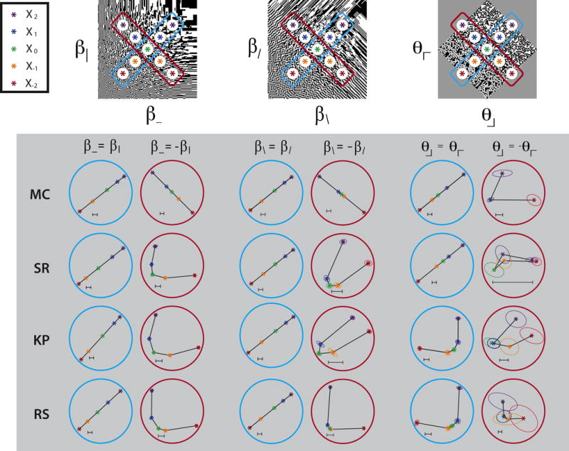
Multidimensional scaling of border salience judgments in selected coordinate planes in off-axis directions: cyan for same-sign directions, brown for opposite-sign directions. Other details as in Figure 8.

The low border saliences between points at the ends of the β_\ = −β_/ and θ_┘ = − θ_┌ -lines are not merely reflections of intrinsic properties of the stimulus space. More precisely, from the standpoint of an ideal observer that fully utilizes the image statistics, the similarity between image patches (measured by the Kullbach-Leibler divergence) increases monotonically. This holds not only in the on-axis directions studied in Figures 7 and 8, but also in the oblique directions studied in Figures 10 and 11. Thus, the low salience for borders between these points is a consequence of how these image statistics are processed and represented, and not due to intrinsic characteristics of the stimuli themselves.

The contrast between the off-axis results and findings for the on-axis datasets (Figure 8) is highlighted by quantification of the embedding analysis (Table 2). A one-dimensional embedding accounts for most of the judgments for on-axis test points, but not for test points in the off-axis directions in which the image statistics have opposite sign. This is seen from the normalized log-likelihood (see Methods) – a quantity that is zero for a model that is no better than chance, and one for a perfect model. For the on-axis datasets, the normalized log-likelihood is typically greater than 0.9 for the one-dimensional embedding. Two-dimensional models are not significantly better than one-dimensional models for any subject (γ and β_{_}), or for three of the four subjects (α), and when there is an improvement, the extent of the improvement is modest (~0.03 normalized log likelihood). In contrast, for test points along opposite-sign diagonals, a 2-dimensional model fit yields an improvement of at least this amount in 9 of the 12 datasets. The curvature associated with the two-dimensional fit shows the same contrast: for on-axis datasets, the ratio of the chord length (the distance between the first and last data points) and the arc length (the distance along the trajectory) ranges from 0.7 to 1.0, while along opposite-sign diagonals, 8 of 12 datasets have a ratio below 0.7.

We note that the poor fit of the 1-dimensional model and the consequent need for a two-dimensional curved locus in some datasets is unlikely to be a consequence of omitting a Weber- type component of subject uncertainty for comparing relative distances (see Methods). Specifically, this type of error would be expected to have a maximal impact in the datasets in which the compared distances are markedly suprathreshold (e.g., the directions γ, β_{_}, and β_{_} = β_|), and a minimal impact in which the compared distances are close to threshold (e.g., the direction θ_┘ = − θ_┌). However, Table 2 shows the opposite: a 1-dimensional embedding suffices when the compared distances are markedly suprathreshold and yields a good model fit (normalized log likelihood ratio typically > 0.95), but the 1-dimensional embedding fails when the distances are close to threshold (normalized log likelihood ratio < 0.6).

The uncertainty parameter σ (final columns of Table 2 and Figure 9) also shows very different behavior for the off-axis datasets, compared to the on-axis datasets. As mentioned above, for the on-axis datasets (Figure 9A), σ was nearly proportional to segmentation threshold. For the off-axis datasets (Figure 9B), σ had a much shallower dependence on segmentation threshold. Correspondingly, confidence intervals for the regression parameters of Figure 9A and B are non-overlapping (statistics given in figure legend).

To examine the dependence of σ on segmentation threshold in another way, we show the ratio of these quantities as a function of segmentation threshold in Figure 9C for both the on-axis and off-axis datasets. As expected from the near-proportionality seen in Figure 9A, the on-axis datasets form a horizontal band (solid symbols). In contrast, for the off-axis datsets (open symbols), σ is approximately constant, so the points lie on different trajectory. Quantitatively, for the prediction that the ratio of σ to segmentation threshold is constant within subjects, the unexplained variance is 0.0101 for the on-axis datasets, but 0.0632 for the off-axis datasets, a sixfold difference (p = 0.0013, two-tailed F-test, with 16 and 12 degrees of freedom).

Finally, although the above analysis ignores the non-uniformity of discrimination thresholds across the space, this non-uniformity is in the wrong direction to account for the results of the border salience experiment. The critical comparison is the β_\ = −β_/ dataset, since along this diagonal, systematic distortions are present in both experiments. In the segmentation experiments (Figure 6), thresholds increase modestly with increasing distance from the origin. This holds in all four subjects, as is manifest by the elongation of the magenta and lime-green contours towards the opposite-sign corners of the domain. If the same distortion were responsible for the trajectories in the border salience experiment (column 4 of Figure 11), then the perceptual distances between the peripherally-located point pairs (between ${\overrightarrow{x}}_2$ and ${\overrightarrow{x}}_1$ or between ${\overrightarrow{x}}_{-1}$ and ${\overrightarrow{x}}_{-2}$) should be less than the perceptual distances between the more centrally-located point pairs – since the peripheral pairs are harder to distinguish. But all four subjects show the opposite: the perceptual distances between the more peripherally-located pairs (purple to blue, yellow to red) are several times greater than for the more central ones (blue to green, or green to yellow).

Discussion

The broad aim of this work is to gain insight into how perceptual spaces are represented. We chose to study a perceptual space of visual textures, rather than a more familiar, classical space such as that of colors, because it has characteristics that are likely to be shared by perceptual spaces in general: it has a large number of dimensions, these dimensions are interdependent, and the dimensions are not simply related to the physical aspects of the stimulus. Within this space, we focused on a domain of textures consisting of black and white checks, parameterized by their local correlations. This is a 10-dimensional domain, large enough to capture the complexity of a general perceptual space and inter-relationships of natural image statistics (Hermundstad et al., 2014; Tkacik, Prentice, Victor, & Balasubramanian, 2010), but still tractable to probe explore extensively (Victor & Conte, 2012). To analyze how this space is represented, we examined threshold judgments (segmentation thresholds) and suprathreshold judgments (border salience). Our data show that to account for performance, two representations of the perceptual space are required.

Two independent lines of evidence lead to this conclusion. The first line of evidence is that the error patterns associated with the two kinds of tasks are incompatible, and thus, for these two tasks, the computations used to read out location in the stimulus domain must be different. If it were the case that judgments of segmentation thresholds and border salience were based on the same representation, then there should be a close relationship between performance on the two tasks. Specifically, the uncertainty in judging border salience in any direction of the texture space (the parameter σ, eq. (2)) should be proportional to the discrimination threshold in that direction, since both depend on the accuracy of locating a stimulus in the perceptual space. Figure 9 shows that this is not the case. Proportionality holds for the on-axis test directions (panel A), but the relationship breaks down in the off-axis directions (panel B). Consequently, the uncertainties determined from the two tasks do not obey a consistent relationship (panel C). However, while this discordance is readily quantifiable (a sixfold difference in variance explained between on-axis and off-axis directions, p < 0.002 via F-test), it gives no hint of the strategies employed to construct these representations or to read the distances out.

The second line of evidence is qualitative and only suggestive, but points to hypotheses for these strategies. The starting point is the observation that representing the stimulus space by brute force (e.g., with each distinguishable texture represented by its own set of neurons) is very demanding. We then recognize that there are two classes of combinatorial strategies that reduce the burden: a strategy that makes use of coordinates, and a distributed-representation strategy that does not. The coordinate-based approach readily accounts for the key features of the segmentation-threshold experiments, while the distributed strategy readily accounts for the key features of the border-salience experiments. We cannot rule out the possibility that the representation that underlies the segmentation-threshold experiments also uses a distributed strategy. However, the coordinate representation hypothesis is more parsimonious: it immediately accounts for the symmetry of thresholds in positive and negative directions, the approximate translation invariance of the isodiscrimination contours, and their elliptical shape. Known physiology is compatible with both strategies, and suggests a way in which the second strategy may build on the first.

How many textures can be distinguished?

To get a concrete idea of the representation problem that the brain has to solve, we can estimate the number of distinguishable visual textures. We first derive a conservative estimate confined to the stimulus space considered here, as it is can be directly linked to the subjects’ performance on the tasks we studied. This number, which is in the hundreds, indicates the minimal burden associated with a brute-force representation. But it is also a gross underestimate of the true burden of such a representation, since – as we detail below – there are many more dimensions of texture that we don’t even consider in this estimate.

To estimate the number of distinguishable textures in the present stimulus domain, we focus on the threshold experiments. We exploit the finding that within each plane, the isodiscrimination contours in the periphery are similar to those at the origin, both in their shape (Figures 4–6) and area (Table 1). Based on this, we consider the just-noticeable-difference (JND) for each texture coordinate to be constant throughout the plane. We choose the JND to be equal to the measured threshold on the segmentation task.

We can then estimate the number of distinguishable textures within each plane by computing the plane’s area, in units of square JND’s. This corresponds to filling the plane with a grid of points, spaced by the JND’s along each axis, an arrangement that guarantees that each point is at least one JND away from any other. For example, to estimate the number of distinguishable textures in the (β₋, β_|) plane, we first set the JND equal to the common threshold for β_{_} and β_| (Victor et al., 2015), here denoted a_β. We then note that the (β₋, β_|) plane itself covers the region −1 ≤ β_{_} ≤ 1 and −1 ≤ β_| ≤ 1, so it has an area of 4. Thus, in units of square JND’s, the plane has an area of 4 / (a_β²). For the four subjects in this study, the threshold a_β ranged from 0.25 to 0.32, yielding estimates of 38 to 62 discriminable textures in that plane. We computed a corresponding estimate for each image-statistic pair, taking into account that in many of the planes, the domain spanned by the two texture coordinates is less than a complete square (e.g., Figure 4A, see also (Victor & Conte, 2012)), and that the JND’s on each axis may differ. We then removed the duplicate counts that arose because the coordinate axes were each included in several planes, by subtracting the length of each axis (in JND’s) according to the number of extra times that it was counted. Across the four observers, this resulted in an estimate of 275 to 510 distinguishable textures within the 10-dimensional texture space.

This is a sizeable number, but nevertheless a severe underestimate of the number of textures that the visual system can distinguish. Even within the 10-dimensional texture space that is our focus, the estimate ignored any points that were not on the coordinate planes. But much more importantly, we ignored correlations at any scale beyond the specific check size used, and the further texture varieties that could be produced using oblique grids, gray levels, or colors. Thus, the actual number of distinguishable textures is likely to be much larger, probably by several orders of magnitude.

In terms of dimensionality, previous work showed that perceptual thresholds within the 10-dimensional texture space required nine independent perceptual dimensions (Victor et al., 2015). This too is likely to be a severe underestimate of the true number of perceptual dimensions used to encode all visual textures, as it also ignores scale, orientation, gray level, or color – all of which entail many further dimensions (Heeger, 1995; Portilla & Simoncelli, 2000; Saarela & Landy, 2012).

Avoiding a dimensional explosion with coordinates

Considering either the number or dimensionality of distinguishable textures, it seems unlikely that the brain uses a brute-force strategy to represent them, i.e., individual units dedicated to distinguishable stimuli. While a brute-force strategy is a simple one, the required resources grow exponentially with the number of perceptual dimensions: if N values are to be represented along each of D dimensions, then N^D individual units are required to represent each possible combination of values. Moreover, to allow for local statistical information to be used for segmentation, surface identification, etc., the neural representation of this domain needs be implemented repeatedly across visual space.

One strategy that avoids this dimensional explosion is to represent the domain in terms of coordinates. This is the strategy used for the representation of color, at least at the level of the lateral geniculate and primary visual cortex (Derrington et al., 1984; Lennie, Krauskopf, & Sclar, 1990). Since each coordinate is represented independently, the resources required grow in proportion to the number of dimensions, rather than exponentially. A coordinate representation could be realized in many ways, including an assignment of neurons to each distinguishable value along the coordinate axis, or, in analogy with color space, via opponent mechanisms (Derrington et al., 1984). Note also that the neural coordinates need not be identical to the coordinates used to define the stimulus domain, but rather, could be determined by some embedding of the stimulus domain into the neural representation. In all of these variations, the dimensional explosion is avoided because the space is represented in a combinatorial fashion.

A key aspect of a coordinate representation is that the perceptual distance between two stimuli is determined by the differences in coordinates that of the corresponding points. Specifically, suppose that Z is the embedding of the stimulus domain into the neural coordinates (i.e., that the stimuli $\overrightarrow{a}$ and $\overrightarrow{b}$ are represented by perceptual coordinates $\overrightarrow{A}=Z\left(\overrightarrow{a}\right)$ and $\overrightarrow{B}=Z\left(\overrightarrow{b}\right)$), and that f is the function that determines distance from the embedded coordinates. With this set-up, the perceptual distance between two points is given by

$$d\left(\overrightarrow{a},\overrightarrow{b}\right)=f\left(Z\left(\overrightarrow{a}\right)-Z\left(\overrightarrow{b}\right)\right).$$ (4)

We next ask to what extent this distance formula is consistent with experimental data. To constrain Z and f, we make use of previous work (Victor, Thengone, & Conte, 2013; Victor, Thengone, Rizvi, & Conte, 2015). Those studies characterized perceptual distances near the origin of the space, by determining thresholds to segment a structured texture from a random one. Distances near the origin were found to be given by a quadratic function of the coordinates of the stimulus domain:

$$d\left(\overrightarrow{x},0\right)=\sqrt{{\displaystyle \sum _{i,j}{Q}_{i,j}{x}_i{x}_j}},$$ (5)

where Q_i,._j, the elements of a symmetric matrix Q, were determined by the psychophysical data.

To use this result to test the hypothesis that the distances between two arbitrary points in the space are given by eq. (4), we first recast eq. (5) into the form of eq. (4). This can be done with

$$f\left(\overrightarrow{z}\right)=\left|\overrightarrow{z}\right|\mathit{and}Z\left(\overrightarrow{x}\right)=L\overrightarrow{x},$$ (6)

where L is a linear transformation from the coordinates of the stimulus domain to the neural that satisfies

$$L^{T}L=Q.$$ (7)

(The existence of such an L is guaranteed because Q is symmetric and non-negative definite.). As is well-known(Poirson, Wandell, Varner, & Brainard, 1990), we note that eq. (7) only determines L up to orthogonal transformation – but this does not bear on the predictions made by eq. (4), since they only depend on Q:

$$\begin{gathered} d\left(\overrightarrow{a},\overrightarrow{b}\right)=f\left(Z\left(\overrightarrow{a}\right)-Z\left(\overrightarrow{b}\right)\right)=\left|L\overrightarrow{a}-L\overrightarrow{b}\right| \\ =\left|L\left(\overrightarrow{a}-\overrightarrow{b}\right)\right|=\sqrt{{\left(L\left(\overrightarrow{a}-\overrightarrow{b}\right)\right)}^{T}L\left(\overrightarrow{a}-\overrightarrow{b}\right)} \\ =\sqrt{{\left(\overrightarrow{a}-\overrightarrow{b}\right)}^T{L}^{T}L\left(\overrightarrow{a}-\overrightarrow{b}\right)}=\sqrt{{\left(\overrightarrow{a}-\overrightarrow{b}\right)}^{T}Q\left(\overrightarrow{a}-\overrightarrow{b}\right)}. \end{gathered}$$ (8)

In geometric terms, the above algebra takes the finding of (Victor et al., 2013; Victor et al., 2015) – that perceptual distances are given by the Euclidean distance in a space that is a linear transformation of the stimulus domain – and hypothesizes that it applies not only near the origin, but throughout the space.

If this hypothesis holds, then isodiscrimination contours at peripherally-located reference points, as measured in the segmentation experiments, should be identical in size and shape to the isodiscrimination points at the origin. To a first approximation, this holds. However, inspection of Figures 4–6 show that there are systematic differences in the peripherally-located isodiscrimination contours, compared to the corresponding contours at the origin. These distortions rule out the hypothesis that the embedding Z is strictly linear, and suggest that a refinement in which it is replaced by a nonlinear embedding that captures the distortions of the isodiscrimation contours. Note that a globally nonlinear embedding still predicts that the isodiscrimination contours will be elliptical, provided that the nonlinearity is gentle enough so that in local regions, it can be approximated by a linear embedding –but the elliptical contours won’t all be the same size and shape.

A mildly nonlinear embedding combined with quadratic combination of perceptual coordinates also accounts for findings in other domains – for example, the ellipsoidal isodiscrimination contours in color space and the change in the size of these contours across the space (Macadam, 1942; Poirson et al., 1990), and the perceptual combination of color and orientation cues (Saarela & Landy, 2012).

However, a mildly nonlinear embedding does not readily account for the border salience data. The reason for the failure is that along some directions (especially the β_\ = −β_/ and θ_┘ = − θ_┌ directions), points that are at opposite ends in the stimulus domain are perceptually closer to each other than they are to the origin (Figure 11). Accounting for this behavior requires an embedding of a different character: the nonlinearity has to be sufficiently strong so as to map opposite ends of the stimulus domain to nearby points in the internal representation. A nonlinearity of this type is not suggested by the threshold data, but we cannot completely exclude it. The reason is that the points that demonstrated this “wraparound” behavior in the border salience experiments were either too close to the edge of the stimulus domain to measure the surrounding isodiscrimination contours (in the β_\ = −β_/ case), or directly on the edge of the space (in the case of θ_┘ = − θ_┌.

Avoiding a dimensional explosion without coordinates

While a coordinate-based representation accounts for the wraparound behavior seen in the border salience data only if coupled with a strong nonlinearity, a different kind of representation will lead to this behavior in a more natural way. Consider instead a representation based on neurons that respond to blob-like regions of the stimulus domain. We hypothesize that these coding regions – essentially, “receptive fields” in the stimulus domain – are large, blob-like, and randomly-placed, and hence overlap in a haphazard but extensive fashion. Similarity relationships can be directly read out from the population response without an intermediate step of computing coordinates, or even knowing the location of each neuron’s receptive field in the stimulus domain: two stimuli are similar if they induce similar patterns of population activity. Two stimuli that correspond to nearby points will be regarded as similar, since they activate a similar pattern of neurons, and neurons that correspond to distant points will be regarded as different, since the pattern of activated neurons will differ. We emphasize that the key distinction between this kind of representation and the coordinate strategy is not whether neurons are linear vs. nonlinear, but rather, whether they have location labels that are needed to determine perceptual distances.

This coding strategy is combinatorial because the coding regions are large and extensively overlapping: stimulus identity is coded by the combination of neurons whose coding regions cover a given point in the domain. The combinatorial character would be lacking if the coding regions were narrowly tuned and had minimal overlap. In this case, stimulus location could be coded by the identity of the active neuron, but the entire space would need to be covered by separate coding regions, so the combinatorial advantage would be lost. This intuition is supported by theoretical studies: while the ability of a population of neurons to represent the location of points within a multidimensional domain depends on many factors, including the size of each neuron’s coding region, the extent to which these coding regions overlap, the slopes of their tuning functions, and whether they have correlated or uncorrelated noises (Hinton, McClelland, & Rumelhart, 1986; Zhang & Sejnowski, 1999), broader tuning curves provide a more efficient representation than narrow ones for spaces of dimension three or larger (Zhang & Sejnowski, 1999). We also note that a similar combinatorial advantage emerges in a distributed representation based on neurons with periodic coding regions at multiple scales, as in the grid cell system (Mathis, Herz, & Stemmler, 2012; Mathis, Stemmler, & Herz, 2015).

The wraparound observed in the border salience experiments will occur whenever there are regions near the periphery of the stimulus space that are only sparsely covered by coding regions. The reason for this is that stimuli placed in these sparsely-covered regions will activate very few neurons, so all such stimuli will appear similar to each other. This is in contrast to similar located in densely-covered regions, which will differentially activate large numbers of neurons.

An uneven coverage of the stimulus domain studied here, with greater resources devoted to the region near the origin, makes sense in terms of efficient coding: the 2× 2 statistics of natural image patches rarely populate the periphery of the space (Hermundstad et al., 2014). This account of the curvature of the trajectories in Figure 11 is also consistent with more detailed aspects of the distribution of 2× 2 natural image statistics in the planes considered here. Specifically, the distribution of statistics of natural image patches falls off more rapidly in the opposite-sign directions than in the same-sign directions, consistent with the observation that curvatures are more prominent in opposite-sign directions than in same-sign directions (Fig. 3B of Hermundstad et al., 2014). That analysis further shows that within the opposite-sign directions, the fall-off of image statistics is most rapid for θ_┘ = − θ_┌, next for β_\ = −β_/, and least for β_{_} = −β_| – corresponding to the relative prominence of curvature of the trajectories in Figure 11. It is also notable that the distribution of values of α in natural images has a strong positive skew (Supplementary Figure 3A of (Hermundstad et al., 2014); Supplementary Figure 10 of (Tkacik et al., 2010)). The compression of the trajectories for negative values of α seen in Figure 8 (column 5) indicates a correspondingly sparser representation of the space for α < 0 compared to α > 0. While the directions of greatest curvature correspond to the directions in which natural image statistics fall off most rapidly, it is unlikely that coding units are strictly distributed in proportion to the occurrence of the corresponding image statistics in natural images. A further analysis of the data in (Hermundstad et al., 2014) (provided by the first author) suggests that the periphery of the domain is over-represented, compared to the distribution of image statistics in natural image patches. In natural image patches, the standard deviation for the cardinal β’s (β_{_} and β_|) is < 0.12, for the diagonal β’s (β_\ and β_/) it is 0.08, for θ it is < 0.04, and for α it is < 0.05. A distribution of coding regions proportional to the natural image distribution would not account for the observation that the most distinguishable pair of test points in the on-axis experiments was ${\overrightarrow{x}}_{-2}$ and ${\overrightarrow{x}}_2$

(Figure 8), as these endpoints are each four or more standard deviations from the peak of the natural image distribution.

A distributed representation based on coding regions may also explain the relatively poor fit of eq. (2) for the test points along θ_┘ = − θ_┌. For these datasets, the typical relative log likelihood was approximately 0.5 (last section of Table 2) for a two-dimensional embedding, and there was no improvement with a higher-dimensional embedding. This lack of improvement indicates that the perceptual distances are inconsistent with a Euclidean distance, no matter how the stimulus coordinates are transformed. However, distributed representations allow for non-Euclidean distances: the difference in the patterns of population activity need not be computed in a quadratic fashion. For example, the distance may correspond to the sum of the differences in firing rates, rather than the square root of the sum of the squares. Comparisons of multineuronal activity patterns based on spike timing are also typically non-Euclidean (Aronov & Victor, 2004).

Finally, independent of the evidence from the analysis of error patterns (Figure 9), there are additional reasons that a single distributed representation is unlikely to account for both the segmentation thresholds and border salience. First, in order for this kind of representation to account for the near-uniformity of the isodiscrimination contours, coding regions would need to be distributed approximately uniformly throughout the space, implying extensive allocation of resources to image statistics that are very rare in natural images. Further evidence against a common representation emerges from a direct comparison of the two tasks carried out in the planes of the second-order statistics (β_{_}, β_|) and (β_\, β_/). We focus on the behavior in the neighborhood of the intermediate test points ( ${\overrightarrow{x}}_{-1}$ and ${\overrightarrow{x}}_1$) used in the border salience task along the difference direction; these are at locations (±0.25, ∓0.25). The border salience experiments (Figure 11, second and fourth columns) showed that the perceptual distances from each of these points to the corresponding extreme point (i.e,. from ${\overrightarrow{x}}_1$ (blue) to ${\overrightarrow{x}}_2$ (purple), or from ${\overrightarrow{x}}_{-1}$ (yellow) to ${\overrightarrow{x}}_{-2}$ (red)) were typically more than twice their perceptual distances to the origin ( ${\overrightarrow{x}}_0$, green). If threshold judgments were based on the same representation, thresholds should be about half as large for steps away from the origin, compared to steps towards it. However, direct measurements of threshold at peripheral locations ((β_{_}, β_|) = (±0.6, ∓0.6) and (β_\, β_/) = (±0.35, ∓0.35)) show no corresponding asymmetry (Figures 5 and 6; Table 1) – there is either no asymmetry at all, or a mild asymmetry in the wrong direction (a larger threshold when moving away from the origin, than towards it). In sum, the asymmetries seen in the border salience task are inconsistent with the near-constancy of the isodiscrimation contours obtained in the threshold experiments.

Physiological implications

What plausible neural mechanisms could account for our findings? Recordings in macaque V1 and V2 (Yu, Schmid, & Victor, 2015) (Victor, Yu, Thengone, Witztum, Nitzany, and Purpura, 2015) under anesthesia identify neurons sensitive to local image statistics of all orders in both regions, with V2 containing a much larger proportion of neurons sensitive to third-and fourth-order statistics. In both V1 and V2, responses depended on the value of an image statistic in a monotonic though often nonlinear fashion (Victor, Yu, Thengone, Witztum, Nitzany, and Purpura, 2015). These neurons, while not providing strictly linear coordinates, may nevertheless form the substrate of a coordinate representation. Individual neurons tended to respond to more than one image statistic, and their responses were not restricted to a specific set of coordinate axes, suggesting that the representation is overcomplete. These features are shared by the representation of color space in V1: neurons typically respond in a partially rectified manner to modulations along a preferred axis in color space, and across the population, these preferred axes are not restricted to a set of cardinal axes (Lennie et al., 1990).

On the other hand, neurons whose activity could account for the border salience findings need to have responses that depend on stimulus coordinates in a non-monotonic fashion. A monotonic relationship to the domain coordinates is ruled out because in that case, the perceptual distances between two points would grow monotonically as a function of their distance along the coordinate axes – the opposite of what is observed (Figure 11: along the β_\ = −β_/ and θ_┘ = − θ_┌ -lines). In the context of a coding-region representation, non-monotonicity is also required, because the neuron’s response is maximal for stimuli that lie within this “coding region”, and falls off to small values for stimuli that are outside of it. However, neurons with non-monotonic responses were rarely identified in the above studies. We hypothesize that non-monotonicity could emerge by combining the outputs of neurons with monotonic responses – either by a nonlinear interaction, or simply by subtracting the output of neurons whose response functions have different shapes. In this scenario, even though the neural basis for threshold and suprathreshold judgments are distinct, they share common building blocks. Interestingly, non-monotonic neuronal response functions, and an analogous patch-like representation of color space, have been observed in macaque inferotemporal cortex (Komatsu, Ideura, Kaji, & Yamane, 1992).

While there appear to be a number of parallels between image statistics and color, it is worth noting that there are a number of important differences, beyond just differences in dimensionality. The stimulus domains are fundamentally different: for color, the space is affine, i.e., there is no a priori notion of a distance (Zaidi et al., 2013); for image statistics, information-theoretic considerations give the space an intrinsic metrical structure (Victor & Conte, 2012). For color, the parameters of the perceptual space are extracted by the photoreceptors and determined by the spectra of photopigments, while for image statistics, they are extracted at many levels of processing and determined by the computational characteristics of neural circuitry. Finally, the partitioning of color space into categories or regions with specific names, and the likely substrate of this partitioning in neural processing (Komatsu, 1998; Komatsu et al., 1992), have no obvious analogy for image statistics.

Conclusions

Representing a perceptual space by brute force requires resources that grow exponentially with the number of dimensions. Representations based on coordinate axes or coding regions avoid this exponential growth because they are essentially combinatorial. The present data indicate that for image statistics, there are separate representations that support segmentation tasks near threshold, and suprathreshold comparisons. The former has characteristics suggestive of a coordinate-based representation, while the latter has characteristics suggestive of a representation in terms of coding regions. There is evidence that similar strategies are used for color – leading to the speculation that they are used more generally for the representation of complex, multidimensional perceptual spaces. How these representations are interrogated in a task-dependent fashion, and how they are implemented in neural circuitry, remain for future work.

Significance Statement.

To move from sensory signals to decisions and actions, the brain carries out a sequence of transformations. An important stage in this process is the construction of a “perceptual space” – an internal workspace of sensory information that captures similarities and differences, and enables further processing, such as classification and naming. Perceptual spaces for color, faces, visual and haptic textures and shapes, sounds, and odors (among others) are known to exist. How such spaces are represented is at present unknown. Here, using visual textures as a model, we investigate this. Psychophysical measurements suggest roles for two combinatorial strategies: one based on projections onto coordinate-like axes, and one based on patterns of activity across broadly tuned elements scattered throughout the space.

References

- Aronov D, Victor JD. Non-Euclidean properties of spike train metric spaces. Phys Rev E Stat Nonlin Soft Matter Phys. 2004;69(6 Pt 1):061905. doi: 10.1103/PhysRevE.69.061905. [DOI] [PMC free article] [PubMed] [Google Scholar]
- Baylor DA, Nunn BJ, Schnapf JL. Spectral sensitivity of cones of the monkey macaca fascicularis. J Physiol (Lond) 1987;390:145–160. doi: 10.1113/jphysiol.1987.sp016691. [DOI] [PMC free article] [PubMed] [Google Scholar]
- Bushdid C, Magnasco MO, Vosshall LB, Keller A. Humans can discriminate more than 1 trillion olfactory stimuli. Science. 2014;343(6177):1370–1372. doi: 10.1126/science.1249168. [DOI] [PMC free article] [PubMed] [Google Scholar]
- Catz O, Kampf M, Nachson I, Babkoff H. From theory to implementation: building a multidimensional space for face recognition. Acta Psychol (Amst) 2009;131(2):143–152. doi: 10.1016/j.actpsy.2009.03.010. [DOI] [PubMed] [Google Scholar]
- Chubb C, Landy MS, Econopouly J. A visual mechanism tuned to black. Vision Res. 2004;44(27):3223–3232. doi: 10.1016/j.visres.2004.07.019. [DOI] [PubMed] [Google Scholar]
- Cho RY, Yang V, Hallett PE. Reliability and dimensionality of judgments of visually textured materials. Percept Psychophys. 2000;62(4):735–752. doi: 10.3758/bf03206920. [DOI] [PubMed] [Google Scholar]
- Derrington AM, Krauskopf J, Lennie P. Chromatic mechanisms in lateral geniculate nucleus of macaque. J Physiol. 1984;357:241–265. doi: 10.1113/jphysiol.1984.sp015499. [DOI] [PMC free article] [PubMed] [Google Scholar]
- Doi E, Balcan DC, Lewicki MS. Robust coding over noisy overcomplete channels. IEEE Trans Image Process. 2007;16(2):442–452. doi: 10.1109/tip.2006.888352. [DOI] [PubMed] [Google Scholar]
- Edelman S. Representation is the representation of similarities. Behav Brain Sci. 1998;21(4):449–467. doi: 10.1017/s0140525x98001253. [DOI] [PubMed] [Google Scholar]
- Freiwald WA, Tsao DY, Livingstone MS. A face feature space in the macaque temporal lobe. Nat Neurosci. 2009;12(9):1187–1196. doi: 10.1038/nn.2363. [DOI] [PMC free article] [PubMed] [Google Scholar]
- Gaissert N, Wallraven C, Bulthoff HH. Visual and haptic perceptual spaces show high similarity in humans. J Vis. 2010;10(11):2. doi: 10.1167/10.11.2. [DOI] [PubMed] [Google Scholar]
- Geffen MN, Gervain J, Werker JF, Magnasco MO. Auditory perception of self-similarity in water sounds. Front Int Neurosci. 2011;5:15. doi: 10.3389/fnint.2011.00015. [DOI] [PMC free article] [PubMed] [Google Scholar]
- Heeger DJ, Bergem JR. SIGGRAPH ’95 Proceedings of the 22nd Annual Conference on Computer Graphics and Interactive Techniques. New York: ACM; 1995. Pyramid-based texture analysis/synthesis; pp. 229–238. [Google Scholar]
- Hermundstad AM, Briguglio JJ, Conte MM, Victor JD, Balasubramanian V, Tkacik G. Variance predicts salience in central sensory processing. Elife. 2014;3 doi: 10.7554/eLife.03722. [DOI] [PMC free article] [PubMed] [Google Scholar]
- Hinton GE, McClelland JL, Rumelhart DE. Distributed representations. In: Rumelhart DE, McClelland JL, editors. Parallel distributed processing. Cambridge, MA: MIT Press; 1986. pp. 77–109. [Google Scholar]
- Julesz B. Visual pattern discrimination. IRE Trans Inf Theory(IT-8) 1962:84–92. [Google Scholar]
- Julesz B. Textons, the elements of texture perception, and their interactions. Nature. 1981;290(5802):91–97. doi: 10.1038/290091a0. [DOI] [PubMed] [Google Scholar]
- Julesz B, Gilbert EN, Shepp LA, Frisch HL. Inability of humans to discriminate between visual textures that agree in second-order statistics–revisited. Perception. 1973;2(4):391–405. doi: 10.1068/p020391. [DOI] [PubMed] [Google Scholar]
- Julesz B, Gilbert EN, Victor JD. Visual discrimination of textures with identical third-order statistics. Biol Cybern. 1978;31(3):137–140. doi: 10.1007/BF00336998. [DOI] [PubMed] [Google Scholar]
- Knoblauch K, Maloney LT. Estimating classification images with generalized linear and additive models. J Vis. 2008;8(16):10 11–19. doi: 10.1167/8.16.10. [DOI] [PMC free article] [PubMed] [Google Scholar]
- Komatsu H. Mechanisms of central color vision. Current Biology. 1998;8(8):503–508. doi: 10.1016/s0959-4388(98)80038-x. [DOI] [PubMed] [Google Scholar]
- Komatsu H, Ideura Y, Kaji S, Yamane S. Color selectivity of neurons in the inferior temporal cortex of the awake macaque monkey. J Neurosci. 1992;12(2):408–424. doi: 10.1523/JNEUROSCI.12-02-00408.1992. [DOI] [PMC free article] [PubMed] [Google Scholar]
- Koulakov AA, Kolterman BE, Enikolopov AG, Rinberg D. In search of the structure of human olfactory space. Front Syst Neurosci. 2011;5:65. doi: 10.3389/fnsys.2011.00065. [DOI] [PMC free article] [PubMed] [Google Scholar]
- Lennie P, Krauskopf J, Sclar G. Chromatic mechanisms in striate cortex of macaque. J Neurosci. 1990;10(2):649–669. doi: 10.1523/JNEUROSCI.10-02-00649.1990. [DOI] [PMC free article] [PubMed] [Google Scholar]
- Macadam DL. Visual sensitivities to color differences in daylight. Journal of the Optical Society of America. 1942;32:247–273. [Google Scholar]
- Maloney LT, Yang JN. Maximum likelihood difference scaling. J Vis. 2003;3(8):573–585. doi: 10.1167/3.8.5. [DOI] [PubMed] [Google Scholar]
- Mathis A, Herz AV, Stemmler M. Optimal population codes for space: grid cells outperform place cells. Neural Comput. 2012;24(9):2280–2317. doi: 10.1162/NECO_a_00319. [DOI] [PubMed] [Google Scholar]
- Mathis A, Stemmler MB, Herz AV. Probable nature of higher-dimensional symmetries underlying mammalian grid-cell activity patterns. Elife. 2015;4 doi: 10.7554/eLife.05979. [DOI] [PMC free article] [PubMed] [Google Scholar]
- Maxwell JC. On the theory of compound colours and the relations of the colours of the spectrum. Phil Trans Roy Soc. 1860;150:57–84. [Google Scholar]
- McDermott JH, Schemitsch M, Simoncelli EP. Summary statistics in auditory perception. Nat Neurosci. 2013;16(4):493–498. doi: 10.1038/nn.3347. [DOI] [PMC free article] [PubMed] [Google Scholar]
- McDermott JH, Simoncelli EP. Sound texture perception via statistics of the auditory periphery: evidence from sound synthesis. 2011 doi: 10.1016/j.neuron.2011.06.032. [DOI] [PMC free article] [PubMed] [Google Scholar]
- Poirson A, Wandell B, Varner D, Brainard D. Surface characterizations of color thresholds. J Opt Soc Am. 1990;A7:783–789. doi: 10.1364/josaa.7.000783. [DOI] [PubMed] [Google Scholar]
- Portilla J, Simoncelli EP. A parametric texture model based on joint statistics of complex wavelet coefficients. International Journal of Computer Vision. 2000;40(1):49–71. [Google Scholar]
- Saarela T, Landy MS. Combination of texture and color cues in visual segmentation. Vision Res. 2012;58:59–67. doi: 10.1016/j.visres.2012.01.019. [DOI] [PMC free article] [PubMed] [Google Scholar]
- Tanaka JW, Meixner TL, Kantner J. Exploring the perceptual spaces of faces, cars and birds in children and adults. Devel Sci. 2011;14(4):762–768. doi: 10.1111/j.1467-7687.2010.01023.x. [DOI] [PMC free article] [PubMed] [Google Scholar]
- Tkacik G, Prentice JS, Victor JD, Balasubramanian V. Local statistics in natural scenes predict the saliency of synthetic textures. Proc Natl Acad Sci U S A. 2010;107(42):18149–18154. doi: 10.1073/pnas.0914916107. [DOI] [PMC free article] [PubMed] [Google Scholar]
- Valentine T. A unified account of the effects of distinctiveness, inversion, and race in face recognition. Q J Exp Psychol A. 1991;43(2):161–204. doi: 10.1080/14640749108400966. [DOI] [PubMed] [Google Scholar]
- Victor JD, Chubb C, Conte MM. Interaction of luminance and higher-order statistics in texture discrimination. Vision Res. 2005;45(3):311–328. doi: 10.1016/j.visres.2004.08.013. [DOI] [PubMed] [Google Scholar]
- Victor JD, Conte MM. Local image statistics: maximum-entropy constructions and perceptual salience. J Opt Soc Am A Opt Image Sci Vis. 2012;29(7):1313–1345. doi: 10.1364/JOSAA.29.001313. [DOI] [PMC free article] [PubMed] [Google Scholar]
- Victor JD, Thengone DJ, Conte MM. Perception of second- and third-order orientation signals and their interactions. J Vis. 2013;13(4):21. doi: 10.1167/13.4.21. [DOI] [PMC free article] [PubMed] [Google Scholar]
- Victor JD, Thengone DJ, Rizvi SM, Conte MM. A perceptual space of local image statistics. Vision Res. 2015;117:117–135. doi: 10.1016/j.visres.2015.05.018. [DOI] [PMC free article] [PubMed] [Google Scholar]
- Victor JD, Yu Y, Thengone DJ, Witztum J, Nitzany EI, Purpura KP. Society for Neuroscience 2015 Program no. 332.15. Washington, DC: Society for Neuroscience; 2015. How do neurons in macaque visual cortex represent a high-dimensional perceptual space? (Neuroscience Meeting Planner). 2015. [Google Scholar]
- Wallraven C. Touching on face space: Comparing visual and haptic processing of face shapes. Psychonomic Bulletin Review. 2014 doi: 10.3758/s13423-013-0577-y. [DOI] [PubMed] [Google Scholar]
- Weisstein EW. Likelihood Ratio–A Wolfram. 2016 Web Resource from http://mathworld.wolfram.com/LikelihoodRatio.html.
- Wolfson SS, Landy MS. Examining edge- and region-based texture analysis mechanisms. Vision Res. 1998;38:439–446. doi: 10.1016/s0042-6989(97)00153-3. [DOI] [PubMed] [Google Scholar]
- Yoshioka T, Bensmaia SJ, Craig JC, Hsiao SS. Texture perception through direct and indirect touch: an analysis of perceptual space for tactile textures in two modes of exploration. Somatosens Mot Res. 2007;24(1-2):53–70. doi: 10.1080/08990220701318163. [DOI] [PMC free article] [PubMed] [Google Scholar]
- Yu Y, Schmid AM, Victor JD. Visual processing of informative multipoint correlations arises primarily in V2. Elife. 2015;4 doi: 10.7554/eLife.06604. [DOI] [PMC free article] [PubMed] [Google Scholar]
- Zaidi Q, Victor J, McDermott J, Geffen M, Bensmaia S, Cleland TA. Perceptual spaces: mathematical structures to neural mechanisms. J Neurosci. 2013;33(45):17597–17602. doi: 10.1523/jneurosci.3343-13.2013. [DOI] [PMC free article] [PubMed] [Google Scholar]
- Zhang K, Sejnowski TJ. Neuronal tuning: To sharpen or broaden? Neural Comput. 1999;11(1):75–84. doi: 10.1162/089976699300016809. [DOI] [PubMed] [Google Scholar]
Associated Data
This section collects any data citations, data availability statements, or supplementary materials included in this article.