Dirichlet Process Mixture Model for Correcting Technical Variation in Single-Cell Gene Expression Data

Abstract

We introduce an iterative normalization and clustering method for single-cell gene expression data. The emerging technology of single-cell RNA-seq gives access to gene expression measurements for thousands of cells, allowing discovery and characterization of cell types. However, the data is confounded by technical variation emanating from experimental errors and cell type-specific biases. Current approaches perform a global normalization prior to analyzing biological signals, which does not resolve missing data or variation dependent on latent cell types. Our model is formulated as a hierarchical Bayesian mixture model with cell-specific scalings that aid the iterative normalization and clustering of cells, teasing apart technical variation from biological signals. We demonstrate that this approach is superior to global normalization followed by clustering. We show identifiability and weak convergence guarantees of our method and present a scalable Gibbs inference algorithm. This method improves cluster inference in both synthetic and real single-cell data compared with previous methods, and allows easy interpretation and recovery of the underlying structure and cell types.

1. Introduction

Single-cell RNA-seq (scRNA-seq) is a recent breakthrough technology that measures gene expression at the resolution of individual cells (Hashimshony et al., 2012; Jaitin et al., 2014; Shalek et al., 2013) presenting exciting opportunities to study heterogeneity of expression and characterize unknown cell types. This contrasts traditional bulk gene expression data where the gene expression is measured by an average readout across a bulk of cells.

Analyzing scRNA-seq measurements involves many challenges, including the fact that the data is only one sample set from the transcriptome (the full range of mRNAs representing gene expression) with high chances of missing low-expression genes termed as dropouts¹, biases in cell sampling, significant differences in total number of mRNA molecules, as well as variation in library size, defined as sum of amplified mRNA molecules per cell (Kharchenko et al., 2014). These cell type-specific biases can not be resolved with common normalization techniques designed for bulk RNA-seq data. Global normalization by median library size (Oshlack et al., 2010) or through spike-ins² (Vallejos & Richardson, 2015) would not resolve dropouts, and can lead to spurious differential expression or removal of biological stochasticity specific to each cell type, both of which induce improper clustering and characterization of latent cell types. Thus, normalization prior to clustering fails to consider cell type dependent technical variation, and the cell types are not known a priori, hence the normalization and clustering become a chicken- and-egg problem.

To address this problem, we model biological and technical variation in parallel, which we refer to as BISCUIT (Bayesian Inference for Single-cell ClUstering and ImpuTing). This is done through incorporating parameters denoting technical variation into a Hierarchical Dirichlet Process mixture model (HDPMM). This allows inference of clusters of cells based on similar gene expression and identifies technical variation per cell. Furthermore, this model can be leveraged to impute dropouts and normalize data based on cells with similar co-expression patterns. This simultaneous recovery of clusters and associated technical variations is a step-up from previous methods that infer the variations in a decoupled manner.

Although this model is motivated by challenges in scRNA-seq data, BISCUIT could also be applied to other domains where clusters are subject to different variation. One example is in stock markets where stock prices associated with certain time periods can fluctuate much more than calmer periods (Lamoureux & Lastrapes, 1990). Investing in a highly unstable period leads to potential monetary loss and thus clustering periods of high and low price fluctuations will help to better forecast stock prices and aid investments. In these cases, approaches that do not consider heteroscedasticity can result in spurious clustering due to erroneous distributional assumptions.

In the next section we highlight the importance of addressing this problem in the single-cell domain and motivate the structure of our model based on observations. The model is elaborated in Section 3 with theoretical guarantees in Section 4. In Section 5, we present the scalable Gibbs inference algorithm. Results are demonstrated in Section 6 followed by concluding remarks in Section 7.

2. Preliminaries of single-cell data and biological motivation

Akin to the remarkable efforts in the development of DNA sequencing methods that built maps of genomes, recent advances in scRNA-sequencing now give the opportunity for building an atlas of cells through characterizing mixtures of previously unknown cell types and functions in tissues (Di Palma & Bodenmiller, 2015; Navin, 2014; Junker & van Oudenaarden, 2014; Gawad et al., 2014; Paul et al., 2015).

However, to characterize these cell types, clustering methods applied to scRNA-seq data commonly perform a single global normalization that is invariant to cell types, leading to the undesired consequence of grouping cells due to technical artifacts rather than true biology. Currently, there is a dearth of robust clustering algorithms that distinguish technical variation from biological signal in scRNA-seq data.

A number of characteristics of this data confound clustering: 1. Typical scRNA-seq datasets involve a significant number of dropouts in low expression genes, which should ideally be imputed for downstream analysis. 2. Multiple rounds of exponential amplification needed to generate adequate library for sequencing can have different effects on different latent cell types and cause a heavy-tail distribution of library size, suggesting over-dispersed data (Figure 1). 3. The data are also prone to high levels of technical variation due to differences in machine, enzyme activity, lysis efficiency or experimental protocol. Factoring in and correcting for this variation are some of the key challenges in analyzing scRNA-seq data (Brennecke et al., 2013; Stegle; Kharchenko et al., 2014). BISCUIT is the first method to simultaneously correct these technical artifacts (without needing spike-in genes) and infer clusters of cells based on gene co-expression patterns. We demonstrate that such inference is superior to first normalizing and then clustering in a decoupled manner.

Figure 1.

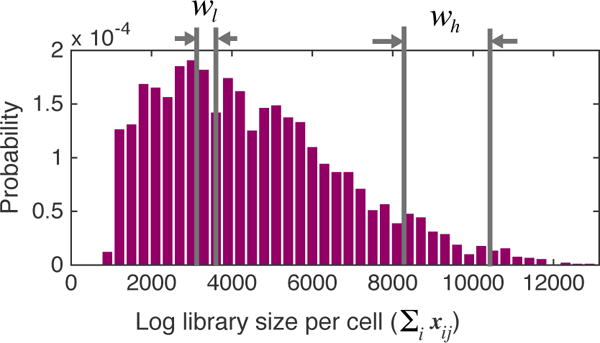
Distribution of log library size in an example scRNA-seq dataset (Zeisel et al., 2015). The heavy tail is indicative of over-dispersion in data. Two windows of cells with low and high library size are selected for motivating cell-specific scaling in Section 2.

Notations

We begin with a single-cell expression matrix X_d×n with n single-cell observations {x₁, x₂, …, x_n} where each observation x_j ∈ ℝ^d corresponds to·d·genes (as features). Each entry x_ij contains the log of counts of mRNA molecules per gene i from cell j plus one (or a pseudo-count), which represents the expression of gene i in cell j. X is typically extremely sparse. Zeros may represent gene dropouts or true lack of expression. The log library size per cell j, given as ${\displaystyle {\sum }_{i=1}^d{x}_{ij}}$, is highly variable (Figure 1). In an ideal setting with no technical variation, the library size for all cells would be roughly the same. Thus it is imperative to denoise the data by correcting for these technical variations, for downstream analysis.

Motivation for cell-specific scalings

To analyze the effects of technical variation, we studied an example single-cell dataset containing 3005 cells (Zeisel et al., 2015). We chose 150 cells from a window with high library size (w_h in Figure 1) and 150 cells from another window with low library size (w_l). The means and variances of every gene i across cells in the high library size window is given by ${\mu }_h^{\left(i\right)}={\mathbb{E}}_{j\in w_h}\left\{x_{ij}\right\}$ and ${\sigma }_h^{2\left(i\right)}=Va{r}_{j\in w_h}\left\{x_{ij}\right\}$ and similarly across the low library size as ${\mu }_l^{\left(i\right)}={\mathbb{E}}_{j\in w_l}\left\{x_{ij}\right\}$ and ${\sigma }_l^{2\left(i\right)}=Va{r}_{j\in w_l}\left\{x_{ij}\right\}$. Figure 2 (top) indicates a correlation structure between μ_h and μ_l and also between ${\sigma }_h^2$ and ${\sigma }_l^2$. If we select a particular known cluster of cells, e.g. interneuronal cells in each window, and condition μs and σ²s on this cluster, we see a pronounced linear relationship especially between means (Figure 2, bottom) suggesting linear scaling of moments of expression of all genes per cell with the same factor. Hence, for cells in w_h we define $\alpha :{\mu }_h^{\left(i\right)}/{\mu }_l^{\left(i\right)}$ and $\beta :={\sigma }_h^{2\left(i\right)}/{\sigma }_l^{2\left(i\right)}$ for all i, which can be related to amplification rate of each cell (cells in the same window have more or less the same amplification). Since a clear dependence structure is not discernible between α, β (Figure S1), this encouraged modeling them as separate parameters for cell-specific moment-scaling.

Figure 2.

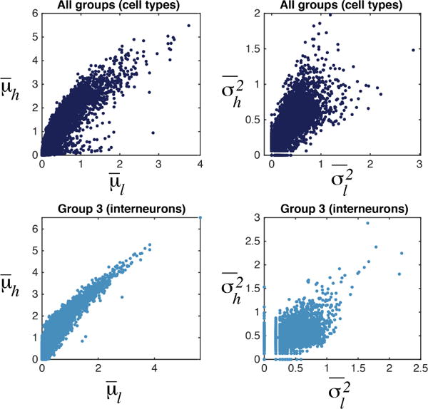
Top: Means and variances per gene across a window of cells with high library size vs a window of cells with low library size (each data point is one gene). Bottom: Same for a particular cluster (cell type): interneurons.

2.1. Related work

There have been previous attempts to separate biological variability from technical variation in single-cell expression data. Kharchenko et al. (2014) assumes gene counts per cell to be generated from a mixture of zero-inflated Poisson for dropouts and a negative-binomial for detected and amplified genes. This model neither considers cell-type-dependent variation nor infers clusters. Jaitin et al. (2014) normalizes the data based on a total count threshold per cell and down-samples cells with counts greater than the threshold whilst removing cells with lesser counts. The data is modeled as a mixture of multinomials with an EM-like inference. Drawbacks here are discarding majority of data with down-sampling/filtering, cell type-independent correction and EM-related local optima issues.

Similarly, Brennecke et al. (2013) and Buettner et al. (2015) resort to an initial weighted mean normalization based on each cell’s library size (total counts). While this normalization does not introduce significant noise in bulk sequencing techniques (Anders & Huber, 2010), it is detrimental to heterogeneous and sparse single-cell data. Cells with small library size have many zero entries (dropouts); a strong bias that remains after library-size scaling.

Vallejos & Richardson (2015) (BASiCS) uses a Bayesian Poisson formulation for identifying technical variation in single cells but only in the presence of spike-in genes. Using spike-ins is undesirable since a) cell-specific variations such as lysis efficiency accrue before introducing spike-ins and cannot be corrected with spike-ins, limiting their normalizing potential, b) introducing spike-ins is not cost-effective and c) many recent promising technologies (Klein et al., 2015; Macosko et al., 2015) that enable substantial scale-up in cell number, can not use spike-ins.

Normalization prior to clustering expects all cells to express a similar number of total transcripts, which is not a reasonable assumption for most single-cell datasets created today involving complex tissues containing multiple cell types. Prior normalizing also eliminates the stochastic nature of the error-prone measurements and further removes true biological heterogeneity within cell clusters.

2.2. Contributions of this work

This paper presents some of the challenges in analyzing data in the emerging single-cell domain. While problems of bulk gene expression analysis have been extensively studied, computational techniques for scRNA-seq still need to be developed. BISCUIT is the first fully Bayesian model for clustering single-cell expression data given both biological and technical variation, without needing spike-ins. We simultaneously learn the unknown number of heterogeneous clusters via the DPMM and infer the technical-variation parameters which allows imputing dropouts. Our results confirm that this approach shows significant improvement over sequentially performing normalization and clustering and over other clustering methods that do not correct for such technical variations. The usage of conjugate priors and hyperpriors allows for elegant Gibbs sampling from analytical posterior distributions and does not involve local optima problems. The model runs in O(n) time. If the input data is generated from heavy-tailed distributions, BISCUIT is relatively robust to such model mismatches. This is a vital improvement over methods like PAGODA (Fan et al., 2016) and Kharchenko et al. (2014) that strongly rely on a negative-binomial input. We infer interpretable covariances between genes and use the inferred cell-specific parameters to impute and normalize data.

3. Single-cell Hierarchical Dirichlet Process Mixture Model (BISCUIT)

To account for both biological variability and technical variation, we devise BISCUIT that allows clustering of cells based on similar gene expression after correcting technical variation. BISCUIT extends the conditionally-conjugate DPMM model described in Görür & Rasmussen (2010).

The vector of gene expression, x_j, defined as log of counts per cell j is assumed to follow a Gaussian distribution and is modeled as an i.i.d. sample from BISCUIT. We verified the validity of the Gaussian assumption for the log of counts of highly-expressed genes via Lilliefors test (Lilliefors, 1967) on several datasets including Klein et al. (2015), Zeisel et al. (2015) and Macosko et al. (2015). Thus, if the dropouts are imputed, the distribution of each gene per cell type reasonably follows a Gaussian. We also perform model robustness experiments in Section 6 on both continuous (Student’s t) and discrete (negative binomial) distributions. The log of counts drawn from negative binomial, which is commonly used for modeling gene expression data, can be approximated by a Gaussian (Central limit) which then allows posterior conjugacy.

The likelihood of x_j can be written as $x_j~\mathcal{N}\left({\alpha }_j{\mathbf{\mu }}_{\mathbf{k}},{\beta }_j{\sum }_k\right)$ where μ_k and Σ_k are the mean and covariance respectively of the k^th mixture component, and α_j, β_j are cell-dependent scaling factors. A graphical summary of our approach is illustrated in Figure 3. The corresponding plate model for the stochastic data generation in BISCUIT is given in Figure 4.

Figure 3.

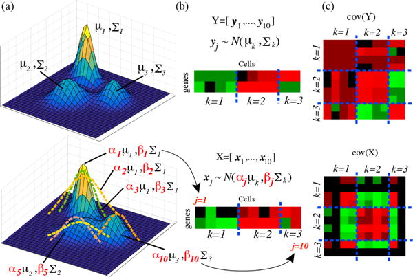
Toy example showing stochastic data generation. Top: Ideal case without technical variation: observations per cell are drawn from a DPMM (a). An example of 10 cells in (b) with block covariance (c). Bottom: When cell-specific variations are present, observations are drawn from a DPMM (a) with scaled cluster-specific moments (b), where block structures can be partially lost (c).

Figure 4.

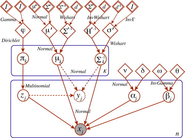
Plate model for BISCUIT. x_j is the observed gene expression of cell j, white circles denote latent variables of interest, rectangles indicate replications with the replicative factor at the bottom right corner, diamonds are hyperparameters and double diamonds are hyperpriors calculated empirically.

A computational challenge in implementing the DPMM is in handling the infinite mixture (Ishwaran & James, 2001) so we use the truncated DP instead (Blei & Jordan, 2004; Ohlssen et al., 2007).

For the Bayesian model setting, we assign conjugate prior distributions to the parameters, namely a symmetric Dirichlet prior of the order K over π, a conjugate-family prior over each μ_k as Normal and for Σ_k as Wishart³, and a Normal for α_j and Inverse-gamma for β_j. We chose non-informative priors over α and β based on empirical observations in library size variation in real datasets (refer Figure 2). An alternative prior construction would be based on the hierarchical Empirical Bayes method (Kucukelbir & Blei). To complete the hierarchical Bayesian specification, we place conjugate hyperpriors over these hyperparameters similar to the conditionally-conjugate model of Görür & Rasmussen (2010).

In the ideal case with no technical variation, we would have observed y_j ∼ N (μ_k, Σ_k) and thus we can use the learned model parameters to correct variations in observed x_js and transform to y_js as explained in Section 6.3.

Entire model specification

$$\begin{array}{c}{\left(\mathbf{x}\right)}_j^{\left(1,\dots ,d\right)}|z_j=k\stackrel{\text{ind}}{~}\mathcal{N}\left({\alpha }_j{\mathbf{\mu }}_k,{\beta }_j{\sum }_k\right)\\ {\mathbf{y}}_j~\mathcal{N}\left({\mathbf{\mu }}_k,{\sum }_k\right)\\ {\mathbf{\mu }}_k~\mathcal{N}\left({\mu }^{\prime },{\sum }^{\prime }\right),{\displaystyle {\sum }_k^{-1}~\mathit{Wish}\left({H^{\prime }}^{-1},{\sigma }^{\prime }\right)}\\ {\mu }^{\prime }~\mathcal{N}\left({\mu }^{″},{\sum }^{″}\right),{{\sum }^{\prime }}^{-1}~\mathit{Wish}\left(d,\frac{1}{d{\sum }^{″}}\right)\\ H^{\prime }~\mathit{Wish}\left(d,\frac{1}{d}{\sum }^{″}\right),{\sigma }^{\prime }~\mathit{inv}\mathit{Gamma}\left(1,\frac{1}{d}\right)-1+d\\ z_j|\mathbf{\pi }\stackrel{\text{iid}}{~}\mathit{Mult}\left(z_j|\mathbf{\pi }\right),\mathbf{\pi }|\phi ,K~\mathit{Dir}\left(\mathbf{\pi }|\frac{\phi }{K},\cdots ,\frac{\phi }{K}\right)\\ {\phi }^{-1}~\mathit{Gamma}\left(1,1\right)\\ {\alpha }_j~\mathcal{N}\left(\nu ,{\delta }^2\right),{\beta }_j~\mathit{InV}\mathit{Gamma}\left(\omega ,\theta \right)\end{array}$$ (1)

where j = (1, ⋯, n), μ″ is the empirical mean and Σ″ is the empirical covariance.

4. Theory

4.1. Model Identifiability

As we intend to learn interpretable and consistent structures (rather than building a solely predictive model), we need to insure model identifiability. Specifically, we need to set constraints on parameters α_j, β_j, μ_k such that the parameter estimates are valid.

Lemma 1

A finite mixture of multivariate Gaussian distributions f(X|m_k, S_k) with means m_k and covariance S_k for component k, is identifiable with permutations in components, i.e. ${\displaystyle {\sum }_{k=1}^K{\pi }_{k}f\left(X|{\mathbf{m}}_k,S_k\right)={\displaystyle {\sum }_{l=1}^{K^{★}}{\pi }_l^{★}f\left(X|{\mathbf{m}}_l^{★},S_l^{★}\right)}}$ implies that K = K^★ and mixtures are equivalent with permutations in components.

Proof is in the Supplementary.

Theorem 2

Defining Θ := {∀j, k : (α_jμ_k, β_jΣ_k)} ∪ {π}, suppose that Θ = Θ^★ and for the prior distributions have $\forall j,k:f\left({\alpha }_j,{\mathbf{\mu }}_k,{\beta }_j,{\sum }_k\right)=f\left({\alpha }_j^{★},{{\mathbf{\mu }}_k}^{★},{\beta }_j^{★},{\sum }_k^{★}\right)$ the following conditions hold, we then have Φ = Φ^★ where Φ := {∀j, k : (α_jμ_k, β_jΣ_k)} ∪ {π}.

$$\forall j:{\mathbf{\mu }}_k\ge {\mathit{\mu }}^{\prime }+\mathit{diag}\left({\sum }^{\prime }\right)\left({\alpha }_j-\nu \right)/\delta ,{\beta }_j\le \frac{\theta }{\omega +1}$$

Proof is presented in the Supplementary. The above theorem provides an identifiability guarantee and specifies conditions needed to be satisfied by the prior. These conditions are considered in the empirical Bayesian approach.

4.2. Weak Posterior Consistency

Let $f_0\left(\mathbf{x}\right):=\mathcal{N}\left(\alpha \mathbf{\mu },\beta \sum \right)\in {\mathrm{ℝ}}^d$ be the true Gaussian density of x with identifiability constraints imposed as in Theorem 2. Let $\mathcal{F}$ be the space of all density functions in ℝ^d w.r.t the Lebesque measure. For a given radius ε, the Kullback-Leibler (KL) neighborhood .

Theorem 3

If f₀(x) is compactly supported and the DP base distribution has support ${\mathrm{R}}^d\times {\mathrm{R}}_{+}^{d\times d}$, then for weak consistency we show that f₀(x) ∈ KL(Π) for every ε > 0.

Proof follows closely to Wu & Ghosal (2010) and is provided in the Supplementary.

5. Inference - Gibbs sampling

Inference is obtained via Gibbs sampling using the Chinese restaurant process (CRP). The conditional posterior distributions for model parameters {π, μ, Σ, α, β, z, μ′, Σ′, H′} based on CRP have analytical forms⁴. The conditional posterior for the latent class assignment variable, z_j is: f(z_j = k|z_−j, φ, μ, Σ) = CRP (z_j|φ)f(x_j|μ, Σ, α, β) which is $\frac{n_k-1}{n-1+\phi }\mathcal{N}\left(x_j|{\alpha }_j{\mathbf{\mu }}_k,{\beta }_j{\sum }_k\right)$ for an existing k and $\frac{\phi /\zeta }{n-1+\phi }\mathcal{N}\left(x_j|{\alpha }_j{\mathbf{\mu }}_{\zeta },{\beta }_j{\sum }_{\zeta }\right)$ for an auxiliary class ζ where μ_ζ and Σ_ζ are sampled from their base distributions; ${\mathbf{\mu }}_{\zeta }~\mathcal{N}\left({\mu }^{\prime },{\sum }^{\prime }\right)$ and ${\displaystyle {\sum }_{\zeta }^{-1}~\mathit{Wish}\left(d,\frac{1}{d{\sum }^{″}}\right)}$ (Görür & Rasmussen, 2010; Neal, 2000).

For the component-specific mean and covariance; μ_k, Σ_k:

$$\begin{array}{l}f\left({\mu }_k|·\right)~\mathcal{N}\left({\mu }_k^p,{\sum }_k^p\right),f\left({\sum }_k^{-1}|·\right)~\mathit{Wish}\left(H,\sigma \right)\\ {\mu }_k^p={\sum }_k^p\left({{\sum }^{\prime }}^{-1}{\mu }^{\prime }+{\sum }_k^{-1}\left({\displaystyle \sum _j{x}_j/{\beta }_j}\right)\right)\\ {\sum }_k^p={\left({{\sum }^{\prime }}^{-1}+{\sum }_k^{-1}{\displaystyle \sum _j{\alpha }_j^2/{\beta }_j}\right)}^{-1}\\ H={\left(H^{\prime }+S_x\right)}^{-1},\sigma ={\sigma }^{\prime }+n_k\end{array}$$ (2)

where n_k is the number of elements in cluster k and S_x = Σ_j((x_j − α_jμ_k)(x_j − α_jμ_k)^T)/β_j). For the cell-specific scaling parameters, α_j and β_j:

$$\begin{array}{l}f\left({\alpha }_j|·\right)~\mathcal{N}\left({\nu }^p,{\delta }^{p^2}\right)\\ {\nu }^p={\delta }^{p^2}\left({\nu }^x/{\delta }^{x^2}\nu /{\delta }^2\right),{\delta }^{p^2}={\left(1/{\delta }^{x^2}+1/{\delta }^2\right)}^{-1}\\ f\left({\beta }_j|·\right)~\mathit{InV}\mathit{Gamma}\left({\omega }^p,{\theta }^p\right),{\omega }^p=\omega +d/2\\ {\theta }^p=\theta +\frac{1}{2}{\left(x_j-{\alpha }_j{\mu }_k\right)}^T{\sum }_k^{-1}\left(x_j-{\alpha }_j{\mu }_k\right)\end{array}$$

where A = (β_jΣ_k)^−1/2, ${\nu }^x={\delta }^{x^2}{\displaystyle {\sum }_q\left\{{\left(A{x}_j\right)}^q{\left(A{\mu }_k\right)}^q\right\}}$, ${\delta }^{x^2}={\left({\displaystyle {\sum }_q{\left(A{\mu }_k\right)}^q}\right)}^{-1}$, and (·)^q denotes the q-th element. For the hyperparameters μ′, Σ′ and H′, the derivations are provided in the Supplementary.

Parallel implementation

We initialize the algorithm as per Equation 1. The Gibbs inference is detailed in Algorithm 1 in the Supplementary. We sample cluster-component parameters μ_k, Σ_k in parallel across ks and sample assignments z_j in parallel across cells. One Gibbs sweep for BISCUIT takes O(n) time. The proof is presented in the Supplementary.

6. Results

6.1. Synthetic Data

Sample Generation

For the simulations, we implemented a data generator that mimics the assumed generative model for X as shown in Figure 3 (bottom panel). Using d = 50 and n = 100, we first construct a Gaussian $X_{50\times 100}^{\mathit{temp}}$ having a K = 3 block covariance. Using this, the hyperparameters, hyperpriors, component parameters and cell-specific scaling parameters are sampled based on Equation 1. Next 100 samples are randomly drawn from $\mathcal{N}\left(\mathbf{\alpha }\mathbf{\mu },\mathbf{\beta }\sum \right)$ and stacked to form X_50×100.

Comparison experiments

We compared the performance of BISCUIT with a number of alternative methods including the naive HDPMM (Görür & Rasmussen, 2010) along with two normalization methods typically used for single-cell data. a) a Generalized Linear Model-based normalization (GLMnorm) where counts are regressed against the library size to get a residual count matrix and b) a Mean-normalized method (MeanNorm) where each cell is scaled by the average library size. Both the residual and mean normalized matrices are log-transformed and used as input to the naive HDPMM. Additionally we compare with non-MCMC methods such as Spectral Clustering (Ng et al., 2002) and Phenograph (PG) (Levine et al., 2015).

We assess the quality of inferred clusters using confusion matrices as described in Supplementary E. The confusion matrices for the different MCMC methods are shown in Figure 5. Figure 6 shows boxplots of F-scores obtained in 15 experiments with randomly generated X for the different methods with pairwise differences in Figure S2. The better performance of BISCUIT is due to its ability to account for cell-specific scalings.

Figure 5.

Left to right: Confusion matrices showing true labels and those from MCMC-based methods.

Figure 6.

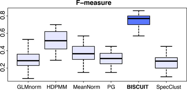
Boxplots of F-scores obtained in 15 experiments with randomly-generated X for various methods.

Model mismatch

In order to test the robustness under model mismatches, we substituted the Gaussian in our data generator with a non-central Student’s t and a negative-binomial to simulate X. These produce a right-skewed fat tail distribution as shown in Figure S3. The negative-binomial distribution is a valid precept used to model single-cell data (Kharchenko et al., 2014). For negative-binomial, the resulting F-scores are in Figure 7 and pairwise comparisons in Figure S5. The F-score plots for Student’s t is given in Figure S6. These figures show BISCUIT is relatively robust under such model mismatches.

Figure 7.

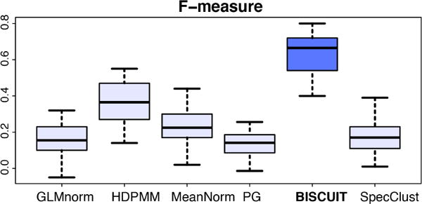
Boxplots of F-scores obtained in 15 experiments with randomly-generated X from a negative binomial distribution.

6.2. Single-cell Gene Expression Data

We evaluated BISCUIT’s performance on real world data using mouse cortex cells from Zeisel et al. (2015) that include ground truth labels for 7 known cell types. For computational speed we chose d = 558 genes with largest standard deviation across n = 3005 cells. Figure S7 shows the confusion matrix for inferred classes and Figure 8 shows the mode of inferred classes across 500 Gibbs sweeps post burn-in of 1500 sweeps compared to their actual cell type labels. Cells are visualized using t-SNE dimensionality reduction (Van der Maaten & Hinton, 2008), as this was shown to be an effective visualization that captures the cell type structure in single-cell data (Amir et al., 2013).

Figure 8.

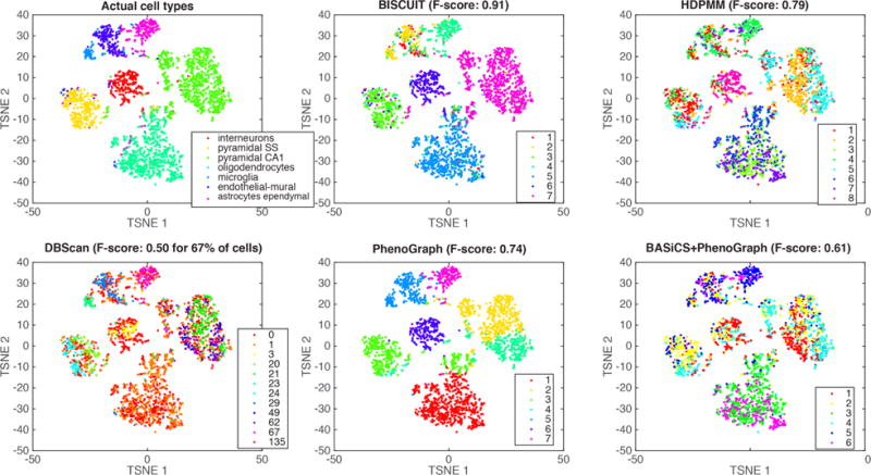
Actual cell types (top left) compared to mode of inferred classes using BISCUIT (top center) versus other comparative approaches for 3005 cells in the (Zeisel et al., 2015) dataset. Cells are projected to 2D using t-SNE (Van der Maaten & Hinton, 2008).

BISCUIT outperforms competing methods including Phenograph (PG), HDPMM, Spectral Clustering (Spec-Clust) and DBscan (Satija et al., 2015) (see Figure 8). We also compared performance to first normalizing with BASiCS (Vallejos & Richardson, 2015) and subsequently clustering using PG, SpecClust, HDPMM and found this to be inferior to clustering without normalization. Refer to Table S1 for F-scores of BISCUIT versus competing methods.

BISCUIT includes two features which improve both the clustering and normalization. First, cells are clustered based on similarity in expression (modeled by cluster means), as well as similar co-expression (covariance) structure between genes. Second, by inferring technical variation parameters (α, β) that normalize cells, we can improve clustering of cells with very different library size but similar co-expressed genes. Figure 9 shows α capturing variation in library size which drives clustering with this normalization. Figure S8 shows the mode of inferred covariances Σ_k for 4 example clusters after performing hierarchical clustering on each matrix, which show distinct patterns of gene co-expressions specific to each cluster. Interpretations and gene annotation enrichment of these structures give insights to gene regulatory relationships and pathways particular to each cell type, which would be followed up in future work.

Figure 9.

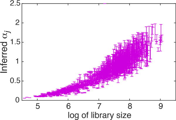
Inferred α_j vs library size per cell j. Errorbars show 1 s.d. across Gibbs sweeps.

6.3. Data Normalization and Imputing

BISCUIT’s key advantage is using a model driven by covariance structures for normalizing and imputing data. For a realistic evaluation, we simulated dropouts from a real world dataset. The Zeisel et al. (2015) dataset was ideal due to its deep coverage (2 million reads per cell compared to the typical 10K-200K reads per cell). To minimize the degree of dropouts and library size variation in the original dataset, we selected a narrow window of m = 500 cells (Figure 1) from the tail of high coverage cells. Then to simulate dropouts, we down-sample counts for each cell j with a different rate r_j ∼ Unif(0.1, 1) to generate a set of observations X = {x₁, …, x_m}, with known down-sampling (DS) rates. The DS is specifically done on the counts (prior to taking log) to simulate library size variation.

Figure 10 shows we successfully infer the normalization parameter α to positively correlate with the degree of DS rates. Also, in lower DS rates with most of the data discarded, simulated data is noisier and intuitively, larger values are inferred for β to scale and correct the variance. We also evaluated the performance in inferring clusters in this more challenging dataset. Figure 11 shows good performance in clustering. To further explore the performance versus percentage of data lost, we estimated F-measures using a sliding window with length 0.05 and overlaps of 0.01 on DS rates. We averaged the performance across all Gibbs samples. Repeating this experiment on 10 different down-sampled datasets, the average performance is depicted in Figure 11, showing almost no impact when > 50% of counts are retained and decent performance in typical scenarios where 70 – 90% of transcripts are lost.

Figure 10.

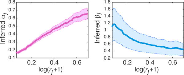
Inferred α_j, β_j vs log of down-sampling rates r_j per cell; shaded areas show 70% confidence intervals.

Figure 11.

Mode of inferred classes for an imputed dataset generated by down-sampling (DS) 500 cells from a real dataset (middle), compared to actual cell types (left). F-measure vs center of a sliding window on DS rates (r) for 10 different down-sampled datasets got with different rates, averaged across Gibbs sweeps; shaded area shows 70% confidence interval.

To evaluate the performance of imputing dropouts and normalization, we use the inferred model parameters to impute corrected data. Specifically, we transform simulated data ${\mathbf{x}}_j~\mathcal{N}\left({\alpha }_j{\mathbf{\mu }}_k,{\beta }_j{\sum }_k\right)$ to imputed data ${\mathbf{y}}_j~\mathcal{N}\left({\mathbf{\mu }}_k,{\sum }_k\right)$. Assuming a linear transformation y_j = Ax_j + b, we have μ_k = αAμ_k + b and Σ_k = βAΣ_kA^T. Solving these equations for A and b, we have $A=V{\Lambda }^{1/2}{\sum }_k^{-1/2}$ and b = (I − αA)μ_k given the SVD decomposition $\frac{1}{\beta }{\sum }_k=V\Lambda V^T$. Using this transformation, we estimated imputed values y_js from down-sampled x_js, given the inferred parameters μ_k, Σ_k, z, α, β. Figure 12 shows the density plot for imputed values vs original y_j values. We compared the performance in recovering values to the common approach of normalization by library size (Macosko et al., 2015; Brennecke et al., 2013; Buettner et al., 2015). In this approach, the values of each cell x_j are divided by library size and multiplied by mean library size across cells. Figure 12 shows the superiority of our method in recovering dropouts. Counts which are down-sampled to zero cannot be recovered with normalization (abundance of zero values in normalized X on right panel), while our method can successfully recover them (left panel). The proportion of dropouts in this down-sampled dataset was 21% and due to their overlaps at zero, they are not emphasized. Addressing this problem is very crucial in real datasets which could contain up to 50% dropouts.

Figure 12.

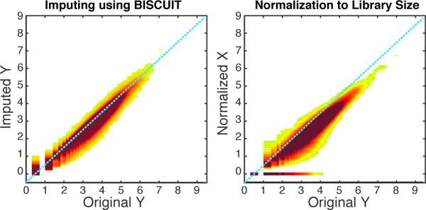
Density plot of imputed values with BISCUIT (left) and normalization to library size (right) on a down-sampled dataset vs original values prior to down-sampling.

7. Conclusion

Single-cell RNA-seq produces vast amounts of noisy, heterogeneous sparse data and therefore requires development of appropriate computational techniques. In this paper, we address a number of these problems and present our model, BISCUIT, that concurrently clusters cells and learns co-expression structures specific to each cluster while inferring parameters capturing technical variation (e.g. library size variation). Using these inferred parameters, we are able to normalize single-cell data and impute dropouts. We show accurate clustering on known cell types and improvement over previous approaches. In future work, we will apply BISCUIT to understand tumor heterogeneity and other primary tissue to characterize and interpret novel cell types. This method could also be extended to other application domains where variation among clusters exhibit heteroscedasticity.

References

- Amir El-ad David, Davis Kara L, Tadmor Michelle D, Simonds Erin F, Levine Jacob H, Bendall Sean C, Shenfeld Daniel K, Krishnaswamy Smita, Nolan Garry P, Pe’er Dana. visne enables visualization of high dimensional single-cell data and reveals phenotypic heterogeneity of leukemia. Nature biotechnology. 2013;31(6):545–552. doi: 10.1038/nbt.2594. [DOI] [PMC free article] [PubMed] [Google Scholar]
- Anders Simon, Huber Wolfgang. Differential expression analysis for sequence count data. 2010 doi: 10.1186/gb-2010-11-10-r106. [DOI] [PMC free article] [PubMed] [Google Scholar]
- Antoniak Charles E. Mixtures of dirichlet processes with applications to bayesian nonparametric problems. The Annals of Statistics. 1974:1152–1174. [Google Scholar]
- Bengio Yoshua. Statistical language and speech processing. Springer; 2013. Deep learning of representations: Looking forward. In; pp. 1–37. [Google Scholar]
- Blei David M, Jordan Michael I. Variational methods for the dirichlet process. In: Brodley Carla E., editor. Proceedings of the International Conference on Machine Learning (ICML 2004) Vol. 69. 2004. (ACM International Conference Proceeding Series). [Google Scholar]
- Brennecke Philip, Anders Simon, Kim Jong Kyoung, Kołodziejczyk Aleksandra A, Zhang Xiuwei, Proserpio Valentina, Baying Bianka, Benes Vladimir, Teichmann Sarah A, Marioni John C, et al. Accounting for technical noise in single-cell rna-seq experiments. Nature methods. 2013;10(11):1093–1095. doi: 10.1038/nmeth.2645. [DOI] [PubMed] [Google Scholar]
- Buettner Florian, Natarajan Kedar N, Casale F Paolo, Proserpio Valentina, Scialdone Antonio, Theis Fabian J, Teichmann Sarah A, Marioni John C, Stegle Oliver. Computational analysis of cell-to-cell heterogeneity in single-cell rna-sequencing data reveals hidden subpopulations of cells. Nature biotechnology. 2015;33(2):155–160. doi: 10.1038/nbt.3102. [DOI] [PubMed] [Google Scholar]
- Di Palma Serena, Bodenmiller Bernd. Unraveling cell populations in tumors by single-cell mass cytometry. Current opinion in biotechnology. 2015;31:122–129. doi: 10.1016/j.copbio.2014.07.004. [DOI] [PubMed] [Google Scholar]
- Dıaz-Garcıa José A, Jáimez Ramón Gutierrez, Mardia Kanti V. Wishart and pseudo-wishart distributions and some applications to shape theory. Journal of Multivariate Analysis. 1997;63(1):73–87. [Google Scholar]
- Fan Jean, Salathia Neeraj, Liu Rui, Kaeser Gwendolyn E, Yung Yun C, Herman Joseph L, Kaper Fiona, Fan Jian-Bing, Zhang Kun, Chun Jerold, et al. Characterizing transcriptional heterogeneity through pathway and gene set overdispersion analysis. Nature Methods. 2016 doi: 10.1038/nmeth.3734. [DOI] [PMC free article] [PubMed] [Google Scholar]
- Gawad Charles, Koh Winston, Quake Stephen R. Dissecting the clonal origins of childhood acute lymphoblastic leukemia by single-cell genomics. Proceedings of the National Academy of Sciences. 2014;111(50):17947–17952. doi: 10.1073/pnas.1420822111. [DOI] [PMC free article] [PubMed] [Google Scholar]
- Görür Dilan, Rasmussen Carl Edward. Dirichlet process gaussian mixture models: Choice of the base distribution. In. Journal of Computer Science and Technology. 2010:653–664. [Google Scholar]
- Hashimshony Tamar, Wagner Florian, Sher Noa, Yanai Itai. Cel-seq: single-cell rna-seq by multiplexed linear amplification. Cell reports. 2012;2(3):666–673. doi: 10.1016/j.celrep.2012.08.003. [DOI] [PubMed] [Google Scholar]
- Hollander Myles, Wolfe Douglas A. Nonparametric Statistical Methods Wiley Interscience. (2nd) 1999 [Google Scholar]
- Ishwaran Hemant, James Lancelot F. Gibbs sampling methods for stick-breaking priors. In. Journal of the American Statistical Association. 2001:161–173. [Google Scholar]
- Jaitin Diego Adhemar, Kenigsberg Ephraim, Keren-Shaul Hadas, Elefant Naama, Paul Franziska, Zaretsky Irina, Mildner Alexander, Cohen Nadav, Jung Steffen, Tanay Amos, et al. Massively parallel single-cell rna-seq for marker-free decomposition of tissues into cell types. Science. 2014;343(6172):776–779. doi: 10.1126/science.1247651. [DOI] [PMC free article] [PubMed] [Google Scholar]
- Junker Jan Philipp, van Oudenaarden Alexander. Every cell is special: genome-wide studies add a new dimension to single-cell biology. Cell. 2014;157(1):8–11. doi: 10.1016/j.cell.2014.02.010. [DOI] [PubMed] [Google Scholar]
- Kharchenko Peter V, Silberstein Lev, Scadden David T. Bayesian approach to single-cell differential expression analysis. Nature methods. 2014;11(7):740–742. doi: 10.1038/nmeth.2967. [DOI] [PMC free article] [PubMed] [Google Scholar]
- Klein Allon M, Mazutis Linas, Akartuna Ilke, Tallapragada Naren, Veres Adrian, Li Victor, Peshkin Leonid, Weitz David A, Kirschner Marc W. Droplet barcoding for single-cell transcriptomics applied to embryonic stem cells. Cell. 2015;161(5):1187–1201. doi: 10.1016/j.cell.2015.04.044. [DOI] [PMC free article] [PubMed] [Google Scholar]
- Korwar Ramesh M, Hollander Myles. Contributions to the theory of dirichlet processes. The Annals of Probability. 1973:705–711. [Google Scholar]
- Kucukelbir Alp, Blei David M. Population empirical bayes [Google Scholar]
- Lamoureux Christopher G, Lastrapes William D. Heteroskedasticity in stock return data: volume versus garch effects. The Journal of Finance. 1990;45(1):221–229. [Google Scholar]
- Levine Jacob H, Simonds Erin F, Bendall Sean C, Davis Kara L, Elad D Amir, Tadmor Michelle D, Litvin Oren, Fienberg Harris G, Jager Astraea, Zunder Eli R, et al. Data-driven phenotypic dissection of aml reveals progenitor-like cells that correlate with prognosis. Cell. 2015;162(1):184–197. doi: 10.1016/j.cell.2015.05.047. [DOI] [PMC free article] [PubMed] [Google Scholar]
- Lilliefors Hubert W. On the kolmogorov-smirnov test for normality with mean and variance unknown. Journal of the American Statistical Association. 1967;62(318):399–402. [Google Scholar]
- Macosko Evan Z, Basu Anindita, Satija Rahul, Nemesh James, Shekhar Karthik, Goldman Melissa, Tirosh Itay, Bialas Allison R, Kamitaki Nolan, Martersteck Emily M, et al. Highly parallel genome-wide expression profiling of individual cells using nanoliter droplets. Cell. 2015;161(5):1202–1214. doi: 10.1016/j.cell.2015.05.002. [DOI] [PMC free article] [PubMed] [Google Scholar]
- Navin Nicholas E. Cancer genomics: one cell at a time. Genome Biol. 2014;15:452. doi: 10.1186/s13059-014-0452-9. [DOI] [PMC free article] [PubMed] [Google Scholar]
- Neal Radford M. Markov chain sampling methods for dirichlet process mixture models. Journal of computational and graphical statistics. 2000;9(2):249–265. [Google Scholar]
- Ng Andrew Y, et al. On spectral clustering: Analysis and an algorithm. 2002 [Google Scholar]
- Ohlssen David I, Sharples Linda D, Spiegelhalter David J. Flexible random-effects models using bayesian semi-parametric models: applications to institutional comparisons. (ACM International Conference Proceeding Series).Statistics in Medicine. 2007;26(9):2088–2112. doi: 10.1002/sim.2666. [DOI] [PubMed] [Google Scholar]
- Oshlack Alicia, Robinson Mark D, Young Matthew D, et al. From rna-seq reads to differential expression results. Genome biol. 2010;11(12):220. doi: 10.1186/gb-2010-11-12-220. [DOI] [PMC free article] [PubMed] [Google Scholar]
- Paul Franziska, Arkin Yaara, Giladi Amir, Jaitin Diego Adhemar, Kenigsberg Ephraim, Keren-Shaul Hadas, Winter Deborah, Lara-Astiaso David, Gury Meital, Weiner Assaf, et al. Transcriptional heterogeneity and lineage commitment in myeloid progenitors. Cell. 2015;163(7):1663–1677. doi: 10.1016/j.cell.2015.11.013. [DOI] [PubMed] [Google Scholar]
- Rasmussen Carl Edward. The infinite gaussian mixture model. 1999 [Google Scholar]
- Satija Rahul, Farrell Jeffrey A, Gennert David, Schier Alexander F, Regev Aviv. Spatial reconstruction of single-cell gene expression data. Nature biotechnology. 2015;33(5):495–502. doi: 10.1038/nbt.3192. [DOI] [PMC free article] [PubMed] [Google Scholar]
- Schwartz Lorraine. On bayes procedures. Zeitschrift fr Wahrscheinlichkeitstheorie und Verwandte Gebiete. 1965;4(1):10–26. doi: 10.1007/BF00535479. [DOI] [Google Scholar]
- Shalek Alex K, Satija Rahul, Adiconis Xian, Gertner Rona S, Gaublomme Jellert T, Raychowdhury Raktima, Schwartz Schraga, Yosef Nir, Malboeuf Christine, Lu Diana, et al. Single-cell transcriptomics reveals bimodality in expression and splicing in immune cells. Nature. 2013;498(7453):236–240. doi: 10.1038/nature12172. [DOI] [PMC free article] [PubMed] [Google Scholar]
- Stegle Oliver. Computational and analytical challenges in single-cell transcriptomics. Nature Publishing Group; Jan, 2014. pp. 133–145. [DOI] [PubMed] [Google Scholar]
- Titterington DM. Common structure of smoothing techniques in statistics. International Statistical Review/Revue Internationale de Statistique. 1985:141–170. [Google Scholar]
- Vallejos Catalina A, Marioni John C, Richardson Sylvia. Basics: Bayesian analysis of single-cell sequencing data. PLoS Computational Biology. 2015;11(6):e1004333. doi: 10.1371/journal.pcbi.1004333. [DOI] [PMC free article] [PubMed] [Google Scholar]
- Van der Maaten Laurens, Hinton Geoffrey. Visualizing data using t-sne. Journal of Machine Learning Research. 2008;9(2579-2605):85. [Google Scholar]
- Wu Yuefeng, Ghosal Subhashis. The l1-consistency of dirichlet mixtures in multivariate bayesian density estimation. Journal of Multivariate Analysis. 2010;101(10):2411–2419. [Google Scholar]
- Yakowitz Sidney J, Spragins John D. On the identifiability of finite mixtures. The Annals of Mathematical Statistics. 1968:209–214. [Google Scholar]
- Zeisel Amit, Muñoz-Manchado Ana B, Codeluppi Simone, Lönnerberg Peter, La Manno Gioele, Juréus Anna, Marques Sueli, Munguba Hermany, He Liqun, Betsholtz Christer, et al. Cell types in the mouse cortex and hippocampus revealed by single-cell rna-seq. Science. 2015;347(6226):1138–1142. doi: 10.1126/science.aaa1934. [DOI] [PubMed] [Google Scholar]
Associated Data
This section collects any data citations, data availability statements, or supplementary materials included in this article.