Homogeneous Time Constants Promote Oscillations in Negative Feedback Loops

Abstract

Biological oscillators are present in nearly all self-regulating systems, from individual cells to entire organisms. In any oscillator structure, a negative feedback loop is necessary, but not sufficient to guarantee the emergence of periodic behaviors. The likelihood of oscillations can be improved by careful tuning of the system time constants and by increasing the loop gain, yet it is unclear whether there is any general relationship between optimal time constants and loop gain. This issue is particularly relevant in genetic oscillators resulting from a chain of different subsequent biochemical events, each with distinct (and uncertain) kinetics. Using two families of genetic oscillators as model examples, we show that the loop gain required for oscillations is minimum when all elements in the loop have the same time constant. On the contrary, we show that homeostasis is ensured if a single element is considerably slower than the others.

Timekeeping elements coordinate and synchronize most processes required to sustain life, from the physiology of individual cells to the daily rhythms of entire organisms.¹ The design principles underlying the operation of biomolecular clocks have been investigated by dissecting natural systems,²⁻⁵ as well as by building de novo molecular oscillators in an effort to identify minimal requirements for periodic behaviors.⁶⁻¹⁰ Experiments^6,2,7,9,11 and modeling¹²⁻²¹ have established that a necessary requirement for a system to exhibit oscillations is the presence of a negative loop. Conversely, any negative feedback loop potentially leads to oscillations provided that the loop includes destabilizing features, for instance delaying elements associated with a large feedback gain.^7,22,23 Delay can be introduced by a variety of phenomena. In addition to transcription and translation steps, delay is increased by transport, mRNA splicing and stabilization, phosphorylation, and protein maturation.^24,25,43 While an explicit delay term is useful to aggregate these phenomena in a single, black-box parameter, in other instances it is possible to model their individual kinetics as a chain of interconnected subsystems.^17,25,26 In a linearized closed-loop system, a chain of slow subsystems has the same effects as an explicit delay in inducing oscillations.²² The overall delay of the negative feedback chain depends on all the time constants of the dynamic elements. Given a sufficient delay, the larger the feedback gain, the likelier is the onset of persistent oscillations.

Despite the simplicity of these design principles, it is unclear how the individual time constants and the overall gain affect the emergence of oscillations. Are we equally likely to observe oscillations in a system with homogeneous versus nonhomogeneous time scales? How large should the loop gain be in either case? These questions are particularly relevant in the context of genetic oscillators, where time constants are determined by mRNA and protein degradation, transport, and processing rates, which may widely vary among the oscillator components, and a large loop gain is energetically expensive, because it depends on the production rate of the components.

In this paper, we address the following question in mathematical terms: Given a negative loop of first order elements, each associated with its own time constant, which is the choice of the time constants that requires the smallest gain to allow for persistent oscillations? We demonstrate that homogeneous time constants are the most favorable choice when a small loop gain is desired. In particular we prove that (1) the smallest negative feedback gain required to trigger oscillations is achieved when all time constant are equal; (2) the smallest gain is invariant under a homogeneous scaling of all time constants and the period of the oscillations is proportional to the scaling factor; (3) as a converse result, in a negative feedback loop, the best strategy to avoid oscillations is to have a single element of the chain that is much slower than all the others, and this fact explains why, in several pathways with negative feedback, the presence of a slow element ensures a robust nonoscillatory behavior.

We apply our results to well-known genetic oscillators, the Goodwin oscillator and a two-node (inhibitor-activator) oscillator, and we derive exact (necessary and sufficient) conditions for the existence of parameters that ensure oscillations.

Architecture of Candidate Negative Feedback Oscillators

As candidate oscillator architectures, we consider negative feedback loops of the following form:

1

representing the series connections of n ordered subsystems in which any element has a positive influence, quantified by parameters b_i > 0 (with i = 2, ..., n), on the next one, while u is a perturbing input that triggers oscillations. Each ordinary differential equation (ODE) in the model in eq 1 is suited to model phenomena such as production, conversion, processing, and degradation of molecular components (mRNA and proteins) interconnected in a regulatory chain.²⁷ The model can also capture enzymatic processes that operate at low substrate concentration relative to the binding affinity of the enzyme and substrate; in this regime, Michaelian or Hill-type reaction rates become approximately linear (first-order rates). A negative feedback loop is generated via the inhibitory effect of the last element in the chain on the first one, quantified by parameter b₁ > 0. The parameter τ_i represents the time constant of process i (which can be seen as the speed of the reaction of the species x_i due to the regulatory effect of x_i–1).

A similar negative feedback structure can be found in many oscillatory systems.¹⁷ We now take the Laplace transform of these ODEs: we formally replace x_i(t) with X_i(s) and the derivative d/dt with the complex variable s, ẋ_i(t) → sX_i(s). After Laplace-transformation, the model in eq 1 can be rewritten as a block-interconnection of elements:

as shown in Figure 1.

Figure 1.

Loop of n first order systems: block diagram.

The quantity

is called the loop gain and has a fundamental role. It is the product of all the interaction strengths and thus represents the cumulative strength of the loop. It turns out that the characteristic polynomial depends on the product κ only, and not on the individual parameters b_i; hence, even if the individual rates b_i are changed, the system behavior remains the same as long as their product is unchanged (see the Supporting Information for the detailed derivation). The onset of oscillations in this negative feedback loop is therefore associated with two fundamental ingredients:

• The time constants τ_i, which introduce an overall delay in the loop;

• A sufficiently large feedback gain κ > 0.

In the next section we ask ourselves whether there is any ideal relationship between the loop gain and the time constants to achieve or avoid oscillatory behavior.

Influence of Time Constants on the Oscillatory Regime

We next investigate how the time constants τ_i influence the onset of persistent oscillations. We define τ = [τ₁ τ₂ ... τ_n], the vector of time constants, and consider the characteristic polynomial associated with the (linearized) system of ODEs:

2

For κ = 0, the roots of p_n(s, τ) are λ_i = −1/τ_i, real and negative, hence the system response has an exponentially decreasing pattern. For large values of κ, p_n(s, τ) has complex roots, associated with oscillations.

The oscillations are damped if the roots have a negative real part. To have persistent oscillations, the roots of p_n(s, τ) must reach and cross the imaginary axis in the complex plane. This can happen only if

(as discussed at the end of this section; see also ref (28)). Henceforth, we assume that the necessary condition n ≥ 3 is verified.

For n ≥ 3, let us increase κ. Then, there exists a critical gain κ* such that, for all κ > κ*, p_n(s, τ) has complex roots with positive real part (namely, the system becomes unstable). For κ = κ*, p_n(s, τ) has two purely imaginary roots ± jω*, while the other roots have negative real part. The limit value κ* is associated with the onset of an oscillation with frequency ω*/2π; we call ω* critical pulsation. Note that ω* ≠ 0: p_n(s, τ) cannot have 0 as a root for κ > 0, since p(0, τ) = κ + 1 ≠ 0.

We can formally define the critical gain κ* as the smallest value of κ for which p_n(s, τ) has a pair of purely imaginary roots (corresponding to the stability limit). The value κ* depends on the time constants τ_i and we can write

3

Which are the most favorable values of τ_i to promote oscillations? We address this question in terms of the minimum critical gain, by seeking a value τ* = [τ₁^* τ₂ ... τ_n^*] that minimizes the critical κ*(τ) enabling the onset of oscillations.

Problem: Find a value τ* that minimizes κ*(τ) in eq 3.

Main result: The problem is solved by a value τ* with

This result is proved in the Supporting Information (Theorem 1): our proofs are based on frequency analysis tools, linear algebraic tools and principles of convex optimization.

Therefore, an essential factor to promote oscillations in a negative feedback loop is the homogeneity of the time constants of the subsystems involved in the loop.

Further, we find that scaling the time constants influences exclusively the critical pulsation, without affecting the critical gain: when the time constants are scaled as τ_i → στ_i, for arbitrary σ > 0, the critical gain κ* is invariant, κ*(στ*) = κ*(τ*), while the critical pulsation scales proportionally to σ: ω* → σω* (cf. Corollary 1, Supporting Information).

Also, the critical gain κ* is a decreasing function of the number of elements in the loop (see the Supporting Information, Proposition 2, for details).

Our result (the critical gain that allows for oscillations is minimized when all the time constants are equal) indirectly suggests how to prevent a system from oscillating. This aspect is relevant in the context of biological and biochemical feedback loops, in all the situations where it is important to preserve homeostasis and oscillatory behaviors must be avoided. Being κ* a decreasing function of n, long feedback chains are more prone to instability, which can be of an oscillatory type. Hence, a natural question is which is the best strategy to avoid oscillations in the loop. Our result suggests that incongruous time constants lead to a robustly nonoscillatory behavior. Let us now consider the complementary question: assuming (without restriction) that the time constants are normalized as

where T_tot is the overall loop delay, which is the best distribution of time constants to prevent oscillatory behaviors? We find that, roughly speaking, it is better to have the delay concentrated in a single subsystem (see the Supporting Information, Proposition 3, for details). Then, a robust strategy to prevent oscillations is, for instance, including in the loop a single subsystem that is much slower than the others, so that their time constant is negligible with respect to the slow part. This result also explains the previous statement about the necessity of condition n ≥ 3 to have persistent oscillations. Indeed, setting τ_i = 0 is mathematically equivalent to neglecting the ith process, since then 1/(1 + τ_is) = 1.

A fundamental consequence of our results is the following: in a negative feedback loop, the presence of a single slow element is an effective strategy to preserve stability and prevent oscillations. Indeed, several negative feedback loops in nature are practically always stable, and this can be explained by noting that the involved time constants are very different. For example, biologically, degradation rates of mRNA and proteins may vary in a broad range and, as foreseen by our results, this variability could contribute to stabilizing negative loops, making it difficult to achieve oscillations. Yet, we point out that, when the kinetics of a molecular species are much slower or much faster than the rest of the system, they can be simply eliminated from the model via time scale separation methods;²⁷ this type of drastic time scale variability may affect the capacity for oscillations when the system dimension collapses below 3.

Examples

Our results allow us to derive analytical bounds in the parameter space for the oscillatory regions of general families of genetic oscillators. These bounds are also numerically verified in the following sections via random parameter sampling.²⁹

Goodwin Oscillator

The well-known Goodwin oscillator³⁰ is associated with the following equations:

4

5

The model is characterized by the number n of stages, by the cooperativity (Hill) coefficient N, by the apparent dissociation constant K, and by the rate constants a_i and b_i. Rates a_i and b_i can model protein translation and degradation, mRNA processing phenomena, or protein phosphorylation/dephosphorylation.³¹ All these parameters are positive. As shown in the Supporting Information (Section 2.1), the system admits a single positive equilibrium. The emergence of sustained oscillations depends on the choice of the parameters, which influences the values of both the variables at steady-state and of the entries of the Jacobian matrix. By applying our main result to the Goodwin oscillator model, we discover that there exists at least one choice of the parameter values that leads to oscillations (namely, for which the linearized system admits complex eigenvalues with nonnegative real part) if and only if

6

(the full derivation is in the Supporting Information, Section 2.3). The characteristic equation, equating the characteristic polynomial to zero, is

7

Here, x̅_n is the steady state value of x_n derived by solving the equilibrium equation

8

from which existence and uniqueness of the equilibrium are proven in the Supporting Information (Section 3.1). If we could arbitrarily choose the rates a_i and b_i, then we could achieve any positive steady-state x̅_n. Hence, the gain in eq 7,

could take any value in the interval: 0 < κ(x̅_n) < N. The value of the ith time constant for this system is τ_i = 1/b_i. Hence, our result tells us that the (minimum) critical gain is obtained by setting b₁ = b₂ = ... = b_n = b (which leads to equal time constants), hence

9

The condition in eq 6 is necessary and sufficient for eq 9 to admit imaginary solutions. As exemplified in Figure 2, if the condition in eq 6 is satisfied, oscillations are possible if the rates a_i are large enough with respect to the rates b_i; this guarantees a large equilibrium value x̅_n, hence κ(x̅_n) is larger than the critical gain.

Figure 2.

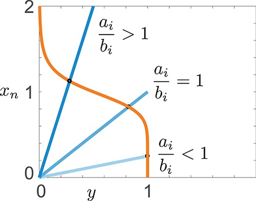
Goodwin oscillator: equilibrium conditions for different ratios a_i/b_i. The orange line represents the first expression in eq 8, while the blue lines represent the second expression in eq 8 for different values of the ratios a_i/b_i. Their intersections give, on the vertical axis, the equilibrium values of x_n for various choices of a_i/b_i.

Note that, if the oscillator includes three stages (n = 3), the condition in eq 6 becomes and the minimum value of the Hill coefficient N to have oscillations is N = 8, consistently with the results in ref (32).

In Figure 3 we numerically compute the oscillatory region in the N–n space when a_i = a and b_i = b, for all i. In each panel, the black line represents the condition in eq 6 converted to an equality, and delimits the region where oscillations can occur. As a further numerical experiment, we fixed a_i = a for all i and randomly generated different values of the parameters b_i, taken from different distributions (normal and uniform distribution) with the same expected value E[b_i] = 1 and variance ϵ. With this sampling method, the total delay is not necessarily constant for all samples: the degradation rates are randomly generated and are drawn from different distributions, which all have the same average, but which can be more or less spread depending on the value of the variance ϵ. The lower the variance, the more homogeneous are the degradation rates b_i. Figure 4 shows the fraction of oscillating samples (parameter choices for which characteristic polynomial has positive-real-part roots) as a function of ϵ. As predicted by our analytical results, decreasing the variance increases the likelihood of oscillations. Choosing homogeneous time constants favors oscillations, but also other design decisions are important: for instance, the overall loop gain needs to be high enough.

Figure 3.

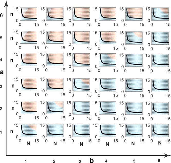
Oscillatory domain of the Goodwin oscillator with K = 1 in the (n, N) plane, for various choices of homogeneous rates, a_i = a and b_i = b for all i. The black line represents ; hence, eq 6 is satisfied in the whole region above. We compute the solutions of eq 9: red dots indicate an oscillatory behavior, blue dots indicate no oscillations, while gray dots indicate that no equilibrium can be found computationally due to numerical problems.

Figure 4.

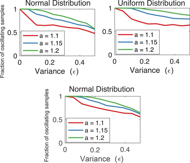
The fraction of oscillating samples of the Goodwin oscillator is largest when randomly drawn degradation rates are homogeneous. We simulated the model with K = 1 and n = 5; in the top panels N = 8, while in the bottom panel N = 10. We took a_i = a and randomly generated rates b_i with expected value E[b_i] = 1 and variance ϵ. (In each simulation, the randomly generated parameters are kept constant during all the integration steps of the ODEs.) We show the fraction of oscillating samples as a function of the variance ϵ when the rates b_i are taken from a normal distribution (top left, and bottom) and a uniform distribution (top right). In all panels, 1000 parameter samples are drawn per data point.

A Two-Node Oscillator

Consider a two-node oscillator given by the feedback interconnection of an activated module and an inhibited module:^9,48−50

10

11

12

13

The ODEs of variables r₁ and r₂ represent mRNA dynamics, and p₁, p₂ represent protein translation. As earlier, N is a Hill coefficient, and K₁ and K₂ are apparent dissociation constants. Parameters α₁ and α₂ are maximal mRNA transcription rates, and β₁, β₂ are mRNA degradation rates. Finally γ₁, γ₂ and δ₁, δ₂ are protein translation and degradation rates. This model can serve as a coarse-grained representation of a variety of molecular clocks. Many genetic oscillators result from the interconnected dynamics of inhibitor-activator elements,²⁵ such as the p53-mdm-2³³ and the IκB-NF-κB³⁴ oscillators; this architecture has also been demonstrated in artificial in vitro transcriptional oscillators.^9,35,36 Here we assume that the mRNA dynamics evolve on a time scale that is comparable to that of the proteins; this means that the order of the model cannot be reduced via time scale separation arguments. On the basis of our main result, we can prove that there exists at least one choice of parameters for which the system exhibits sustained oscillations (namely, the linearized system has complex eigenvalues with a nonnegative real part) if and only if

14

The linearized system has characteristic equation

15

where p̅₁ and p̅₂ are the steady-state values of p₁ and p₂. The loop gain

ranges in the interval 0 < κ(p̅₁, p̅₂) < N²; it is a decreasing function of p̅₁, and an increasing function of p̅₂. In view of our main result, the minimum critical gain guaranteeing oscillations is achieved when β₁ = β₂ = δ₁ = δ₂ = τ. The corresponding critical equation is

therefore no unstable complex eigenvalues, hence no oscillations, can be found unless N > 2 (the full derivation is in the Supporting Information, Section 3.3). Numerical simulations illustrating and confirming this analytical result are in Figure 5. We have also generated random instances of the oscillator to show how increasing the variance in the delay decreases the chances of oscillatory behavior (Figure 6). We note that in this particular example, if the mRNA dynamics are much faster than the protein dynamics, the model can be reduced to include exclusively the protein kinetics; in that case, oscillations cannot be achieved for any choice of the parameters.

Figure 5.

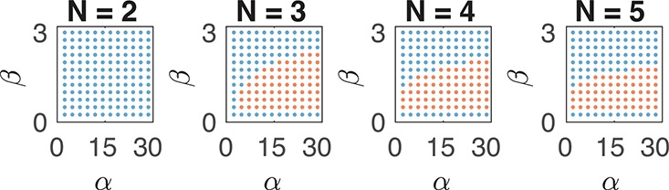
Oscillatory regime of the two-node oscillator. We compute the solutions of eq 15, with α₁ = α₂ = α, β₁ = β₂ = β, γ₁ = γ₂ = 1, δ₁ = δ₂ = 1 and K₁ = K₂ = 1, and indicate with red dots an oscillatory behavior, with blue dots no oscillations. Parameter sets that give rise to oscillations cannot be found for N = 2, while they are easy to find for N > 2.

Figure 6.

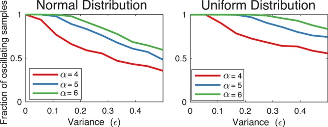
The fraction of oscillating samples of the two-node oscillator is largest when randomly drawn degradation rates are homogeneous. We simulated the model with N = 3, γ₁ = γ₂ = 1, K₁ = K₂ = 1, α₁ = α₂ = α and randomly generated (β_i, δ_i) with expected value E[(β_i, δ_i)] = (1, 1) and variance ϵ. (In each simulation, the randomly generated parameters are kept constant during all the integration steps of the ODEs.) We show the fraction of oscillating samples as a function of the variance ϵ when (β_i, δ_i) are taken from a normal distribution (left) and a uniform distribution (right). 1000 parameter samples are drawn per data point.

Conclusion and Discussion

We have demonstrated that homogeneity of the time constants within a negative feedback loop can facilitate the emergence of oscillations, in that it minimizes the critical loop gain (minimum gain to achieve oscillations). We have also shown that scaling of the (uniform) time constants influences the critical frequency, but does not affect the critical gain. A converse result is that a candidate oscillator can be stabilized, i.e., oscillations cannot occur, by increasing a single (arbitrarily chosen) time constant of the loop with respect to the others. The negative feedback architecture we consider is general, and it can be specialized to model many biomolecular oscillators.²⁵

The gain of the biomolecular feedback loops we consider is proportional to the ratio of production and degradation rates of its components, and to the cooperativity coefficient of regulatory molecules (Hill coefficient N). Maintaining the lowest gain that can yield oscillations in the network is therefore tantamount to operating the circuit with minimum consumption of transcription and translation resources, minimum kinase activity, as well as with minimum copy number of regulators. This energy-efficient scenario can be achieved when the time constants in each process are similar (degradation, transport, and processing rates). This requirement may be easy to satisfy if these time constants are globally regulated for all components (for instance, mRNA and protein degradation).

It must be pointed out that, in our analysis, we have considered systems consisting of a single negative feedback loop: although this is a very common structure for biological oscillators,^17,25 it is not the only one. For this particular structure, we have argued that

• Short negative loops have a stabilizing effect (which makes the onset of sustained oscillations less likely, because a higher loop gain is needed);

• Long negative loops can favor the onset of sustained oscillations, and the most favorable case is that in which the time constants of the system in the loop are similar;

• If one or two time constants are significantly larger than the others, then the long loop actually behaves as a short one and the probability of having sustained oscillations is smaller (because a higher loop gain is needed for the onset of oscillations).

However, if several feedback loops are concurrently present, our analysis does not apply, and the above statements are no longer true. In particular, our findings are valid in the absence of self-catalytic reactions (i.e., of positive self-loops). In the presence of a positive self-loop, also a single negative loop involving two nodes only can be easily destabilized. For instance, consider the system

where a, b, c and d are positive parameters. As shown by our results, this loop cannot be destabilized. However, this system can exhibit sustained oscillations if a can be negative (take for instance a = −d): in this case our results no longer hold, because now x₁ is self-catalytic.

In practice, positive self-loops are not very common. Yet, a positive feedback loop can result from a chain of reactions. Indeed, different oscillator architectures are based on the coexistence of positive and negative loops (it is important to stress that the presence of a negative loop is necessary for the onset of oscillations^14,15). In particular

• A (possibly short) negative loop can be destabilized by the concurrent presence of another loop that is positive.

An example is the genetic network present in the bread mold Neurospora crassa, which has been shown in ref (37) to be a successful biological oscillator; we investigate this case study in the Supporting Information, where we show that the result proposed in ref (37) are fully consistent with our analysis.

Negative-feedback oscillators are very common in nature and appear also very robust. For instance, the Hes1 and Hes7 oscillators in mammalian embryos consist of a negative autoregulation loop where Hes protein represses its mRNA production.³⁸ These oscillators could be modeled taking n = 2 in eq 1; however, in this case the ODE solution does not admit sustained oscillations even for very large values of N. Addition of an explicit delay, discrete or distributed, to Hes autoregulatory models yields oscillatory solutions for physically acceptable values of N(39,40) (Hes1 and Hes7 are dimers). Similar observations can be made for the p53-mdm-2 and the IκB-NF-κB oscillators.⁴¹ The explicit delay, which captures mRNA processing and transport steps,⁴² could be alternatively modeled as a chain of intermediate subsystems; while the number and kinetics of these steps are unknown, our results suggest that oscillations would be more likely to occur if they had similar time scales. Interestingly, the Hes1 oscillator requires nearly identical mRNA and protein half-lives (≈ 23 min) to operate.⁴³

Our results are particularly relevant for the design of artificial negative feedback clocks. While the architecture of the Goodwin oscillator is attractive due to its simplicity, it has been difficult to build synthetic examples without including positive feedback, high Hill coefficients, or additional nonlinearities to destabilize the system.^6,7,16,44 The mathematical models developed to capture the dynamics of these artificial oscillators often assume similar degradation rates for all the mRNA and protein species. However, recent experiments on the famous repressilator circuit suggest that protein degradation rates in the original design might have been subject to temporal fluctuations caused by competition for shared proteolytic machinery, occurring due to the presence of protein degradation tags meant to reduce their half-life.⁴⁵ Removal of the degradation tags resulted in more regular (although slower) oscillations at the population level. It is possible that in the absence of degradation tags dilution (due to cells dividing) becomes the dominant time constant, which should be uniform for all the repressor proteins. In light of our results, a more homogeneous protein half-life could explain the improved robustness of the oscillations.

In conclusion, our work highlights that the variability of time constants within negative feedback oscillators could have under-appreciated effects on the dynamics; better estimation of these parameters could help explain the robustness of many natural oscillators. Conversely, we expect that the construction or improvement of artificial oscillators could be facilitated by ensuring that the modules being interconnected evolve with similar time scales.

Methods

The formal proofs of our results, which employ mathematical tools from dynamical systems and systems and control theory, as well as the detailed mathematical analysis of the proposed examples, are in the Supporting Information.

Supporting Information Available

The Supporting Information is available free of charge on the ACS Publications website at DOI: 10.1021/acssynbio.7b00442.

• Proofs of our theoretical results; Detailed analysis of the Goodwin oscillator; Detailed analysis of a two-node oscillator; Case study: the Neurospora crassa biological clock (PDF)

Author Contributions

F.B., E.F. and G.G. conceived, designed and performed the research; F.B. and G.G. contributed the mathematical analysis, results and derivations; E.F. contributed the biological contextualisation and interpretation; C.C.S. performed the numerical experiments and simulations; all the authors wrote the manuscript and participated in its revision.

The authors declare no competing financial interest.

References

- Harrisingh M. C.; Nitabach M. N. (2008) Integrating circadian timekeeping with cellular physiology. Science 320 (5878), 879–880. 10.1126/science.1158619. [DOI] [PubMed] [Google Scholar]
- Pomerening J. R.; Sontag E. D.; Ferrell J. E. (2003) Building a cell cycle oscillator: hysteresis and bistability in the activation of Cdc2. Nat. Cell Biol. 5 (4), 346–351. 10.1038/ncb954. [DOI] [PubMed] [Google Scholar]
- Nakajima M.; Imai K.; Ito H.; Nishiwaki T.; Murayama Y.; Iwasaki H.; et al. (2005) Reconstitution of Circadian Oscillation of Cyanobacterial KaiC Phosphorylation in Vitro. Science 308 (5720), 414–415. 10.1126/science.1108451. [DOI] [PubMed] [Google Scholar]
- O’Neill J. S.; Maywood E. S.; Chesham J. E.; Takahashi J. S.; Hastings M. H. (2008) cAMP-dependent signaling as a core component of the mammalian circadian pacemaker. Science 320 (5878), 949–953. 10.1126/science.1152506. [DOI] [PMC free article] [PubMed] [Google Scholar]
- Pokhilko A.; Fernandez A. P.; Edwards K. D.; Southern M. M.; Halliday K. J.; Millar A. J. (2012) The clock gene circuit in Arabidopsis includes a repressilator with additional feedback loops. Mol. Syst. Biol. 8, 574. 10.1038/msb.2012.6. [DOI] [PMC free article] [PubMed] [Google Scholar]
- Elowitz M. B.; Leibler S. (2000) A synthetic oscillatory network of transcriptional regulators. Nature 403 (6767), 335–338. 10.1038/35002125. [DOI] [PubMed] [Google Scholar]
- Stricker J.; Cookson S.; Bennett M. R.; Mather W. H.; Tsimring L. S.; Hasty J. (2008) A fast, robust and tunable synthetic gene oscillator. Nature 456 (7221), 516–519. 10.1038/nature07389. [DOI] [PMC free article] [PubMed] [Google Scholar]
- Tigges M.; Dénervaud N.; Greber D.; Stelling J.; Fussenegger M. (2010) A synthetic low-frequency mammalian oscillator. Nucleic Acids Res. 38 (8), 2702–2711. 10.1093/nar/gkq121. [DOI] [PMC free article] [PubMed] [Google Scholar]
- Kim J.; Winfree E. (2011) Synthetic in vitro transcriptional oscillators. Mol. Syst. Biol. 7, 465. 10.1038/msb.2010.119. [DOI] [PMC free article] [PubMed] [Google Scholar]
- Semenov S. N.; Wong A. S.; Van Der Made R. M.; Postma S. G.; Groen J.; Van Roekel H. W.; et al. (2015) Rational design of functional and tunable oscillating enzymatic networks. Nat. Chem. 7 (2), 160–165. 10.1038/nchem.2142. [DOI] [PubMed] [Google Scholar]
- Montagne K.; Plasson R.; Sakai Y.; Fujii T.; Rondelez Y. (2011) Programming an in vitro DNA oscillator using a molecular networking strategy. Mol. Syst. Biol. 7, 466. 10.1038/msb.2010.120. [DOI] [PMC free article] [PubMed] [Google Scholar]
- Thomas R. (1981) On the relation between the logical structure of systems and their ability to generate multiple steady states or sustained oscillations, in Numerical Methods in the Study of Critical Phenomena (Della-Dora J., Demongeot J., and Lacolle B., Ed.), Vol. 9, Springer-Verlag. [Google Scholar]
- Luo Y., and Epstein I. R. (1990) in Feedback Analysis of Mechanisms for Chemical Oscillators, pp 269–299, John Wiley & Sons, Inc. [Google Scholar]
- Gouze J. L. (1998) Positive and Negative Circuits in Dynamical Systems. J. Biol. Syst. 6, 11–15. 10.1142/S0218339098000054. [DOI] [Google Scholar]
- Snoussi E. H. (1998) Necessary conditions for multistationarity and stable periodicity. J. Biol. Syst. 6, 3–9. 10.1142/S0218339098000042. [DOI] [Google Scholar]
- Tsai T. Y. C.; Choi Y. S.; Ma W.; Pomerening J. R.; Tang C.; Ferrell J. E. J. (2008) Robust, Tunable Biological Oscillations from Interlinked Positive and Negative Feedback Loops. Science 321 (5885), 126–129. 10.1126/science.1156951. [DOI] [PMC free article] [PubMed] [Google Scholar]
- Novak B.; Tyson J. J. (2008) Design principles of biochemical oscillators. Nat. Rev. Mol. Cell Biol. 9 (12), 981–991. 10.1038/nrm2530. [DOI] [PMC free article] [PubMed] [Google Scholar]
- Angeli D.; Sontag E. D. (2008) Oscillations in I/O monotone systems. IEEE Trans. Autom. Control 55, 166–176. 10.1109/TAC.2007.911320. [DOI] [Google Scholar]
- Domijan M.; Kirkilionis M. (2009) Bistability and oscillations in chemical reaction networks. J. Math Biol. 59, 4. 10.1007/s00285-008-0234-7. [DOI] [PubMed] [Google Scholar]
- Blanchini F.; Franco E.; Giordano G. (2014) A Structural Classification of Candidate Oscillatory and Multistationary Biochemical Systems. Bull. Math. Biol. 76 (10), 2542–2569. 10.1007/s11538-014-0023-y. [DOI] [PubMed] [Google Scholar]
- Blanchini F., Franco E., and Giordano G. (2015) Structural conditions for oscillations and multistationarity in aggregate monotone systems, in IEEE 54th Annual Conference on Decision and Control (CDC), pp 609–614, Osaka, Japan. [Google Scholar]
- Rapp P. (1976) Analysis Of Biochemical Phase-Shift Oscillators By A Harmonic Balancing Technique. J. Math Biol. 3, 203–224. 10.1007/BF00275057. [DOI] [PubMed] [Google Scholar]
- Hori Y.; Hara S. (2011) Time delay effects on oscillation profiles in cyclic gene regulatory networks: Harmonic balance approach. Proc. Am. Control Conf. 2891–2896. 10.1109/ACC.2011.5990877. [DOI] [Google Scholar]
- Ruoff P.; Vinsjevik M.; Monnerjahn C.; Rensing L. (1999) The Goodwin oscillator: on the importance of degradation reactions in the circadian clock. J. Biol. Rhythms 14 (6), 469–479. 10.1177/074873099129001037. [DOI] [PubMed] [Google Scholar]
- Tiana G.; Krishna S.; Pigolotti S.; Jensen M. H.; Sneppen K. (2007) Oscillations and temporal signalling in cells. Phys. Biol. 4 (2), R1. 10.1088/1478-3975/4/2/R01. [DOI] [PubMed] [Google Scholar]
- Mengel B.; Hunziker A.; Pedersen L.; Trusina A.; Jensen M. H.; Krishna S. (2010) Modeling oscillatory control in NF-κB, p53 and Wnt signaling. Curr. Opin. Genet. Dev. 20 (6), 656–664. 10.1016/j.gde.2010.08.008. [DOI] [PubMed] [Google Scholar]
- Alon U. (2006) An Introduction to Systems Biology: Design Principles of Biological Circuits, Chapman & Hall/CRC. [Google Scholar]
- Kurosawa G.; Mochizuki A.; Iwasa Y. (2002) Comparative study of circadian clock models, in search of processes promoting oscillation. J. Theor. Biol. 216 (2), 193–208. 10.1006/jtbi.2002.2546. [DOI] [PubMed] [Google Scholar]
- Mattingly H. H.; Sheintuch M.; Shvartsman S. Y. (2017) The Design Space of the Embryonic Cell Cycle Oscillator. Biophys. J. 113 (3), 743–752. 10.1016/j.bpj.2017.06.045. [DOI] [PMC free article] [PubMed] [Google Scholar]
- Goodwin B. C. (1965) Oscillatory behavior in enzymatic control processes. Adv. Enzyme Regul. 3, 425–438. 10.1016/0065-2571(65)90067-1. [DOI] [PubMed] [Google Scholar]
- Heinrich R.; Neel B. G.; Rapoport T. A. (2002) Mathematical models of protein kinase signal transduction. Mol. Cell 9 (5), 957–970. 10.1016/S1097-2765(02)00528-2. [DOI] [PubMed] [Google Scholar]
- Griffith J. (1968) Mathematics of cellular control processes I. Negative feedback to one gene. J. Theor. Biol. 20 (2), 202–208. 10.1016/0022-5193(68)90189-6. [DOI] [PubMed] [Google Scholar]
- Blanchini F., Cuba Samaniego C., Franco E., and Giordano G. (2014) Design of a molecular clock with RNA-mediated regulation, in IEEE 53rd Annual Conference on Decision and Control (CDC), pp 4611−4616, Los Angeles, California. [Google Scholar]
- Cuba Samaniego C; Giordano G.; Kim J.; Blanchini F; Franco E (2016) Molecular titration promotes oscillations and bistability in minimal network models with monomeric regulators. ACS Synth. Biol. 5, 321–333. 10.1021/acssynbio.5b00176. [DOI] [PubMed] [Google Scholar]
- Cuba Samaniego C; Giordano G.; Blanchini F; Franco E (2017) Stability analysis of an artificial biomolecular oscillator with non-cooperative regulatory interactions. J. Biol. Dynamics 11 (1), 102–120. 10.1080/17513758.2016.1245790. [DOI] [PubMed] [Google Scholar]
- Wu X.; Bayle J. H.; Olson D.; Levine A. J. (1993) The p53-mdm-2 autoregulatory feedback loop. Genes Dev. 7 (7a), 1126–1132. 10.1101/gad.7.7a.1126. [DOI] [PubMed] [Google Scholar]
- Hoffmann A.; Levchenko A.; Scott M. L.; Baltimore D. (2002) The IκB-NF-κB signaling module: temporal control and selective gene activation. Science 298 (5596), 1241–1245. 10.1126/science.1071914. [DOI] [PubMed] [Google Scholar]
- Franco E.; Friedrichs E.; Kim J.; Jungmann R.; Murray R.; Winfree E.; et al. (2011) Timing molecular motion and production with a synthetic transcriptional clock. Proc. Natl. Acad. Sci. U. S. A. 108 (40), E784–E793. 10.1073/pnas.1100060108. [DOI] [PMC free article] [PubMed] [Google Scholar]
- Weitz M.; Kim J.; Kapsner K.; Winfree E.; Franco E.; Simmel F. C. (2014) Diversity in the dynamical behaviour of a compartmentalized programmable biochemical oscillator. Nat. Chem. 6 (4), 295–302. 10.1038/nchem.1869. [DOI] [PubMed] [Google Scholar]
- Yu Y.; Dong W.; Altimus C.; Tang X.; Griffith J.; Morello M.; Dudek L.; Arnold J.; Schüttler H.-B. (2007) A genetic network for the clock of Neurospora crassa. Proc. Natl. Acad. Sci. U. S. A. 104 (8), 2809–2814. 10.1073/pnas.0611005104. [DOI] [PMC free article] [PubMed] [Google Scholar]
- Kageyama R.; Ohtsuka T.; Kobayashi T. (2007) The Hes gene family: repressors and oscillators that orchestrate embryogenesis. Development 134 (7), 1243–1251. 10.1242/dev.000786. [DOI] [PubMed] [Google Scholar]
- Jensen M.; Sneppen K.; Tiana G. (2003) Sustained oscillations and time delays in gene expression of protein Hes1. FEBS Lett. 541 (1–3), 176–177. 10.1016/S0014-5793(03)00279-5. [DOI] [PubMed] [Google Scholar]
- Rateitschak K.; Wolkenhauer O. (2007) Intracellular delay limits cyclic changes in gene expression. Math. Biosci. 205 (2), 163–179. 10.1016/j.mbs.2006.08.010. [DOI] [PubMed] [Google Scholar]
- Monk N. A. (2003) Oscillatory expression of Hes1, p53, and NF-κB driven by transcriptional time delays. Curr. Biol. 13 (16), 1409–1413. 10.1016/S0960-9822(03)00494-9. [DOI] [PubMed] [Google Scholar]
- Takashima Y.; Ohtsuka T.; González A.; Miyachi H.; Kageyama R. (2011) Intronic delay is essential for oscillatory expression in the segmentation clock. Proc. Natl. Acad. Sci. U. S. A. 108 (8), 3300–3305. 10.1073/pnas.1014418108. [DOI] [PMC free article] [PubMed] [Google Scholar]
- Hirata H.; Yoshiura S.; Ohtsuka T.; Bessho Y.; Harada T.; Yoshikawa K.; et al. (2002) Oscillatory expression of the bHLH factor Hes1 regulated by a negative feedback loop. Science 298 (5594), 840–843. 10.1126/science.1074560. [DOI] [PubMed] [Google Scholar]
- Danino T.; Mondragon-Palomino O.; Tsimring L.; Hasty J. (2010) A synchronized quorum of genetic clocks. Nature 463 (7279), 326–330. 10.1038/nature08753. [DOI] [PMC free article] [PubMed] [Google Scholar]
- Potvin-Trottier L.; Lord N. D.; Vinnicombe G.; Paulsson J. (2016) Synchronous long-term oscillations in a synthetic gene circuit. Nature 538 (7626), 514–517. 10.1038/nature19841. [DOI] [PMC free article] [PubMed] [Google Scholar]
Associated Data
This section collects any data citations, data availability statements, or supplementary materials included in this article.