

Abstract
Noninvasive biological imaging requires materials capable of interacting with deeply penetrant forms of energy such as magnetic fields and sound waves. Here, we show that gas vesicles, a unique class of gas-filled protein nanostructures with differential magnetic susceptibility relative to water, can produce robust contrast in magnetic resonance imaging (MRI) at sub-nanomolar concentrations, and that this contrast can be inactivated with ultrasound in situ to enable background-free imaging. We demonstrate this capability in vitro, in cells expressing these nanostructures as genetically encoded reporters, and in three model in vivo scenarios. Genetic variants of gas vesicles, differing in their magnetic or mechanical phenotypes, allow multiplexed imaging using parametric MRI and differential acoustic sensitivity. Additionally, clustering-induced changes in MRI contrast enable the design of dynamic molecular sensors. By coupling the complementary physics of MRI and ultrasound, this nanomaterial gives rise to a distinct modality for molecular imaging with unique advantages and capabilities.
Imaging cellular and molecular processes inside living animals and patients requires contrast agents compatible with noninvasive imaging modalities such as magnetic resonance imaging (MRI) and ultrasound. Ideally, such contrast agents should be non-toxic, possess the smallest possible dimensions, enable detection at sub-nanomolar concentrations, be expressible by cells through genetic encoding, and produce dynamic contrast in response to local molecular signals. Existing contrast agents for MRI, primarily based on heavy metal chelates1, superparamagnetic iron oxides2, metalloproteins3, 4, and molecules with chemically exchangeable nuclei5–7, do not fully satisfy these reporter requirements. Here, we show that a unique class of gas-filled, genetically encoded, nanoscale reporters produce robust MRI contrast via differential magnetic susceptibility and can be erased with ultrasound to enable background-free molecular imaging at sub-nanomolar concentrations.
These reporters are based on gas vesicles (GVs), gas-filled protein nanostructures expressed in certain photosynthetic microbes as flotation devices to maintain optimal access to light and nutrients8, 9. GVs possess a hollow gas interior, a few hundred nanometers in size, enclosed by a 2-nanometer protein shell that is permeable to gas but excludes liquid water (Fig. 1a, b). GVs are physically stable under ambient conditions, and can be collapsed with pressure above genetically determined thresholds of 2-6 atmospheres, leading to the rapid dissolution of their gaseous contents8. As a genetically encoded nanomaterial, GVs can be expressed heterologously10, 11 and have their properties modified through genetic engineering12.
Figure 1. Gas vesicles (GVs) produce susceptibility-based MRI contrast.
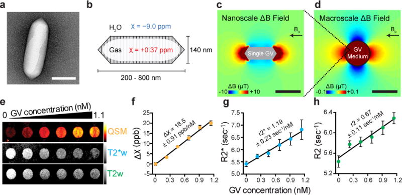
a, Transmission electron microscopy (TEM) image of a GV from Anabaena flos-aquae (Ana) b, Schematic drawing of a GV, whose air-filled interior has magnetic susceptibility (red) different from that of surrounding H2O (blue). c, Finite element model of the magnetic field gradient produced by a single air-filled Ana GV in water exposed to a 7 Tesla horizontal magnetic field (B0). d, Finite element model of the magnetic field gradient produced by a cylindrical sample of 1 nM Ana GVs embedded in an agarose phantom. e, Quantitative susceptibility map (QSM), T2*-weighted (T2*w) and T2-weighted (T2w) images of wells containing Ana GVs at concentrations ranging from 0 to 1.1 nM. The color schemes for QSM (red hot), T2*w (grey) and T2w (grey) images are used across all figures. The QSM color scale ranges linearly from −2 to +50 parts per billion (ppb), and T2*w and T2w images at echo time (TE) = 144 msec have linear scales adjusted for optimal contrast. f, g, h, Magnetic susceptibility, T2* relaxation rate and T2 relaxation rate, respectively for different concentrations of Ana GVs. The value and the standard error of the slope from the linear regression fitting are shown for each plot and corresponds to molar susceptibility (f), r2* relaxivity (g) and r2 relaxivity (h). N = 9 independent samples in (f, g) and N = 6 independent samples in (h). Error bars represent SEM. Scale bars represent 150 nm (a), 300 nm (c) and 3 mm (d).
Air is a well-known source of contrast in MRI due to its positive magnetic susceptibility compared to diamagnetic water, as seen in image artefacts near gas-filled organs such as the lungs13. We reasoned that the air inside GVs would also produce susceptibility-based MRI contrast, which could be observed by T2/T2*-weighted imaging and quantitative susceptibility mapping (QSM). Additionally, because GVs can be collapsed with acoustic pressure12, 14, we hypothesized that the MRI contrast produced by GVs could be erased remotely in situ using ultrasound, an orthogonal non-invasive modality. Such acoustically modulated reporters would overcome a major challenge in MRI posed by background contrast from endogenous sources15 by allowing reporters to be identified specifically based on their acoustic responses. Moreover, this imaging mechanism would be complementary to other recent uses of GVs14, 16, creating possibilities for multimodal imaging. In this study, we set out to test these fundamental hypotheses through in vitro and in vivo experiments and computational modelling. In addition, we sought to demonstrate that the unique material properties of GVs could enable multiplexed, functional and genetically encoded molecular imaging.
GVs produce susceptibility-based MRI contrast at sub-nanomolar concentrations
To assess the ability of GVs to produce susceptibility-based MRI contrast, we performed computational modelling and in vitro imaging experiments. The air contents of the GV interior have an expected magnetic susceptibility of +0.37 ppm, differing significantly from water, which is diamagnetic at −9.0 ppm (Fig. 1b). As a result of this mismatch, individual GVs in aqueous media under a uniform magnetic field are predicted by finite element modelling to produce nanoscale magnetic field gradients (Fig. 1c). The proton nuclear spins on water molecules experiencing such gradients are expected to dephase, leading to enhanced T2/T2* relaxation and a concomitant reduction of local signal intensity in T2- and T2*-weighted images, which can be acquired with widely used spin-echo and gradient-echo MRI pulse sequences17. In addition, macroscale volumes containing GVs have a different average susceptibility than surrounding voxels, producing macroscale field gradients (Fig. 1d), which should cause a patterned change of spin phase beyond the site of the GVs (Supplementary Fig. 1). These phase changes can be decoded by QSM algorithms to produce contrast maps with additional sensitivity beyond magnitude-only T2/T2* images18, 19.
To test the ability of GV nanostructures to produce these forms of contrast, we purified GVs from the cyanobacterium Anabaena flos-aquae (Ana GVs) and imaged them in agarose phantoms with a 7 Tesla MRI scanner. As predicted, GVs produced robust contrast in T2*- and T2-weighed images and QSM maps (Fig. 1e). Quantification of this MRI contrast revealed T2* and T2 relaxivities of 1.19 ± 0.23 nM−1 s−1 and 0.67 ± 0.11 nM−1 s−1, respectively, and molar susceptibility of 18.53 ± 0.91 parts-per-billion (ppb) nM−1 (Fig. 1 f-h and Supplementary Table 1), wherein the nanomolar concentration refers to GV particles. The lowest tested concentration of Ana GVs, at 230 pM, or 73 μg/mL protein, was readily detectable by QSM (p = 0.0014, unpaired t-test, the first two data points of Fig. 1f, degrees of freedom (df) = 11.86). This protein concentration is within the range of other protein-based MRI reporters such as haem-containing cytochromes, ferritin, aquaporin and chemical exchange saturation transfer polypeptides20. At these concentrations, GVs produce negligible T1 contrast (Supplementary Fig. 2), and have an insignificant effect on proton density due to water exclusion (< 0.1 % v/v), preserving these contrast modes for use by orthogonal reporters or anatomical imaging. GVs purified from Halobacterium salinarum NRC-1 (Halo GVs) and GVs formed by expressing a GV gene cluster from Bacillus megaterium in Escherichia coli (Mega GVs) produced similar contrast to Ana GVs (Supplementary Fig. 2).
Background-free acoustically modulated imaging
Conventional T2 and T2* contrast agents such as superparamagnetic iron oxide nanoparticles (SPIONs) are widely used in MRI applications such as in vivo cell tracking21. However, the specificity with which they can be detected in biological tissues is sometimes confounded by the presence of background contrast from endogenous sources such as blood vessels and tissue interfaces15. MR pulse sequences and post-processing methods designed to selectively acquire signals only from SPIONs22–24 often sacrifice molecular sensitivity, while alternative imaging approaches such as magnetic particle imaging (MPI) and 19F-MRI lack tissue context25–28. Unlike SPIONs, GVs have a built-in mechanism by which their identity as the source of any given MRI contrast can be ascertained. Namely, the collapse of their gaseous interior under pressure should eliminate GV’s susceptibility mismatch with water (Fig. 2a), allowing GV-specific contrast to be revealed by differential imaging. Importantly, such pressure can be applied remotely using ultrasound, rendering the entire imaging paradigm non-invasive and depth-unlimited.
Figure 2. Background-free acoustically modulated imaging.
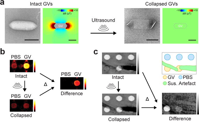
a, TEM images and simulated magnetic field profiles generated by intact and collapsed Mega GVs. Scale bars represent 100 nm. b, Magnetic susceptibility maps of wells containing phosphate-buffered saline (PBS) or 4.9 nM Mega GVs before and after the application of ultrasound, and the resulting difference image. c, T2*-weighted images of a phantom containing wells with 8.1 and 4.9 nM Mega GVs alongside background hyperintense contrast from wells with PBS in low-percentage agarose and hypointense susceptibility artefact from the nearby 40 μm (inner diameter) capillary tubes containing 500 mM NiSO4, before and after the application of ultrasound, and the resulting difference image. The diagram outlines the different regions of the phantom.
We tested this concept by acquiring QSM images of samples containing Mega GVs or buffer before and after acoustic collapse with ultrasound. Subtraction of the pre-collapse image from the image acquired after collapse resulted in background-free contrast specific to the GVs (Fig. 2b). To demonstrate that this method can distinguish GVs from susceptibility artefacts in T2*-weighted imaging, we prepared a phantom containing GVs, regions with lower concentration of agarose and capillary tubes filled with paramagnetic nickel. While GVs are difficult to distinguish from other hyper- and hypo-intense regions in the raw initial image, acoustic collapse and background subtraction enable the specific observation of GVs even at concentrations that were initially difficult to spot by naked eye (Fig. 2c). This differential contrast is positive because GV collapse leads to a longer T2*.
To test the acoustically modulated molecular imaging paradigm in vivo, we began by stereotaxically injecting Ana GVs in the striatum of adult C57 mice and imaging them using T2*-weighted MRI (Fig. 3a). We then collapsed the GVs in situ using brief pulses of MRI-guided focused ultrasound29 and acquired a post-collapse MRI image. The resulting differential image, overlaid on a separately acquired anatomical reference, shows specific background-free contrast from the brain region injected with GVs (Fig. 3b, c). A contralateral injection of phosphate-buffered saline (PBS) without GVs, subjected to the same MRI and ultrasound pulses, produced no significant contrast. The mean collapse-dependent contrast in the GV-injected region was 23.5 ± 3.8% (Mean ± SEM, N = 9) compared to 0.4 ± 2.6% for PBS (Mean ± SEM, N = 6, p = 0.0002, unpaired t-test, df = 12.73). Although we mainly used T2*-weighted images for in vivo background-free imaging due to their convenience, QSM-processed susceptibility maps also visualized GVs with a high contrast-to-noise ratio (Supplementary Fig. 3).
Figure 3. Background-free imaging of GVs in mammalian tissues.
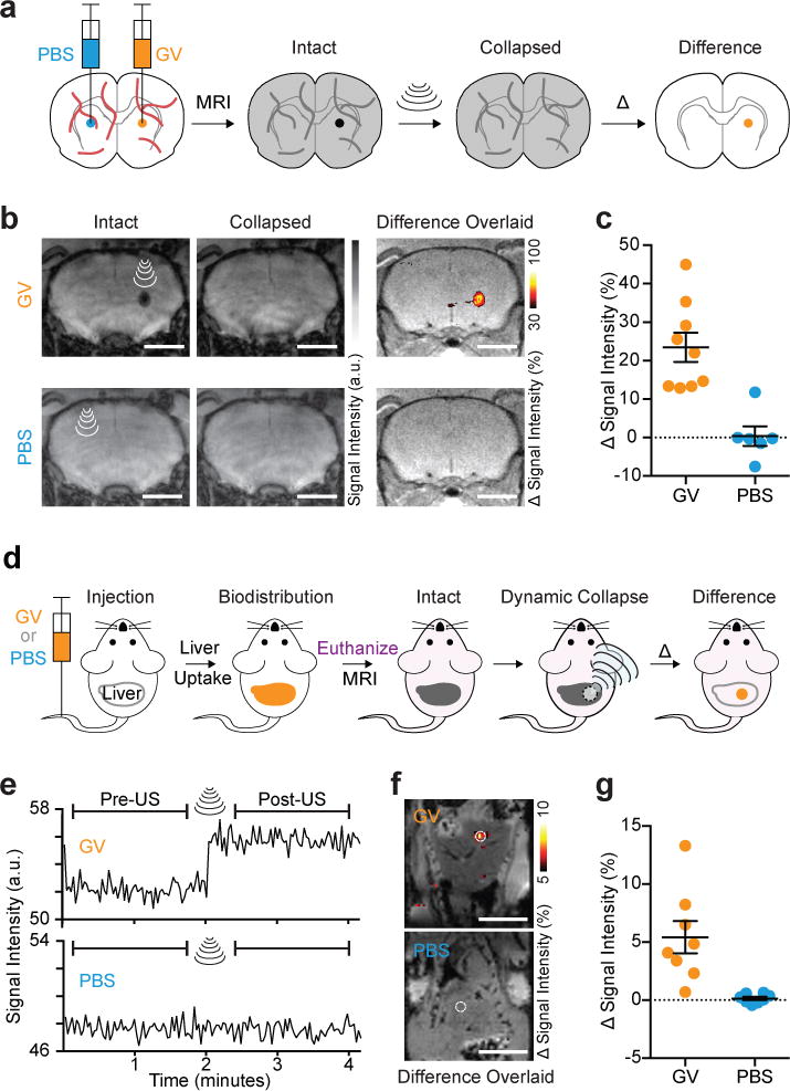
a, Diagram of the in vivo experiment in the living mouse brain. GVs or PBS buffer (sham control) were injected into contralateral striatum. T2*-weighted images taken before the insonation were subtracted from those taken after, and difference images were calculated to reveal contrast specific to the GVs, giving rise to a background-free image. b, Representative T2*-weighted images (TE = 15 msec) of a mouse injected with 2 μL GVs (AnaWT, 3.4 nM) or PBS, acquired before and after ultrasound was applied to the site of injection. The resulting difference images are overlaid on anatomical images. c, Changes in signal intensity upon insonation at the sites of injection (N = 9 and 6 injections for GV and PBS, respectively, in a total of 8 mice) normalized by the intensity of the surrounding brain region. d, Diagram of dynamic imaging of the mouse liver after intravenous administration of GVs. 200 μL PBS with or without 13.7 nM GVs (AnaΔC, clustered form) were injected. After allowing 1 min for the biodistribution of GVs to the liver, mice were euthanized, and T2*-weighted images (1.9 sec/frame) were acquired continuously before, during and after a 5-second application of ultrasound pulses to a spot in the liver. e, Representative time course of signal intensity at an insonated spot (1 mm radius) of mouse liver after intravenous injection with GVs or PBS. f, Difference in intensity between images acquired before and after ultrasound application, overlaid on anatomical images. g, Average signal intensity change in the insonated region upon the application of focused ultrasound to the liver tissue (N = 8 spots for each condition in a total of 8 mice). a.u. denotes arbitrary units. Error bars represent SEM, and scale bars represent 3 mm (b) and 10 mm (e).
Next, we tested the ability of GVs to be imaged in vivo after intravenous (IV) administration. GVs injected into the bloodstream are efficiently taken up by the liver14, a tissue whose ability to clear particles from circulation serves as an important indicator of hepatic health and tumor diagnosis30. Because the liver and surrounding tissues also have high endogenous contrast, hepatic imaging serves as a good test bed for background-subtracted imaging techniques. After administering GVs to mice (Fig. 3d), we performed T2*-weighted imaging before, during and after applying focused ultrasound to the liver. A dynamic jump in average signal intensity in the insonated region was readily observed in mice injected with GVs, but not in mice injected with PBS (Fig. 3e), producing a clear spot of background-subtracted contrast (Fig. 3f). The mean collapse-dependent signal change in the GV-injected mice was 5.4 ± 1.4% compared to 0.1 ± 0.1% for PBS (Mean ± SEM, N = 8, p = 0.0068, unpaired t-test, df = 7.14) (Fig. 3g).
Acoustically modulated imaging of gene expression
After establishing the basic acoustically modulated imaging capabilities of GVs in vitro and in vivo, we tested the ability of these genetically encoded nanostructures to act as reporters of gene expression in living cells. In particular, given the great interest in imaging the mammalian microbiome and bacterial infections31, we assessed whether GVs could image inducible gene expression in the model bacterium E. coli. Heterologous expression of a recently developed GV variant comprising a combination of genes from A. flos-aquae and B. megaterium11 (A2C) was placed under the control of a promoter inducible by isopropyl b-D-1-thiogalactopyranoside (IPTG, Fig. 4a). Overnight induction resulted in GV expression and robust, acoustically erasable QSM contrast that was absent from cells that were not induced or cells induced to express a control fluorescent protein (Fig. 4b, c). Notably, the E. coli concentration in the phantom, estimated from OD600 to be ~ 14 g/L wet cellular weight32, indicates that the GV-containing cells can be detected while comprising less than 1.4 % of the imaged volume.
Figure 4. Acoustically modulated reporter gene imaging in living cells.
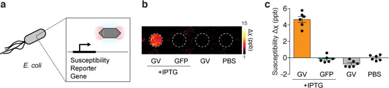
a, Diagram of the inducible expression of GV genes in E. coli leading to the intracellular formation of GVs and the generation of susceptibility-based MRI contrast. b. Representative background-subtracted QSM image of agarose phantom containing E. coli expressing GVs or a green fluorescent protein (GFP) under the control of an IPTG-inducible promoter, in the presence or absence of the inducer, compared to a well containing buffer. c. Mean differential susceptibility values relative to buffer. N = 6 biological replicates. Error bars represent SEM. All bacterial cells were loaded in the phantom at a final OD600 of 8.0.
Acoustically modulated multiplexing
Many imaging applications in biomedicine would benefit from the ability to image multiple molecular or cellular signals in the same tissue33. Because GVs with different protein composition collapse at substantially different acoustic pressures12, 14, this suggests the possibility of performing acoustically modulated imaging in multiplex by collapsing one population of GVs at a time with ultrasound while acquiring a sequence of MR images (Fig. 5a). Voxel-wise intensity changes between successive images should then encode the signal corresponding to each multiplexed GV population.
Figure 5. Acoustically multiplexed magnetic resonance imaging.
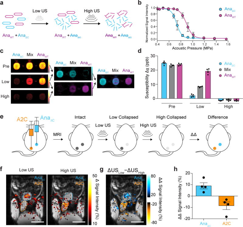
a, Schematic of the pressure-scanning paradigm, wherein sequential ultrasound pulses are applied between MR images. The low-pressure ultrasound (Low US) selectively collapses AnaΔC GVs and eliminates their MRI contrast; subsequently, high-pressure ultrasound (High US) collapses AnaWT GVs. b, Acoustic collapse measurement of AnaΔC and AnaWT. N = 3 independent samples for each point. Fitted curves represent a sigmoid function obtained by nonlinear least-square fitting. c, Representative QSM images taken before ultrasound application (Pre), after the low-pressure ultrasound (Low) and after high-pressure ultrasound (High) of wells containing AnaWT, AnaΔC or a 1:1 mixture of the two, as indicated, followed by difference images obtained by pairwise subtraction, color mapped to distinguish variants collapsing at different pressures, followed by an overlay of the two difference images. The total GV concentrations were 1.37 nM in all three samples and the images were displayed from −10 to +50 ppb. d, Average susceptibility of each sample type relative to PBS buffer at each stage of the pressure-scanning paradigm. N = 4 independent samples. Complete collapse of GV specimens resulted in slightly negative susceptibility relative to the PBS solution, as expected since proteins are more diamagnetic than water. e, Diagram of the in vivo multiplexing experiment in the living mouse lower abdomen. f, Maps of changes in MRI signal intensity in insonated regions overlaid on anatomical MR image. The insonated regions are outlined in white, while the subcutaneously injected areas are outlined in blue or orange, corresponding to their contents. g, Map of the differential change in the change in signal intensity after the application of Low US relative to High US. h, Average signal change at 8 injection sites (4 of each type from a total of 4 mice). a.u. denotes arbitrary units. Error bars represent SEM (b, d, h), and scale bars represent 10 mm (f, g).
GVs with different collapse pressures can be obtained by isolating genetically distinct variants or by modifying their shell12. Here, we used a variant of Ana GVs (referred to as AnaΔC) whose acoustic collapse pressure has been lowered by removing its outer scaffolding protein, GvpC12 (Fig. 5b). Since GvpC removal does not alter the morphology of the GV, AnaΔC produces MRI contrast equivalent to wildtype Ana GVs (AnaWT). To demonstrate multiplexing, we prepared a phantom with three wells containing AnaΔC, AnaWT and a 1:1 mixture (Fig. 5c). We then acquired three sequential MR images interspersed by ultrasound pulses at AnaΔC- and AnaWT-collapsing pressures. Changes in the measured magnetic susceptibility of each voxel between the relevant pairs of images revealed the contents of each sample (Fig. 5, c-d).
Next, to test the multiplexing paradigm and demonstrate the imaging of bacterial gene expression in vivo, we injected AnaΔC GVs and E. coli cells expressing A2C GVs subcutaneously and acquired sequential MR images interspersed by ultrasound pulses selectively collapsing, first AnaΔC GVs, then A2C GVs, at each location (Fig. 5e). Difference images revealed significant signal for AnaΔC GVs only upon low-pressure collapse, since few GVs were left intact to be collapsed at high pressure (Fig. 5f and Supplementary Fig. 4). In contrast, E. coli expressing the more mechanically robust A2C GVs produced a signal change specifically in response to higher pressure. Subtracting the signal change generated by low-pressure ultrasound from the change generated by high-pressure ultrasound enables quantitative assignment of the contrast source (Fig. 5, g-h). AnaΔC GVs and A2C-expressing E. cells yield positive and negative values, respectively, with +9.0 ± 2.7% for AnaΔC and −8.5 ± 3.3% for A2C GVs (Mean ± SEM, N = 4, p = 0.0072, unpaired t-test, df = 5.73).
Multiparametric MRI multiplexing
In addition to acoustic multiplexing, we hypothesized that GVs with different shapes and sizes could be distinguished on the basis of their differential effects on T2 and QSM contrast. GV morphology should alter the nanoscale magnetic field patterns generated by a given quantity of gas, affecting T2 relaxation34. In contrast, the magnetic susceptibility calculated from QSM is expected to depend on the total amount of gas in the sample, independent of its nanoscale arrangement. Each type of GV should therefore have its own parametric fingerprint. We tested this hypothesis using Ana GVs, GVs purified from E. coli expressing a GV gene cluster from Bacillus megaterium (Mega)10 and GVs purified from Halobactrium salinarum (Halo) (Fig. 6a). After measuring the T2 relaxivity and molar susceptibility values for each molecule (Fig. 6a, Supplementary Fig. 2), we used Mega and Halo GVs to demonstrate multiplexed imaging. Each GV type had a distinct appearance under susceptibility contrast relative to its T2 relaxivity (Fig. 6b), and voxel-wise unmixing of susceptibility (Δχ) and relaxation rate (R2) according the equation
| (1) |
revealed the quantities of the two GV types in each sample, Cα and Cβ (Fig. 6c). This multiparametric MRI paradigm35 has the advantage of being non-destructive compared to acoustic multiplexing, but is statistically less accurate (Supplementary Fig. 5).
Figure 6. Multiparametric MRI fingerprinting and clustering-based molecular sensors.
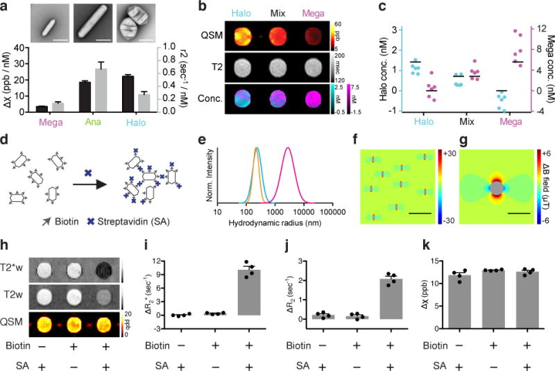
a, TEM images and magnetic susceptibility and r2 relaxivitiy values for Mega, Ana and Halo GVs. The molar susceptibility (Δχ) values are referenced to blank PBS buffer. Error bars represent the standard error of the slope from linear regression fitting (Supplementary Fig. 2). b, Representative susceptibility map (QSM), T2 relaxivity map (T2) and calculated GV concentrations (Conc.) of three samples that contain Halo GVs, Mega GVs or a 1:1 mixture of both GV types. The concentration of Mega (magenta) and Halo (cyan) GVs were pixel-wise calculated and displayed in overlay. c, GV concentrations calculated from MRI images in N = 6 independent samples. Black bars represent the expected GV concentration. d, Diagram of the clustering experiment using biotinylated Ana GVs and streptavidin (SA). e, Dynamic light scattering (DLS) measurement of the size distributions of biotinylated GVs with SA (magenta), biotinylated GVs without SA (cyan) and non-biotinylated GVs with SA (orange). f, g, Finite element model of the magnetic field pattern expected from individual (f) and clustered (g) GVs. Scale bars represent 2 μm (f) and 4 μm (g). h, Representative T2*-weighted (T2*w) and T2-weighted (T2w) images and QSM maps of agarose phantom wells containing GVs with the indicated biotinylation state and presence or absence of SA. i, j, k, Average change in R2* (i), R2 (j) and χ (k) relative to PBS buffer. N = 4 independent samples. Error bars represent SEM. All the GV samples contained Ana GVs at 0.57 nM.
Clustering-based molecular sensors
In addition to contrast agents reporting their location, there is considerable interest in the development of dynamic molecular sensors36–39. For example, superparamagnetic nanostructures that cluster in response molecular signals of interest can increase or decrease T2 or T2* contrast36, 39, 40. We hypothesized that GVs would also produce differential MRI contrast based on clustering. In particular the size and magnetic character of GVs places them in the so-called motional averaging regime34, 41–43 of T2/T2* relaxation, such that their clustering in response to a target analyte should result in an increase in both T2* and T2 relaxivity. We tested this hypothesis using biotin-functionalized Ana GVs mixed with tetrameric streptavidin (Fig. 6d and Supplementary Fig. 6). At appropriate streptavidin concentrations, GVs form micron-size clusters (Fig. 6e), predicted to produce a magnetic field profile with correspondingly large spatial dimensions (Fig. 6f-g). Upon clustering, T2*- and T2-weighted images showed dramatic relaxation enhancement compared to controls lacking biotinylation or streptavidin (Fig. 6h), with R2* and R2 increasing approximately 15- and 5-fold, respectively (Fig. 6i-j). Remarkably, the QSM image was largely unaltered (Fig. 6k), as expected given the conservation of total air between the three samples; this allows a change in clustering to be distinguished from an increase in the number of particles, thereby enhancing sensing robustness.
Outlook
Our results establish GV as protein-based acoustically modulated MRI contrast agents, using the combination of ultrasound and MRI to enable background-free and multiplexed molecular imaging. This imaging modality takes advantage of the material properties of GVs, including both, the magnetic susceptibility of their interior as a perturbation of the magnetic field in liquid media, and the mechanics of their protein shell allowing collapse at specific acoustic pressures. Acoustically modulated reporters should be particularly useful in imaging scenarios with confounding background contrast15, 44–46.
The distinct size, shape and mechanical properties of genetic variants of GVs provide opportunities for future molecular engineering. For example, GV morphology could be optimized to maximize spin dephasing and T2/T2* contrast, or to facilitate multiplexing of several GV types on the basis of differential relaxivity. At the same time, engineering GV shells with a greater variety of critical collapse pressures could expand multiplexing ability using acoustic collapse. Between these two modes of multiplexing, non-acoustic multiplexing has the advantage of not requiring an ultrasound system. However, the acoustic approach is more accurate in distinguishing GV concentrations, and is independent of the microscale spatial arrangement of GVs. Genetic or chemical engineering of the GV shell12, 47 also provides a route to designing targeted MRI reporters and sensors, the delivery of which may be facilitated by engineering GVs with smaller sizes9, 48. In parallel, engineered genetic circuits incorporating GV reporter genes could be used to image bacteria in vivo.
Several limitations must be addressed in future studies to establish the wider applicability of GVs as acoustically modulated susceptibility contrast agents. First, while the three mouse experiments presented in this study provide proofs of concept for the in vivo implementation of acoustically modulated GV imaging, additional work is needed to demonstrate applications of this technique in biomedically useful scenarios. Such applications could include evaluating hepatic health by imaging the uptake of intravenously injected GVs, labelling specific endothelial or extra-vascular biomarkers or monitoring bacterial biodistribution. To facilitate such applications, additional experiments are needed to establish the tolerability and immunogenicity of injected GVs. Mice injected with repeated doses of GVs over several days in our study did not exhibit any behavioural abnormality, consistent with previous veterinary assessments14. However, more detailed histological and biochemical studies are needed.
In addition, the acoustically modulated imaging protocol can be simplified to replace focused ultrasound with an unfocused source, allowing larger areas of the specimen to experience GV collapse. Unlike ultrasound imaging, which requires sound wave coherence for image reconstruction, acoustically modulated MRI only requires enough ultrasound pressure to reach tissues to collapse GVs, facilitating transmission through bone and providing flexibility in instrument design. Finally, the expression of GVs is currently limited to bacterial hosts. Making mammalian cells capable of producing GVs is an active area of ongoing research.
Together with other recent literature, this study establishes GVs as a tri-modal imaging agent. GVs have recently been explored for ultrasound imaging based on their ability to scatter sound waves14, and for hyperpolarized 129Xe CEST imaging based on the ability of xenon gas to exchange across the GV shell16. Compared with pulse-echo ultrasound, acoustically modulated MRI has an advantage in accessing bone-enclosed structures such as the brain. It is also much simpler to implement than hyperpolarized 129Xe imaging, which requires specialized procedures for gas hyperpolarization and delivery. Nevertheless, the ability of GVs to be visualized with multiple modalities increases their appeal as a molecular imaging nanomaterial.
METHODS
Expression and purification of gas vesicles
Ana and Halo GVs were purified after expression in their respective host bacteria. Anabaena flos-aquae (CCAP strain 1403/13F) was cultured in Gorham’s media supplemented with BG-11 solution (Sigma, St. Louis, MO) and 10 mM NaHCO3 at 25°C, 100 rpm shaking and 1% CO2 under a 14 h-light-10 h-dark cycle and confluency was reached in ~ 2 weeks. Halobacteria NRC-1 (Carolina Biological Supply, Burlington, NC) were cultured at 42°C in ATCC medium 2185 under ambient light and with shaking at 100 rpm. Confluency was reached in ~ 1 week. Both types of cultures were transferred to sterile separating funnels. The buoyant cells were allowed to float to the top over a 48 h period. The subnatant was discarded and the floating cells were collected. Anabaena cells were lysed with 500 mM sorbitol and 10% Solulyse solution (Genlantis, San Diego, CA), and Halobacteria cells were hypotonically lysed with the addition of excess low-salt TMC buffer (10 mM Tris, pH = 7.5, 2.5 mM MgCl2, 2mM CaCl2). GVs were separated from cell debris by repeated centrifugally assisted floatation followed by resuspension in 1x PBS (Teknova, Hollister, CA). The centrifugation speed was carefully controlled to avoid the hydrostatic collapse of GVs. To prepare solution for in vivo experiments, purified GVs were dialyzed overnight in 1 × PBS solution. The concentration of gas vesicles (GVs) was estimated based on the pressure-sensitive optical density at 500 nm (OD500,PS) due to the ability of intact GVs to scatter light8.
AnaΔC was prepared by treating Ana GVs with a solution of 6 M urea and 20 mM Tris-HCl (pH = 8.0). Two rounds of centrifugally assisted buoyancy purification were performed to remove GvpC. The solution was then dialyzed overnight in 1 × PBS buffer to remove urea.
GVs from Bacillus megaterium (Mega) were heterologously expressed in E. coli Rosetta™ 2(DE3)pLysS (EMD Millipore, Billerica, MA). The pNL29 region of the Mega GV gene cluster10 was cloned into the pST39 plasmid for expression under the control of the T7 promoter16. The transformed cells were grown at 30°C in LB media supplemented with 0.2% glucose. 20 μM isopropyl β-D-1-thiogalactopyranoside (IPTG) was added at OD600 between 0.4 and 0.6 to induce the expression of GVs, and the cells were grown overnight before harvesting by centrifugation. The clear subnatant was removed by a syringe, while both the floating and the pelleted cells were collected. The cells were lysed in 10% Solulyse (Genlantis, San Diego, CA), 250 μg/ml lysozyme and 10 μg/ml DNaseI. Centrifugally assisted floatation and OD500 measurement followed the procedure used for Halo and Ana GV. Mega GVs, which are natively clustered after purification from bacteria, were unclustered using the same urea treatment, buoyancy purification and dialysis procedure described for the preparation of AnaΔC GVs. Gas vesicle concentrations were determined using the relationships summarized in Supplementary Table 147.
Reporter gene expression
For reporter gene experiments, the gene cluster encoding a hybrid GV variant named A2C11 was cloned into pET28a plasmid (Novagen, Temecula, CA), and the resulting plasmid was transformed into BL21(A1) cells (Thermo Fisher Scientific, Waltham, MA). The transformed cells were first grown overnight at 30°C in LB media supplemented with 1% glucose, and this starter culture was subsequently diluted 1:100 into LB media supplemented with 0.2% glucose. When OD600 reached between 0.4 and 0.6, 400 μM IPTG and 0.5% arabinose were added to induce expression of GVs. The control green fluorescent protein mNeonGreen49 was inserted into the same plasmid and followed the identical culturing protocol.
Cell density was measured after collapsing any intracellular GVs to eliminate their contribution to optical scattering (Supplementary Fig. 7). A sample of each E. coli specimen at OD600 ~ 1.0 was loaded onto a flow-through, 1 cm path-length quartz cuvette (Hellma Analytics, Plainview, NY), which was pressurized by an N2 cylinder and a digital pressure controller (Alicat Scientific, Tucson, AZ). The pressure was incremented in 20 kPa steps from 0 to 1.2 MPa and OD600 was recorded using a spectrophotometer (EcoVis, OceanOptics, Winter Park, FL). OD600 at 1.2 MPa was used to measure cell density. Prior to the preparation of MRI phantoms, the cells were concentrated by centrifugation to the indicated density. For in vivo imaging, the buoyant fraction of cells was concentrated and collected after several rounds of centrifugation at 350 g (4 hrs).
Transmission electron microscopy (TEM)
GVs at OD500,PS ~ 0.2 were prepared in a buffer of 10 mM HEPES, 150 mM NaCl (pH 8) and spotted on Formvar/Carbon 200 mesh grids (Ted Pella) that were rendered hydrophilic by glow discharging (Emitek K100X). GV samples were negatively stained using 2% uranyl acetate. Images were acquired using a Tecnai T12 LaB6 120kV TEM.
In vitro MRI and relaxometry
Purified GVs or E. coli cells were embedded in agarose phantoms. 1% agarose stock solution was prepared in PBS and maintained at 60°C until use. The size of the phantom was ~ 18 × 6 × 4 cm (length × width × height). Using a custom 3D-printed caster, the bottom half was first cast with cylindrical wells of the size 3 × 5 mm (diameter × depth) separated by 3 mm. The cylindrical geometry perpendicular to B0 was chosen to ensure a homogeneous field in the sample wells to facilitate susceptibility-based imaging. The gel was allowed to solidify and exposed to air for 1 h for gas equilibration. Two-times concentrated GVs or E. coli cells in PBS were mixed 1:1 with the melted agarose stock solution and immediately loaded into the wells. Subsequently, the top half of the phantom was cast so that all the wells were surrounded by agarose. Care was taken to avoid bubbles.
MRI was performed on a 7T horizontal bore Bruker-Biospin scanner, using a 7.2 cm diameter volume coil for transmit and receive. T2* relaxivity was measured with 3D Multi Gradient Echo (MGE) experiments with the following parameters: repetition time (TR) = 500 ms, 32 echos, echo spacing (TE) = 9.0 ms, field of view (FOV) = 12 × 6 × 0.8 cm3, spatial resolution = 0.25 × 0.25 × 0.25 mm3 and 1 average. T2 relaxometry was performed by 2D Multi Slice Multi Echo (MSME) spin echo experiments with the following parameters: TR = 2500 ms, 16 echos, TE = 16.0 ms, FOV = 8 × 6 cm2, and spatial resolution = 0.25 × 0.25 mm2. Slice thickness = 1 mm and 16 averages were used for multiparametric multiplexing experiments and 0.5 mm and 4 averages for all other experiments. T1 relaxometry was performed by 2D Rapid Acquisition with Relaxation Enhancement with Variable TR (RAREVTR) with the following parameters: Effective TE = 9.68 ms, RARE factor = 12, FOV = 8 × 6 cm2, spatial resolution = 0.25 × 0.25 mm2, slice thickness = 0.5 mm, 2 average and 8 variable TR times including: 126.4, 738.4, 1461.2, 2344.1, 3478.7, 5068.5, 7746.6, 20000.0 ms.
For data analysis, a circular region of interest (ROI) was drawn for each well using Fiji50. The average intensity of the ROI was imported into Matlab for exponential fitting to derive the T2*, T2 and T1 values. Voxel-wise T2* and T2 maps were generated by ImageJ plugin, MRI Processor, using Simplex fitting. For T2* relaxometry, the ROI excluded the rim of the wells. Multiparametric multiplexing of GVs was achieved by solving the matrix equation:
| (1) |
where the concentrations of the two GV species, cα and cβ, were the two unknowns. r2,α and r2,β were the r2 relativity and Δχm,α and Δχm,β were the molecular susceptibility of the GVs, and and were the experimentally measured relaxation rate and susceptibility (Supplementary Table 1).
Quantitative susceptibility mapping
Magnitude and phase images of 3D MGE or 3D fast low angle shot (FLASH) experiments were obtained in ParaVision 5.1 (Bruker), and the images from a single echo served as the input to the Susceptibility Mapping and Phase artifacts Removal Toolbox (SMART) (MRI Institute for Biomedical Research, Detroit, MI). This software performed phase unwrapping using the 3D-SRNCP algorithm51, background field removal by the SHARP algorithm52 and susceptibility map generation using the SWIM algorithm53. The resulting QSM images were analyzed in Fiji50. Unless specified otherwise, all QSM images were processed from the 5th echo (TE = 45.0 ms) of a 3D MGE experiment.
Gas vesicle clustering
Purified Ana GVs were biotinylated using a 105 molar excess of EZ-Link Sulfo-NHS-LC-biotin (Thermo Scientific, Rockford, IL) for 4 hours in PBS buffer. The excess biotin was removed by two rounds of overnight dialysis in PBS buffer. Biotinylated or control GVs at OD500,PS = 10 were incubated with streptavidin (Geno Technology, St. Louis, MO) at the ratio specific to each experiment for 30 minutes at room temperature before loading into MRI phantom. Dynamic light scattering measurements were performed using a Zeta-PALS instrument (Brookhaven Instruments, Hotsville, NY) at a concentration equivalent to OD500,PS = 0.2 in PBS.
In vitro acoustic collapse
Acoustic GV collapse was performed outside the MRI scanner for in vitro experiments. Multiplexing experiments were performed with a single element immersion transducer (Olympus) with transmit frequency = 2.25 MHz, element size = 0.75 inch, focal length = 1.5 inch, pulse duration = 10 μs, duty cycle = 0.1 %. A waveform generator (Model WS8352, Tabor Electronics, Tel Hanan, Israel) and a power amplifier (Model 3100LA, Electronics & Innovation, Rochester, NY) were used to drive the transducer. The input voltages to the transducer were 57 V and 131 V for collapsing AnaΔC and AnaWT GVs in the agarose phantom, respectively. The output peak positive pressures were estimated by a fiber optic hydrophone (Precision Acoustics, Dorchester, UK) to be 0.74 MPa and 1.41 MPa, respectively. For collapsing the intracellular GVs in E. coli, a Verasonics Vantage programmable ultrasound scanning system using the L11-4v 128-element linear array transducer (Verasonics, Kirkland, MA) was used with the following parameters: transmit frequency = 6.25 MHz, transmit voltage = 15 V.
Acoustic collapse curves were measured with ultrasound as described previously12. Briefly, AnaΔC at OD500 = 1, AnaWT at OD500 = 1, buoyancy-enriched A2C-expressing E. coli at OD600 = 1, and clustered AnaΔC at OD500 = 0.5 (measured prior to clustering) were prepared in agarose phantoms. An 128-element linear array transducer (L22-14v, Verasonics, Kirkland, MA) was used at f-number 2.0 to collapse GVs, and to determine the intact fraction via backscattered ultrasound signal intensity. A ray line script with 15.625 MHz transmit frequency was used for both collapsing GVs and acquiring ultrasound images. To achieve uniform collapse at each acoustic pressure, a mechanical motor system was used to move the transducer over a 6-mm vertical distance at the speed of 0.2 mm/sec for 6 repetitions to cover the depth of the agarose well. In addition to the imaging plane, two additional planes spaced ± 300 μm along the azimuth were subjected to acoustic collapse to ensure completeness. Transducer output pressure was calibrated by a fiber optic hydrophone (Precision Acoustics, Dorchester, UK).
In vivo injections, MRI and acoustic collapse
All animal experiments were approved by the Institutional Animal Care and Use Committee (IACUC) of the California Institute of Technology. Animals were randomized between experimental groups; blinding was not necessary. Mice were anaesthetized using 1 - 2.5% isoflurane in all the injection procedures. For intracranial injection, 2 μL PBS buffer with or without 3.4 nM AnaWT GVs was injected into the striatum or the thalamus of male C57BL6J mice between 12 and 18 weeks of age (Jackson Laboratory, Bar Harbor, ME) using a Nanofil blunt-end g35 needle coupled with a motorized pump (World Precision instruments, Sarasota, FL) at 100 nL/min using a stereotaxic frame (Kopf, Tujunga, CA). The coordinates of the two pairs of sites with respect to the bregma were: +1 mm anterior-posterior, ±2 mm medio-lateral, −3.25 to −3.5 mm dorso-ventral and −2.5 mm anterior-posterior, ±1.5 mm medio-lateral, −3.25 mm dorso-ventral. The needles remained in place after injection for 5 minutes to avoid backflow along the needle tract. OD500,PS of the GV solution inside the syringe was measured post-injection to confirm GV integrity. For intravenous injection, female Nu/J mice 8-20 weeks of age (Jackson Laboratory, Bar Harbor, ME) were infused with 200 μL PBS buffer with or without clustered AnaΔC (13.7 nM, measured before clustering) using 29G syringe (BD, Franklin Lakes, NJ) at a flow rate of 75 μL/min. The mice were euthanized by cervical dislocation 1 minute after the end of infusion to enable imaging of the liver without respiratory motion artefacts. For multiplexing experiments, PBS solution containing clustered AnaΔC (13.7 nM, measured before clustering) or E. coli cells expressing A2C GVs (OD600 = 150 measured without collapse) were chilled on ice and mixed 1:1 v/v with Matrigel HC (Corning Inc., Corning, NY), then injected subcutaneously into the lower abdomen of female Nu/J mice 8-20 weeks of age using 21G syringes in volumes of approximately 200 μl before live-animal imaging.
For imaging, live mice were anaesthetized using 1-2% isoflurane and were placed in an acrylic cradle where respiration and body temperature were continuously monitored using a pressure transducer (Biopac Systems) and fiber optic rectal thermometer (Neoptix). Warm air was circulated to maintain body temperature at 30°C. For brain imaging, a 72 mm diameter volume coil was used for RF transmission and a 30 mm diameter surface coil for detection. T2*-weighted images were acquired by 2D or 3D FLASH experiments with the following parameters: TE = 15.0 ms, TR = 50.6 ms, flip angle = 20°, FOV = 40 × 28 mm2, spatial resolution = 0.1 × 0.1 mm2, slice thickness = 1.0 mm and 64 averages (2D) or 64 averages and 1 average (3D). Anatomical images were acquired by 2D RARE experiments with the following parameters: effective TE = 19.98 ms, RARE factor = 8, TR = 300 ms, FOV = 140 × 512 mm2, spatial resolution = 0.1 × 0.1 mm2, slice thickness = 1.0 mm and 1 average. For liver imaging, 2D FLASH experiments were repeated at the rate of 1.9 sec per image with the following parameters: TE = 8.0 ms, TR = 23.4 ms, flip angle = 21°, FOV = 64 × 40 mm2, spatial resolution = 0.5 × 0.5 mm2, slice thickness = 2.5 mm and 1 averages. For multiplexing experiment, 3D MGE experiments were performed with the following parameters: TR = 46.8 ms, 8 echos, first echo time 3.66 ms, TE = 4.78 ms, FOV = 128 × 40 × 48 mm3, spatial resolution = 0.5 × 0.5 × 0.5 mm3 and 1 average. The T2*-weighted images from the 7th echo (TE = 32.3 ms) were used to calculate the change of intensity upon acoustic collapse.
In situ collapse of GVs was achieved using an MRI-guided focused ultrasound system comprising an 8-channel signal generator, a motorized MRI-compatible transducer positioning system and an annular array transducer operating at 1.5 MHz (Image Guided Therapy, Pessac, France). For brain imaging, two ultrasound pulse schemes were used to transcranially collapse Ana GVs, with the following parameters: (1) pulse length (PL) = 10 μs, duty cycle = 0.01 %, peak positive pressure (PPP) = 5.7 MPa, 10 to 200 shots; (2) PL = 50 ms, duty cycle = 5 %, PPP = 3.0 MPa, 100 to 600 shots. Both schemes were capable of collapsing GVs and were tested for both the GV and the control PBS injection sites. For liver imaging, focused ultrasound pulses were applied at a single lateral position, with 5 axial spots 1 mm apart from each other (using electronic focusing without movement of the transducer) using the following parameters: PL = 10 μs, duty cycle = 0.1%, PPP = 2.3 MPa and 100 shots for each spot. For multiplexing experiments, regions of interest sized 3.5 × 5 mm or 5 mm × 5 mm laterally were insonated at an average lateral density of 7 focal spots per mm2. Each lateral spot received 1 or 2 pulses at each of 6 different electronically focused axial depths, set apart by 1 mm. The pulse parameters were PL = 1 ms, duty cycle = 5%, PPP = 1.3 MPa for AnaΔC and PPP = 3.2 MPa for A2C. All PPPs were measured by a fibre optic hydrophone (Precision Acoustics, Dorset, UK) in degased water. 18% attenuation was assumed for the mouse skull54 in brain imaging, and no attenuation was assumed for the other experiments.
Data analysis was performed in Fiji50. For brain imaging quantification, an elliptical ROI was manually drawn for the hypointense region containing GVs. Another concentric ROI with twice the radius was drawn, and the intensity of the region between the two ROI was used to measure the intensity of the background tissue. The intensity of the GV region normalized by the background was used to calculate the percentage contrast change upon ultrasound exposure. For liver imaging, a circular ROI of 1 mm in radius was drawn at the focal point of the ultrasound for quantification. To obtain the difference images, 50 frames of the 2D-imaging sequence acquired before and after ultrasound application were averaged, and the post-collapse average was subtracted from the pre-collapse average. For quantification, the average intensity change of the pixels within each ROI was divided by that of the post-collapse image, resulting in the percentage signal intensity change. For the multiplexing experiment, images acquired after ultrasound application (averages of 3 neighbouring planes reconstructed from 3D imaging) were subtracted from the immediately preceding images, and ROIs were drawn corresponding to the insonated areas. To normalize the signal intensity of pre- and post-collapse images, the average intensity of the pixels in an oval area of 20 × 28 mm (width × length) that encompassed the majority of the mouse body was first subtracted from that in each ROI before the change of signal intensity within ROIs upon insonation was calculated. To obtain the percentage of the ΔΔ signal intensity, the average intensity change of the pixels within each ROI was divided by that of the post-collapse image, and the resulting percentage of Δ signal intensity of low-pressure insonation was subtracted by that of high-pressure insonation.
Finite element simulations
The magnetic field simulation was performed in Finite Element Method Magnetics (FEMM) version 4.2 (ref55). GVs were simulated as an axisymmetric object with its longitudinal axis aligned parallel to the magnetic field. The ratio of the susceptibility between inside and outside (χin/χout) of the GVs was taken to be 1 + 9.395 ×10⁻⁶, which corresponds to the susceptibility difference between air and water. For the inside of the cylindrical well, GVs were assumed to be homogenously distributed, and the ratio of the susceptibility between inside and outside of the well (χin/χout) was set to be 1 + 3.426 × 10⁻⁸, which was the volume-weighted average for 0.36% air in water, the amount expected for 1 nM concentration of Ana GVs. Then the cylindrical well in an agarose phantom was simulated as a circle in a 2D planar domain. Similarly, the GV cluster was simulated as a single sphere in the axisymmetric domain occupying a volume equivalent of 200 GVs packed at 20% density and χin/χout of 1 + 1.879 ×10⁻⁶ for 20% air. In all cases, the external field was set at 7.0 T to correspond to the experimental condition.
Monte Carlo simulation for multiplexing accuracy
The simulation was performed in MATLAB, with N = 100 points simulated for each condition. For simple acoustic multiplexing (Supplementary Fig. 6a), the apparent concentration of each GV type was calculated from simulated data using the simple multiplexing assumptions that all GVs of type α were collapsed by low-pressure ultrasound, while all GVs of type β were collapsed only by high-pressure ultrasound. Under this assumption of complete segregation, the molar concentration of the two types of GVs, cα and cβ, was calculated as:
| (2) |
| (3) |
where Δχm,α and Δχm,β were the molecular susceptibilities of GVs of types α and β (Supplementary Table 1), and and were the simulated experimental measurements of susceptibility change upon the application of low-pressure and high-pressure ultrasound. These values were simulated according to:
| (4) |
| (5) |
fα,low, fα,high, fβ,low and fβ,high were values corresponding to the fractions of GV types α and β that were collapsed specifically upon the application of low- and high-pressure ultrasound with the assumption that fα,low + fα,high = 1 and fβ,low + fβ,high = 1, and δfα,low and δfβ,low were random numbers generated based on the standard deviations of the collapsed fractions of AnaΔC and AnaWT at low-pressure ultrasound (Fig. 5b), assuming high-pressure ultrasound was sufficiently strong to collapse all GVs. δχlow and δχhigh were independent random numbers generated according to the standard deviation observed in regression fitting of Δχ measurements (Supplementary Fig. 1a).
Note that, in reality, a fraction of GV type β collapses at the low pressure, while a fraction of GV type α is left over to be collapsed at the high pressure, leading to a systematic error in the apparent concentration (Supplementary Fig. 6a). This error can be reduced with linear spectral unmixing, which takes into account knowledge of the unique acoustic collapse profile of each GV type12 (Supplementary Fig. 6b). In this case, the apparent molar concentrations of the two types of GVs, cα and cβ, are calculated as:
| (6) |
Finally, for multiparametric multiplexing (Supplementary Fig. 6c), the molar GV concentrations were calculated according to
| (7) |
where r2,α and r2,β were r2 relaxivities of GVs of types α and β, and and were the simulated experimental measurements of R2 and susceptibility of the sample, simulated according to:
| (8) |
| (9) |
where δχ and δR2 were normally distributed random numbers using standard deviations observed in Δχ and R2 measurements. In simulating the multiplexing between Halo and Mega GVs, δχ and δR2 represented weighted averages of the standard deviations for Halo and Mega GVs (Supplementary Fig. 1) according to cα (representing Halo GVs) and cβ (representing Mega GVs).
Statistical Analysis
Sample sizes were chosen on the basis of preliminary experiments so as to have sufficient power for the reported statistical comparisons. Unless stated otherwise, statistical comparisons used two-tailed heteroscedastic t-tests with Welch’s correction.
Supplementary Material
Acknowledgments
We acknowledge Arnab Mukherjee, Pradeep Ramesh, Hunter Davis, Russell Jacobs, Xiaowei Zhang and Michael Tyszka for helpful discussions. AF acknowledges financial support from the Natural Sciences and Engineering Research Council of Canada. AL acknowledges financial support from National Science Foundation. This project was supported by the National Institutes of Health (grant EB018975). MGS also acknowledges funding from the Dana Foundation, the Burroughs Wellcome Career Award at the Scientific Interface, the Packard Fellowship in Science and Engineering and the Heritage Medical Research Institute.
Footnotes
AUTHOR CONTRIBUTIONS
GJL and MGS conceived the study. GJL, AF and JOS, ALG and MGS designed, planned and performed the experiments and analyzed data. SB provided software for QSM analysis. AL and RWB provided reagents. All authors discussed the results. GJL and MGS wrote the manuscript with input from all authors. All authors have given approval to the final version of the manuscript.
COMPETING FINANCIAL INTERESTS
The authors declare no competing financial interests.
DATA AND MATERIALS AVAILABILITY
Raw data, gas vesicles and genetic constructs are available upon request to the authors. MATLAB scripts for Monte Carlo simulations are available at http://shapirolab.caltech.edu/?page_id=525.
References
- 1.Caravan P, Ellison JJ, McMurry TJ, Lauffer RB. Gadolinium(III) Chelates as MRI Contrast Agents: Structure, Dynamics, and Applications. Chem Rev. 1999;99:2293–2352. doi: 10.1021/cr980440x. [DOI] [PubMed] [Google Scholar]
- 2.Weissleder R, et al. Ultrasmall superparamagnetic iron oxide: characterization of a new class of contrast agents for MR imaging. Radiology. 1990;175:489–493. doi: 10.1148/radiology.175.2.2326474. [DOI] [PubMed] [Google Scholar]
- 3.Genove G, DeMarco U, Xu H, Goins WF, Ahrens ET. A new transgene reporter for in vivo magnetic resonance imaging. Nat Med. 2005;11:450–454. doi: 10.1038/nm1208. [DOI] [PubMed] [Google Scholar]
- 4.Cohen B, Dafni H, Meir G, Harmelin A, Neeman M. Ferritin as an Endogenous MRI Reporter for Noninvasive Imaging of Gene Expression in C6 Glioma Tumors. Neoplasia. 2005;7:109–117. doi: 10.1593/neo.04436. [DOI] [PMC free article] [PubMed] [Google Scholar]
- 5.Gilad AA, et al. Artificial reporter gene providing MRI contrast based on proton exchange. Nat Biotech. 2007;25:217–219. doi: 10.1038/nbt1277. [DOI] [PubMed] [Google Scholar]
- 6.Zhang S, Merritt M, Woessner DE, Lenkinski RE, Sherry AD. PARACEST Agents: Modulating MRI Contrast via Water Proton Exchange. Acc Chem Res. 2003;36:783–790. doi: 10.1021/ar020228m. [DOI] [PubMed] [Google Scholar]
- 7.Taratula O, Dmochowski IJ. Functionalized 129Xe contrast agents for magnetic resonance imaging. Curr Opin Chem Biol. 2010;14:97–104. doi: 10.1016/j.cbpa.2009.10.009. [DOI] [PMC free article] [PubMed] [Google Scholar]
- 8.Walsby AE. Gas vesicles. Microbiological Reviews. 1994;58:94–144. doi: 10.1128/mr.58.1.94-144.1994. [DOI] [PMC free article] [PubMed] [Google Scholar]
- 9.Pfeifer F. Distribution, formation and regulation of gas vesicles. Nat Rev Micro. 2012;10:705–715. doi: 10.1038/nrmicro2834. [DOI] [PubMed] [Google Scholar]
- 10.Li N, Cannon MC. Gas Vesicle Genes Identified in Bacillus megaterium and Functional Expression in Escherichia coli. J Bacteriol. 1998;180:2450–2458. doi: 10.1128/jb.180.9.2450-2458.1998. [DOI] [PMC free article] [PubMed] [Google Scholar]
- 11.Bourdeau RW, et al. Acoustic reporter genes for non-invasive imaging of microorganisms in mammalian hosts. Nature. 2018 doi: 10.1038/nature25021. [DOI] [PMC free article] [PubMed] [Google Scholar]
- 12.Lakshmanan A, et al. Molecular Engineering of Acoustic Protein Nanostructures. ACS Nano. 2016;10:7314–7322. doi: 10.1021/acsnano.6b03364. [DOI] [PMC free article] [PubMed] [Google Scholar]
- 13.Puderbach M, et al. MR imaging of the chest: A practical approach at 1.5 T. European Journal of Radiology. 2007;64:345–355. doi: 10.1016/j.ejrad.2007.08.009. [DOI] [PubMed] [Google Scholar]
- 14.Shapiro MG, et al. Biogenic gas nanostructures as ultrasonic molecular reporters. Nat Nano. 2014;9:311–316. doi: 10.1038/nnano.2014.32. [DOI] [PMC free article] [PubMed] [Google Scholar]
- 15.Terreno E, Castelli DD, Viale A, Aime S. Challenges for Molecular Magnetic Resonance Imaging. Chem Rev. 2010;110:3019–3042. doi: 10.1021/cr100025t. [DOI] [PubMed] [Google Scholar]
- 16.Shapiro MG, et al. Genetically encoded reporters for hyperpolarized xenon magnetic resonance imaging. Nat Chem. 2014;6:629–634. doi: 10.1038/nchem.1934. [DOI] [PubMed] [Google Scholar]
- 17.Brown RW, Cheng YCN, Haacke EM, Thompson MR, Venkatesan R. Magnetic resonance imaging: physical principles and sequence design. John Wiley & Sons; 2014. [Google Scholar]
- 18.Haacke EM, Mittal S, Wu Z, Neelavalli J, Cheng YCN. Susceptibility-Weighted Imaging: Technical Aspects and Clinical Applications, Part 1. Am J Neuroradiol. 2009;30:19–30. doi: 10.3174/ajnr.A1400. [DOI] [PMC free article] [PubMed] [Google Scholar]
- 19.Wang Y, Liu T. Quantitative susceptibility mapping (QSM): Decoding MRI data for a tissue magnetic biomarker. Magnetic Resonance in Medicine. 2015;73:82–101. doi: 10.1002/mrm.25358. [DOI] [PMC free article] [PubMed] [Google Scholar]
- 20.Mukherjee A, Davis HC, Ramesh P, Lu GJ, Shapiro MG. Biomolecular MRI reporters: Evolution of new mechanisms. Prog Nucl Magn Reson Spectrosc. 2017;102–103:32–42. doi: 10.1016/j.pnmrs.2017.05.002. [DOI] [PMC free article] [PubMed] [Google Scholar]
- 21.Ahrens ET, Bulte JWM. Tracking immune cells in vivo using magnetic resonance imaging. Nat Rev Immunol. 2013;13:755–763. doi: 10.1038/nri3531. [DOI] [PMC free article] [PubMed] [Google Scholar]
- 22.Cunningham CH, et al. Positive contrast magnetic resonance imaging of cells labeled with magnetic nanoparticles. Magn Reson Med. 2005;53:999–1005. doi: 10.1002/mrm.20477. [DOI] [PubMed] [Google Scholar]
- 23.Stuber M, et al. Positive contrast visualization of iron oxide-labeled stem cells using inversion-recovery with ON-resonant water suppression (IRON) Magn Reson Med. 2007;58:1072–1077. doi: 10.1002/mrm.21399. [DOI] [PubMed] [Google Scholar]
- 24.Mani V, Briley-Saebo KC, Itskovich VV, Samber DD, Fayad ZA. Gradient echo acquisition for superparamagnetic particles with positive contrast (GRASP): Sequence characterization in membrane and glass superparamagnetic iron oxide phantoms at 1.5T and 3T. Magn Reson Med. 2006;55:126–135. doi: 10.1002/mrm.20739. [DOI] [PubMed] [Google Scholar]
- 25.Bulte JW, et al. Quantitative “Hot Spot” Imaging of Transplanted Stem Cells using Superparamagnetic Tracers and Magnetic Particle Imaging (MPI) Tomography: a journal for imaging research. 2015;1:91–97. doi: 10.18383/j.tom.2015.00172. [DOI] [PMC free article] [PubMed] [Google Scholar]
- 26.Gleich B, Weizenecker J. Tomographic imaging using the nonlinear response of magnetic particles. Nature. 2005;435:1214–1217. doi: 10.1038/nature03808. [DOI] [PubMed] [Google Scholar]
- 27.Goodwill PW, et al. X-Space MPI: Magnetic Nanoparticles for Safe Medical Imaging. Adv Mater. 2012;24:3870–3877. doi: 10.1002/adma.201200221. [DOI] [PubMed] [Google Scholar]
- 28.Ahrens ET, Flores R, Xu H, Morel PA. In vivo imaging platform for tracking immunotherapeutic cells. Nat Biotech. 2005;23:983–987. doi: 10.1038/nbt1121. [DOI] [PubMed] [Google Scholar]
- 29.Jolesz FA. MRI-Guided Focused Ultrasound Surgery. Annu Rev Med. 2009;60:417–430. doi: 10.1146/annurev.med.60.041707.170303. [DOI] [PMC free article] [PubMed] [Google Scholar]
- 30.Gandhi SN, Brown MA, Wong JG, Aguirre DA, Sirlin CB. MR Contrast Agents for Liver Imaging: What, When, How. Radiographics. 2006;26:1621–1636. doi: 10.1148/rg.266065014. [DOI] [PubMed] [Google Scholar]
- 31.Donaldson GP, Lee SM, Mazmanian SK. Gut biogeography of the bacterial microbiota. Nat Rev Microbiol. 2016;14:20–32. doi: 10.1038/nrmicro3552. [DOI] [PMC free article] [PubMed] [Google Scholar]
- 32.Milo R, Jorgensen P, Moran U, Weber G, Springer M. BioNumbers—the database of key numbers in molecular and cell biology. Nucleic Acids Res. 2010;38:D750–D753. doi: 10.1093/nar/gkp889. [DOI] [PMC free article] [PubMed] [Google Scholar]
- 33.McMahon MT, et al. New “multicolor” polypeptide diamagnetic chemical exchange saturation transfer (DIACEST) contrast agents for MRI. Magn Reson Med. 2008;60:803–812. doi: 10.1002/mrm.21683. [DOI] [PMC free article] [PubMed] [Google Scholar]
- 34.Yablonskiy DA, Haacke EM. Theory of NMR signal behavior in magnetically inhomogeneous tissues: The static dephasing regime. Magn Reson Med. 1994;32:749–763. doi: 10.1002/mrm.1910320610. [DOI] [PubMed] [Google Scholar]
- 35.Hung AH, Lilley LM, Hu F, Harrison VS, Meade TJ. Magnetic barcode imaging for contrast agents. Magnetic resonance in medicine. 2016 doi: 10.1002/mrm.26175. [DOI] [PMC free article] [PubMed] [Google Scholar]
- 36.Perez JM, Josephson L, O’Loughlin T, Hogemann D, Weissleder R. Magnetic relaxation switches capable of sensing molecular interactions. Nat Biotech. 2002;20:816–820. doi: 10.1038/nbt720. [DOI] [PubMed] [Google Scholar]
- 37.Zabow G, Dodd SJ, Koretsky AP. Shape-changing magnetic assemblies as high-sensitivity NMR-readable nanoprobes. Nature. 2015;520:73–U157. doi: 10.1038/nature14294. [DOI] [PMC free article] [PubMed] [Google Scholar]
- 38.Shapiro MG, et al. Directed evolution of a magnetic resonance imaging contrast agent for noninvasive imaging of dopamine. Nat Biotech. 2010;28:264–270. doi: 10.1038/nbt.1609. [DOI] [PMC free article] [PubMed] [Google Scholar]
- 39.Atanasijevic T, Shusteff M, Fam P, Jasanoff A. Calcium-sensitive MRI contrast agents based on superparamagnetic iron oxide nanoparticles and calmodulin. Proc Natl Acad Sci. 2006;103:14707–14712. doi: 10.1073/pnas.0606749103. [DOI] [PMC free article] [PubMed] [Google Scholar]
- 40.Shapiro MG, Szablowski JO, Langer R, Jasanoff A. Protein Nanoparticles Engineered to Sense Kinase Activity in MRI. J Am Chem Soc. 2009;131:2484–2486. doi: 10.1021/ja8086938. [DOI] [PMC free article] [PubMed] [Google Scholar]
- 41.Brooks RA, Moiny F, Gillis P. On T2-shortening by weakly magnetized particles: The chemical exchange model. Magn Reson Med. 2001;45:1014–1020. doi: 10.1002/mrm.1135. [DOI] [PubMed] [Google Scholar]
- 42.Gillis P, Koenig SH. Transverse relaxation of solvent protons induced by magnetized spheres: Application to ferritin, erythrocytes, and magnetite. Magn Reson Med. 1987;5:323–345. doi: 10.1002/mrm.1910050404. [DOI] [PubMed] [Google Scholar]
- 43.Matsumoto Y, Jasanoff A. T2 relaxation induced by clusters of superparamagnetic nanoparticles: Monte Carlo simulations. Magn Reson Imaging. 2008;26:994–998. doi: 10.1016/j.mri.2008.01.039. [DOI] [PubMed] [Google Scholar]
- 44.Jaffer FA, Libby P, Weissleder R. Molecular and Cellular Imaging of AtherosclerosisEmerging Applications. J Am Coll Cardiol. 2006;47:1328–1338. doi: 10.1016/j.jacc.2006.01.029. [DOI] [PubMed] [Google Scholar]
- 45.Barrett T, Brechbiel M, Bernardo M, Choyke PL. MRI of tumor angiogenesis. J Magn Reson Imaging. 2007;26:235–249. doi: 10.1002/jmri.20991. [DOI] [PubMed] [Google Scholar]
- 46.Li Z, et al. Comparison of Reporter Gene and Iron Particle Labeling for Tracking Fate of Human Embryonic Stem Cells and Differentiated Endothelial Cells in Living Subjects. Stem Cells. 2008;26:864–873. doi: 10.1634/stemcells.2007-0843. [DOI] [PMC free article] [PubMed] [Google Scholar]
- 47.Lakshmanan A, et al. Preparation of biogenic gas vesicle nanostructures for use as contrast agents for ultrasound and MRI. Nat Protoc. 2017;12:2050. doi: 10.1038/nprot.2017.081. [DOI] [PMC free article] [PubMed] [Google Scholar]
- 48.Strunk T, et al. Structural model of the gas vesicle protein GvpA and analysis of GvpA mutants in vivo. Mol Microbiol. 2011;81:56–68. doi: 10.1111/j.1365-2958.2011.07669.x. [DOI] [PubMed] [Google Scholar]
Methods References
- 49.Shaner NC, et al. A bright monomeric green fluorescent protein derived from Branchiostoma lanceolatum. Nat Meth. 2013;10:407–409. doi: 10.1038/nmeth.2413. [DOI] [PMC free article] [PubMed] [Google Scholar]
- 50.Schindelin J, et al. Fiji: an open-source platform for biological-image analysis. Nat Meth. 2012;9:676–682. doi: 10.1038/nmeth.2019. [DOI] [PMC free article] [PubMed] [Google Scholar]
- 51.Abdul-Rahman HS, et al. Fast and robust three-dimensional best path phase unwrapping algorithm. ApOpt. 2007;46:6623–6635. doi: 10.1364/ao.46.006623. [DOI] [PubMed] [Google Scholar]
- 52.Schweser F, Deistung A, Lehr BW, Reichenbach JR. Quantitative imaging of intrinsic magnetic tissue properties using MRI signal phase: An approach to in vivo brain iron metabolism? NeuroImage. 2011;54:2789–2807. doi: 10.1016/j.neuroimage.2010.10.070. [DOI] [PubMed] [Google Scholar]
- 53.Tang J, Neelavalli J, Liu S, Cheng YCN, Haacke EM. Susceptibility Weighted Imaging in MRI 461–485. John Wiley & Sons, Inc; 2011. [Google Scholar]
- 54.Choi JJ, Pernot M, Small SA, Konofagou EE. Noninvasive, transcranial and localized opening of the blood-brain barrier using focused ultrasound in mice. Ultrasound Med Biol. 2007;33:95–104. doi: 10.1016/j.ultrasmedbio.2006.07.018. [DOI] [PubMed] [Google Scholar]
- 55.Meeker D. Finite element method magnetics. FEMM. 2010;4:32. [Google Scholar]
Associated Data
This section collects any data citations, data availability statements, or supplementary materials included in this article.