

Abstract
In the coming years and decades, advanced space- and ground-based observatories will allow an unprecedented opportunity to probe the atmospheres and surfaces of potentially habitable exoplanets for signatures of life. Life on Earth, through its gaseous products and reflectance and scattering properties, has left its fingerprint on the spectrum of our planet. Aided by the universality of the laws of physics and chemistry, we turn to Earth's biosphere, both in the present and through geologic time, for analog signatures that will aid in the search for life elsewhere. Considering the insights gained from modern and ancient Earth, and the broader array of hypothetical exoplanet possibilities, we have compiled a comprehensive overview of our current understanding of potential exoplanet biosignatures, including gaseous, surface, and temporal biosignatures. We additionally survey biogenic spectral features that are well known in the specialist literature but have not yet been robustly vetted in the context of exoplanet biosignatures. We briefly review advances in assessing biosignature plausibility, including novel methods for determining chemical disequilibrium from remotely obtainable data and assessment tools for determining the minimum biomass required to maintain short-lived biogenic gases as atmospheric signatures. We focus particularly on advances made since the seminal review by Des Marais et al. The purpose of this work is not to propose new biosignature strategies, a goal left to companion articles in this series, but to review the current literature, draw meaningful connections between seemingly disparate areas, and clear the way for a path forward. Key Words: Exoplanets—Biosignatures—Habitability markers—Photosynthesis—Planetary surfaces—Atmospheres—Spectroscopy—Cryptic biospheres—False positives. Astrobiology 18, 663–708.
Table of Contents
4.2.5. Sulfur gases (DMS, DMDS, CH3SH) and relation to detectable C2H6
4.3. “False positives” for biotic O2/O3 and possible spectral discriminators
4.6. Impacts of flares and particle events on biosignature gases
5.1.4. Speculation about photosynthesis and pigment signatures on exoplanets
5.3. Alternative surface biosignatures: nonphotosynthetic pigments and reflectance features
1. Introduction
The search for life beyond the Solar System is a significant motivator for the detection and characterization of extrasolar planets around nearby stars. We are poised at the transition between exoplanet detection and demographic studies and the detailed characterization of exoplanet atmospheres and surfaces. Transit and radial velocity surveys have confirmed the existence of thousands of exoplanets (Akeson et al., 2013; Batalha, 2014; Morton et al., 2016) with well over a dozen located within the circumstellar habitable zones (HZs) of their host stars (e.g., Kane et al., 2016). Planets with masses and radii consistent with rocky compositions and likely to contain secondary, volcanically outgassed atmospheres have been found in nearby stellar systems (Berta-Thompson et al., 2015; Wright et al., 2016), some of which reside in the HZ of their host star such as Proxima Centauri b (Anglada-Escudé et al., 2016); TRAPPIST-1 e, f, and g (Gillon et al., 2017); and LHS 1140b (Dittmann et al., 2017).
Those planets that transit their stars are excellent candidates for atmospheric characterization through transmission spectroscopy with the upcoming James Webb Space Telescope (JWST) set to launch in 2020 (Deming et al., 2009; Stevenson et al., 2016). Planets with sufficient planet–star separations will likewise be excellent targets for direct-imaging spectroscopy. Space-based telescope missions with the capability of measuring directly imaged spectra of potentially habitable exoplanets are in their science-definition stages (e.g., Dalcanton et al., 2015; Mennesson et al., 2016). Ground-based observers are also devising instrumentation and techniques for current and future observatories that will have the capacity to image Earth-sized planets around nearby stars (Kawahara et al., 2012; Snellen et al., 2013, 2015; Lovis et al., 2016).
The characterization of exoplanetary atmospheres and surfaces in search of remotely detectable biosignatures is a mandate of the NASA Astrobiology Program (Des Marais et al., 2008; Hays et al., 2015; Voytek, 2016). In support of this mandate, and the future observations and missions that will fulfill it, we have compiled an updated review of exoplanet biosignatures. In anticipation of the planned (but later canceled) Terrestrial Planet Finder (TPF) mission, Des Marais et al. (2002) gave us one of the most comprehensive reviews now available. Our review will emphasize advances in exoplanet biosignature science since the Des Marais et al. (2002) review. These advances have taken many forms, from those demonstrating the detectability of Earth's own biosphere using updated spectral models and data–model comparisons (e.g., Robinson et al., 2011), to the application of photochemical models that test expected changes in concentration of biogenic gases for an Earth-like biosphere around stars with vastly different properties than our own (e.g., Segura et al., 2005). Other advances include evaluations of spectral signatures in the context of plausible biomasses (e.g., Seager et al., 2013a) and metrics for chemical disequilibrium (e.g., Krissansen-Totton et al., 2016a).
It is beyond the scope of this contribution to recapitulate every detail of the aforementioned studies; instead we provide a starting point that exposes readers to general concepts developed in past work. We additionally draw new connections between existing studies and bring forward relevant specialist literature that has not yet been examined in the context of exoplanet biosignatures. Recommendations for future directions are left to the companion articles in this series. This review consists of the following sections: (1) requirements for life, biosignature definitions, and biosignature categories; (2) evaluating planetary habitability; (3) an overview of terrestrial exoplanet modeling studies; (4) gaseous biosignatures, including descriptions of specific gases; (5) surface biosignatures, including description of specific potential reflectance signatures; (6) temporal biosignatures; (7) methods of assessing biosignature plausibility; (8) cryptic biospheres and “false negatives” for life; (9) prospects for detecting exoplanet biosignatures; and (10) a summary of this review.
1.1. Requirements for life
The search for life beyond Earth is one of the most monumental and consequential endeavors on which humanity has ever embarked. It is also a search that is fraught with intricacies and complexities. Our definition of life is necessarily limited by our understanding of life on Earth; however, we are aided by the universality of the laws of physics and chemistry. Through this notion of universality, a consensus has emerged that life requires three essential components: (1) an energy source to drive metabolic reactions, (2) a liquid solvent to mediate these reactions, and (3) a suite of nutrients both to build biomass and to produce enzymes that catalyze metabolic reactions (see Cockell et al., 2016, for an expanded discussion of these requirements).
The study of life on Earth and the general principles of chemistry and physics further suggest, although less strongly, that the liquid solvent is likely to be water, both because of its cosmic abundance (it is one of the most cosmically abundance molecules, consisting of the first [H] and third [O] most abundant elements) and its distinct physicochemical properties that make it highly suitable for mediating macromolecular interactions. While one of water's essential properties is its oft-cited ability to act as a solvent for polar molecules, promoted by its unique ability to engage in hydrogen bonding, water has much more expansive, active and, at times, subtle, roles within known living processes. For example, water plays an essential role in protein folding, protein substrate binding, enzyme actions, the rapid transport of protons in aqueous solution, maintaining the structural stability of proteins and DNA/RNA, and the inhomogeneous segregation of salt ions at cellular interfaces (for a more in-depth discussion, see Ball, 2008, 2013). Carbon chemistry is likewise favored as a basis for biomass because carbon has a high cosmic abundance and carries the ability to form an inordinate number of complex molecules. These last two assumptions are made here provisionally, with the acknowledgment that while alternative biochemistries may exist, their plausibility has not yet been convincingly demonstrated (nor their potential biosignatures explicated). Further constraints on the development and persistence of life likely exist, although they are less precisely enumerable.
The most defining aspect of life is the capacity for evolution, which is necessary to adapt organisms to changing environmental conditions. This requirement to engage in evolutionary adaptation likely requires complex functional molecules that preclude environments too extreme to allow the formation and long-term persistence of such molecules, although this environmental space is yet to be completely circumscribed (see discussion in Des Marais, 2013). The unsettled nature of the definition of life is beyond the scope of this article, and for an expanded discussion of this topic, the reader is referred to Walker et al. (2018, this issue), who provide a more extensive presentation on the definition of life and propose new and diverse conceptual frameworks for expanding the search for life in the Universe.
1.2. Exoplanet biosignature definitions
A biosignature is nominally defined as an “object, substance, and/or pattern whose origin specifically requires a biological agent” (Des Marais and Walter, 1999; Des Marais et al., 2008). A sign of life from an exoplanet may manifest itself as a spectroscopic signal (or signals), a measurement that will have a stated uncertainty and potentially a range of explanations (including measurement error). That signal may be used to infer the presence of a gas or surface feature, which then may be interpreted as originating from a living process. As a matter of definition, we may ask whether the biosignature is the measured spectral signature or the inferred presence of the gas based on that signature. Or, rather, is the biosignature a further inference that a living process must have been involved in the production of the gas or surface feature, perhaps through the collection of additional remotely sensed information? If latter, what level of certainty is required to designate the feature(s) a “biosignature?” In other words, can something be considered a biosignature if there is a nonzero probability that it is not produced by life?
Use of the term “biosignature” in the context of astronomical observations varies widely, but it is mostly commonly understood to be the presence of a gas or other feature that is indicative of a biological agent. In this work, we relax the formal definition of “biosignature” with the understanding that in practice, for almost any conceivable circumstance, a prospective exoplanet biosignature will always be a potential biosignature with other possible explanations (unless technological, but see below). To state this another way, a gas may be a “biosignature gas,” even if the gas may have nonbiological sources. Our challenge then would be to test and ideally prove a biological origin. An alternative position would be that there can be no exoplanet biosignatures, since all hypothetical biosignatures could have false positives (nonbiological origins), and ground truth verification of the biogenicity of any remotely detected signature will be unachievable for the determinable future.
The admission that all proposed exoplanet biosignatures are potential biosignatures in current practice is necessary and inescapable, and protects against false confidence when the full range of abiotic chemistries that may produce false positives is unknown. It is further supported by the experience of researchers studying microfossil evidence for Earth's earliest life-forms, which can often be inconclusive or open to a range of interpretations (e.g., Schopf, 1993; Garcia-Ruiz et al., 2003; Brasier et al., 2015), but nonetheless providing useful information about the evolution of life on our own planet. At the same time, rejection of the potential biosignature concept, as a philosophical choice, may also be unnecessarily pessimistic. Our preference is to find the right balance—that is, to define possibilities and to constrain them with every tool available toward identifying biology as the origin of a putative biosignature, while keeping our minds open to the possibility that such vetting down the road may be beyond technology or scientific understanding available at the time of first observation. An escape from this dilemma would be provided by radio or nonradio “technosignatures”—unambiguous signs of technological civilization explored by practitioners of the Search for Extraterrestrial Intelligence (SETI; see, e.g., Tarter, 2001; Cabrol, 2016). While an important and compelling area of study, SETI and technosignatures are beyond the scope of this review, which focuses on signatures of nontechnological life. Here we use the term “biosignature” to refer to nontechnological signs of life unless otherwise noted.
1.3. Biosignature categories
There is currently no universally accepted scheme for classifying the vast array of potential exoplanet biosignatures. For convenience, we group biosignatures into three broad categories following a suggestion by Meadows (2006, 2008): gaseous, surface, and temporal biosignatures (Fig. 1). In this scheme, gaseous biosignatures are direct or indirect products of metabolism, surface biosignatures are spectral features imparted on radiation reflected or scattered by organisms, and temporal biosignatures are modulations in measurable quantities that can be linked to the actions and time-dependent patterns of a biosphere. Gaseous, surface, and temporal biosignatures are reviewed in depth in Sections 4, 5, and 6, respectively. Frameworks for further classifying gaseous signatures are reviewed and proposed in a companion article (Walker et al., 2018).
FIG. 1.

Summary of gaseous, surface, and temporal biosignatures. Left panel: gaseous biosignatures are direct or indirect products of biological processes. One example is molecular O2 generated as a by-product of photosynthesis that is then photochemically processed into O3 in the stratosphere. Middle panel: surface biosignatures are the spectral signatures imparted by reflected light that interacts directly with living material. One example is the well-known VRE produced by plants and the associated NDVI used for mapping surface vegetation on Earth (Tucker, 1979). Right panel: time-dependent changes in observable quantities, including gas concentrations or surface albedo features, may represent a temporal biosignature if they can be linked to the response of a biosphere to a seasonal or diurnal change. An example is the seasonal oscillation of CO2 as a response to the seasonal growth and decay of vegetation (e.g., Keeling et al., 1976). This figure is reproduced with permission from Schwieterman (2016). Subimage credits: NASA and the Encyclopedia of Life (EOL). NDVI, Normalized Difference Vegetation Index; O2, oxygen; O3, ozone; VRE, vegetation red edge.
2. Evaluating Planetary Habitability
The focus of this work is on summarizing proposed exoplanet biosignatures rather than on definitions and metrics for habitability. A full discussion of habitability would require reviewing the complex interplay among instellation, atmospheric dynamics, greenhouse gases, planetary tectonics, orbital stability, ice-albedo feedbacks, the remote detectability of these processes, and many other topics beyond the scope of this review. On the other hand, evaluation of biosignatures must include some discussion of habitability, both because inhabited planets are habitable and because detectable metrics for habitability will assist in the interpretation of potential biosignatures. We adopt the definition that habitable planets are those capable of supporting stable liquid water on the surface. There may be a wide variety of atmospheric compositions that can achieve this result, including N2,- CO2,- and H2-dominated atmospheres (Kasting et al., 1993; Pierrehumbert and Gaidos, 2011; Kopparapu et al., 2013; Seager, 2013; Ramirez and Kaltenegger, 2017).
Evaluation of potential habitability is assisted by the concept of the Habitable Zone (HZ), defined as the range of distances, or annulus, around a star that would allow a planet with a given atmosphere to maintain surface liquid water (Fig. 2). This definition allows for a rapid assessment of potential habitability if observables such as semimajor axis and stellar luminosity can be adequately constrained. (Stellar luminosity may be directly measured or estimated from other measured stellar parameters such as effective temperature and radius, although there are notable large errors for the latter that may be propagated into HZ estimates, see Kane, 2014.) The most common definition of the HZ assumes an N2-CO2-H2O atmosphere with a carbonate–silicate feedback cycle (Walker et al., 1981; Kasting et al., 1993; Kopparapu et al., 2013) that acts as a planetary thermostat, as it is believed to do on Earth. In this conception of the HZ, planetary temperature is primarily controlled by greenhouse absorption via CO2 and H2O, and the overall planetary albedo—a product of atmospheric mass and composition, cloud cover and composition, surface albedo, and stellar temperature.
FIG. 2.

The circumstellar habitable zone. Planets within the Habitable Zone have the capacity to maintain stable surface liquid water assuming an N2-CO2-H2O atmosphere and a carbonate–silicate feedback cycle (e.g., Kasting et al., 1993; Kopparapu et al., 2013). The assumption of surface liquid water is important because it suggests a biosphere, if present, would be in direct contact with the atmosphere, allowing the buildup of potentially detectable biosignatures in the atmosphere and/or on the surface.
The boundaries of the HZ in terms of stellar instellation will vary as a function of stellar type as the spectral energy distribution of stars of different temperatures will produce different effective planetary albedos even for a planetary atmosphere of constant composition (e.g., less or more blue light to Rayleigh scatter, and radiation shifted into or out of primary gas absorption bands). It is important to note that even this definition of the HZ depends on factors such as planetary gravity and atmospheric mass, which can alter the greenhouse effect due to pressure broadening effects (Kopparapu et al., 2014), and ice cover and surface composition (Shields et al., 2013, 2014). Other definitions of the HZ are much broader (e.g., Seager, 2013) and include H2-dominated atmospheres where H2-H2 collisionally induced absorption greatly extends the outer edge of the HZ (Pierrehumbert and Gaidos, 2011), possibly to interstellar space (Stevenson, 1999), and dry atmospheres that press the inner edge of the HZ closer to the star (Abe et al., 2011; Zsom et al., 2013). Until recently, most assessments of the HZ have been made with relatively simple one-dimenstional (1D) radiative–convective models. Newer work using more advanced three-dimensional (3D) general circulation models (GCMs), however, suggests more optimistic limits at the inner edge of the HZ (Yang et al., 2013, 2014; Leconte et al., 2013a, 2013b; Kopparapu et al., 2016; Shields et al., 2016b) while also showing perhaps more pessimistic results for the outer edge compared with 1D results (Wolf, 2017).
An additional challenge at the outer edge of the HZ is presented by “limit cycles”—oscillations between globally glaciated and climatically warm states resulting from the balance of warming from CO2 outgassing and cooling from CO2 subduction over the carbonate–silicate cycle and consequent changes in albedo from planetary glaciation and deglaciation (Tajika, 2007; Kadoya and Tajika, 2014; Menou, 2015; Haqq-Misra et al., 2016; Paradise and Menou, 2017). Limit cycles have been investigated by a hierarchy of climate models, including simple energy balance models, 1D radiative–convective models, and 3D GCMs. Transiently habitable states at the outer edge of the HZ due to limit cycles may preclude complex or even simple life depending on the duration of warm and cool states. The occurrence of limit cycles will depend on planetary parameters such as the CO2 outgassing rate, the incident stellar flux, and the spectral energy distribution of the host star, with planets orbiting F stars most susceptible to them (Haqq-Misra et al., 2016). For the purposes of target selection for biosignature searches, conservative definitions of the HZ may be preferred to maximize the probability of success (Kasting et al., 2013), and thus, a preference for targets within the most restrictive HZ limits of 1D and 3D modeling results could be adopted, including consideration of limit cycles. In any case, a habitable planet must at minimum possess liquid water and one (or more) noncondensable greenhouse gases sufficient to warm the surface. The presence of a planet within the HZ is a necessary, but not sufficient, condition for habitability by this definition.
Host star type (or effective temperature) must also be considered when evaluating the potential habitability of planets. While radiative–convective or more advanced GCMs may suggest that a given insolation is appropriate for maintaining surface liquid water, other factors that impact planetary habitability are influenced strongly by stellar mass. The most common consideration in this realm is stellar lifetime, with the common assumption that remotely detectable Earth-like biospheres require hundreds of millions to billions of years to develop. If the stellar lifetime is shorter than this time frame, few if any planets orbiting those stars will have had the requisite time to develop biosignatures. This requirement excludes main sequence stars more luminous than spectral type F or a stellar mass of ∼1.4 Msol.
At the low end of the mass range (0.075–0.5 Msol), M stars represent the most common and long-lived type of star in the galaxy, but also possess properties that pose obstacles to habitability. These include the deleterious impacts of the ultraviolet (UV) and particle (flare) activity of these stars (Segura et al., 2003; Lammer et al., 2007; Davenport et al., 2016; Ribas et al., 2016; Airapetian et al., 2017), their premain sequence evolution (Ramirez and Kaltenegger, 2014; Luger and Barnes, 2015; Tian, 2015), and the impact of tidal heating on planetary climate (Barnes et al., 2009; Driscoll and Barnes, 2015; Bolmont and Mathis, 2016; Bolmont et al., 2017). In addition, the low quiescent (nonflaring) near-ultraviolet (NUV) spectrum of M dwarfs may also drastically limit the rate of prebiotic photoprocesses, creating an obstacle for the origin of life on these worlds (Ranjan et al., 2017). Despite these concerns, a provisional consensus holds that M dwarf stars may indeed possess potentially habitable planets (Tarter et al., 2007; Scalo et al., 2007; see Shields et al., 2016a, for a recent, thorough review of the habitability of planets around M stars). Here we consider planets orbiting within the HZ of FGKM stars as potential targets for habitability assessment and biosignature searches.
Confirming habitability requires further investigation beyond simply determining whether a planet lies within the HZ of its star. The most straightforward determination of planetary habitability would be direct detection of surface liquid water, possibly through the observation of glint if the planet can be observed at large phase angles (e.g., Williams and Gaidos, 2008, Robinson et al., 2010, Zugger et al., 2010; Robinson et al., 2014, but see also Cowan et al., 2012). Ocean–land heterogeneity and rotation rate could also be detected through time-dependent spectrophotometric analysis (Ford et al., 2001; Cowan et al., 2009; Kawahara and Fujii, 2010, 2011; Fujii et al., 2011; Cowan and Strait, 2013), which may also provide indirect evidence for other consequences of continentality, including terrestrial habitats, plate tectonics, and attendant nutrient cycling. Alternatively, the stability of liquid water could be determined indirectly by constraining planetary temperature through midinfrared (MIR) observations (e.g., Robinson et al., 2011) and pressure by retrievals based on the Rayleigh scattering slope (Benneke and Seager, 2012) or through highly density-dependent collisional or dimer absorption features of primary atmospheric constituents such as N2 or oxygen (O2) (Pallé et al., 2009; Misra et al., 2014a; Schwieterman et al., 2015b). A planet with the appropriate temperature and pressure, in addition to the presence of H2O absorption bands, is likely to be a habitable world (Des Marais et al., 2002). Robinson (2017) provides a current review of habitability detection.
Conceptually, we can place potential exoplanet spectral habitability markers into the same broad categories as exoplanet biosignatures: gaseous, surface, and temporal. Water vapor and carbon dioxide gas would be examples of gaseous signatures (Fig. 3), ocean–continent heterogeneity and glint would be examples of surface signatures (although requiring a time component to the observation), while variable cloud cover and transient volcanic gases or aerosols are examples of temporal signatures of atmospheric properties that may be linked to habitability (e.g., Kaltenegger et al., 2010; Misra et al., 2015). We leave focused and explicit exploration of habitability assessment and its relation to biosignature evaluation for the companion article in this issue by Catling et al. (2018; see especially their reference Tables 3 and 4). However, we continue to reference habitability markers here as they directly relate to biosignatures, such as in the case of spectral overlap of notable bands or feedback connections between habitability markers and biosignature gases in the atmosphere. We note that biosignatures must be examined in the context of effects and “background noise” due to putative habitability signatures (such as in the case of spectral overlap between, e.g., H2O and methane [CH4]).
FIG. 3.

Exoplanet habitability markers [H2O + CO2 + (N2)2]. Left: spectral line intensities for H2O and CO2 from the HITRAN 2012 line-by-line database (Rothman et al., 2013). Right: temperature-dependent N2-N2 binary (collisional) absorption coefficients from a formulation by Lafferty et al. (1996), after a plot from Schwieterman et al. (2015b).
3. Overview of Terrestrial Exoplanet Modeling Studies
Because many potential biosignatures have been identified through models that variously treat the planetary atmospheric, biogeochemical, and physical systems, it is appropriate that we provide a short introduction to such modeling tools and studies. These strategies include data–model comparisons, photochemical models, spectral models, and studies of Earth's evolution. Such system-level approaches serve as frameworks and provide foundational concepts for discussions relating to exoplanet biosignatures.
3.1. Observations of Earth
As Earth currently offers our only example of an inhabited planet, observations of Earth have been analyzed for the detectability of biosignatures, and these data have then served to evaluate spectral models that simulate Earth radiance spectra for a variety of viewing geometries and cloud conditions. Two primary observing modes have provided data: (1) measurements of Earthshine reflected from the Moon (Arnold et al., 2002; Woolf et al., 2002; Montanes‐Rodriguez et al., 2005, 2006; Seager et al., 2005; Hamdani et al., 2006; Turnbull et al., 2006; Arnold, 2008; Pallé et al., 2009; Sterzik et al., 2012) and (2) photometric and spectrophotometric observations of Earth by interplanetary spacecraft (Sagan et al., 1993; Livengood et al., 2011; Robinson et al., 2011, 2014; Hurley et al., 2014; Schwieterman et al., 2015b). It is clear from these studies that habitability markers (H2O, CO2, N2, and ocean glint, as described in the previous section), some biosignature gases (O2, ozone [O3]), and the vegetation red edge (VRE) surface biosignature can be detected in Earth's disk-averaged spectrum (these biosignatures are described in detail in sections 4 and 5 below). Heterogeneous features such as vegetation are more easily studied with significant spatial resolution (e.g., Sagan et al., 1993) or at opportune phases that maximize the viewable planetary surface through clear sky paths.
The first observations of potentially habitable exoplanets will likely be limited to disk-averaged photometry and spectra such that only those biosignatures with a global, planetary impact will be detectable. However, time-resolved photometry techniques have the potential to quantify heterogeneity of surface cover fractions on rapidly rotation planets (Ford et al., 2001; Fujii et al., 2010; Kawahara and Fujii, 2010; Fujii and Kawahara, 2012; Cowan and Strait, 2013). Biosignatures will have varying levels of detectability with different observing modes (e.g., direct-imaging vs. transmission spectroscopy).
3.2. Spectral models
Radiative transfer models allow us to calculate the scattering and absorption of radiation through a medium such as an atmosphere, a body of water, or even a plant canopy. Such models are used to generate synthetic spectra of exoplanets, and are essential for estimating the remote detectability of biosignature gases or surface features. The type of radiative transfer model will vary depending on the planned observing mode to be simulated. Synthetic direct-imaging models simulate the reflected and emitted light from a planetary body. The reflected light includes incident stellar radiation that is scattered (or specularly reflected) to the observer by the planet's atmosphere or its surface. Emitted light is the thermal radiation from the planet. Transmission spectroscopy models simulate the spectrum of light that has passed through the atmosphere of a transiting exoplanet. Typically, high-resolution spectra require line-by-line approaches—for example, the Spectral Mapping Atmospheric Radiative Transfer (SMART) Model (Meadows and Crisp, 1996; Crisp, 1997) or the Generic Atmospheric Radiation Line-by-line Infrared Code (GARLIC) (Schreier et al., 2014). In general, a line list database such as HITRAN (Rothman et al., 2013), HITEMP (Rothman et al., 2010), or ExoMol (Tennyson and Yurchenko, 2012) is used to query line parameters for gases included in the model and calculate absorption cross sections.
Separate modules of the radiative transfer model must calculate Rayleigh and aerosol scattering. Aerosol parameters (e.g., particle size distributions, densities, and altitudes) must also be specified if haze or cloud cover is assumed. Surface spectral albedos constitute the lower boundary conditions in the spectral model and can be assumed to be Lambertian or the entire bidirectional reflectance distribution function can be specified. Spectral models are necessary for our understanding of exoplanet biosignatures because they must be used to determine whether a proposed biosignature gas, surface feature, or temporal modulation produces a sufficient impact to be detectable.
As an example of a spectral model of Earth validated through observations, Fig. 4 shows a simulated ultraviolet, visible, near-infrared, and mid-infrared (UV-VIS-NIR-MIR) spectrum of Earth from the well-validated Virtual Planetary Laboratory (VPL) 3D spectral Earth model (Robinson et al., 2011). This model includes gaseous absorption, Rayleigh scattering, the modern Earth's actual continental and surface distribution, and realistic cloud cover. The model validation included the following: (1) data–model comparisons with visible spectrophotometric measurements and NIR spectroscopy by the EPOXI mission (Livengood et al., 2011; Robinson et al., 2011; Schwieterman et al., 2015b), (2) MIR data–model comparisons with measurements from the Aqua Earth observing satellite, and (3) VIS-NIR spectra taken by the Lunar Crater Observation and Sensing Satellite (LCROSS) mission (Robinson et al., 2014). Biosignature gas absorption features are present, including those of O3, O2, and CH4. The VRE is included as well as water vapor absorption.
FIG. 4.
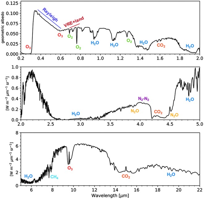
A synthetic UVOIR Earth radiance spectrum at quadrature phase (half illumination). The top panel (0.2 μm < λ < 2.0 μm) is shown in terms of geometric albedo, while the bottom two panels (2 μm < λ < 5 μm; 5 μm < λ < 22 μm) are presented in spectral radiance units (W · m−2·μm−1·sr−1). This spectrum was generated by the VPL 3D spectral Earth model (Robinson et al., 2011; Schwieterman et al., 2015b). Strong absorption features from O2, O3, H2O, CO2, N2O, and CH4 are labeled, in addition to Rayleigh scattering and the location of the VRE. 3D, three-dimensional; CH4, methane; N2O, nitrous oxide; UVOIR, ultraviolet-optical-infrared; VPL, Virtual Planetary Laboratory; VRE, vegetation red edge.
Data–model comparisons have the capacity to validate the detectability of biosignature features through forward modeling (e.g., Des Marais et al., 2002), providing these signatures exist on the modern Earth and their presence is in some way imprinted onto our planet's spectrum. Once validated, those same models can then be altered to simulate planetary spectra for different viewing geometries, cloud conditions, and alternative atmospheric compositions and surface features—in other words, for a wide array of planetary conditions. Through this approach, we can surmise the detectability of biosignatures, including biosignatures proposed for planets such as early Earth (Section 3.4), planets orbiting different stars, or biospheres under different environmental conditions. Sections 4, 5, and 6 describe in more detail studies of individual gaseous, surface, and temporal biosignatures, respectively, many of which use Earth model validations to confirm that spectral models can accurately represent the impact of a proposed biosignature on a planetary spectrum.
3.3. Photochemical studies of terrestrial atmospheres
Photochemical models simulate the interaction of a host star's radiation with a planetary atmosphere. These models use an abbreviated selection of chemical species and reactions to approximate the chemical composition of planetary atmospheres, which may then serve as input for spectral models. The list of species can include both gas-phase and aerosol-phase molecules. These models also track radiative transfer through the atmosphere, focusing on the UV to visible part of the spectrum, as photons in that wavelength range drive most photolysis reactions.
Generally, photochemical models calculate the rate of each reaction in the model (including but not limited to photolysis reactions) as well as physical mixing between model grid points and depositional mass fluxes. This combination allows the creation of a set of equations for the production and loss of each species in each layer of the model atmosphere. Together, these equations define a set of coupled differential equations that are passed to a numerical solver used to find a self-consistent solution for the atmospheric state based on the list of chemical species, their reactions, the stellar irradiation, and the assumed boundary conditions for the model grid.
The main boundary conditions for these models are as follows: (1) the mass fluxes into or out of the atmosphere (usually into the atmosphere at the surface–atmosphere interface, along with a limited flow of light species such as H out of the top of the atmosphere) and (2) the spectral energy flux into the top of the atmosphere, according to the star and the star–planet separation. These boundary conditions can fundamentally alter the composition of the atmosphere. Depending on the purpose and complexity of the photochemical model, it may ultimately calculate a steady-state atmospheric composition that is stable over geological timescales. Alternatively, some photochemical modeling efforts have focused on characterizing the atmospheric consequences of short-duration events, such as stellar flares, by using the same numerical tools.
There are several well-established photochemical models developed by different research groups over the last few decades. The model of the Kasting group (e.g., Kasting, 1982, 1997; Pavlov and Kasting, 2002; Domagal-Goldman et al., 2011) and versions developed therefrom (e.g., Segura et al., 2003, 2007, 2010; Rauer et al., 2011; Arney et al., 2016), the Caltech/JPL model (e.g., Allen et al., 1981; Nair et al., 1994; Yung et al., 1988; Gao et al., 2015), and the Hu group model (Hu et al., 2012, 2013; Hu and Seager, 2014) all share the same general approach to simulating photochemistry. As mentioned earlier, these models include atmospheric chemical reaction lists for the major and minor species and represent a set of partial differential equations governing the concentrations of those species. The models use these equations to evolve gas concentrations toward steady state. Boundary conditions, as mentioned previously, include the impact of planetary processes (e.g., volcanism) on the atmosphere.
Photochemical models have been used in a variety of contexts. They have a long history of modern Earth applications, from modeling the O3 hole and the evolution of greenhouse gas concentrations, to understanding the fate of trace pollutants. In planetary science, these models are often used to interpret data from spacecraft observations, or to simulate data returns from future missions. They also have been used to help understand the atmospheres of early Earth and early Mars by delineating atmospheric states that are consistent with geological and geochemical data.
For exoplanets, photochemical models have been used to simulate potential chemical compositions of a wide variety of worlds, to either interpret observed transit spectroscopy data or to simulate future spectral data, including spectral biosignatures. If spectral simulations are desired, the outputs of a photochemical model are used as inputs to a more detailed radiative transfer model that generates the spectrum. Photochemical models are especially useful for helping understand the contextual information required to interpret a biosignature. Examples of such studies include investigations of the potential atmospheric composition of the Archean Earth (Kasting, 2001; Kharecha et al., 2005; Kaltenegger et al., 2007), of planets orbiting M dwarf stars that have low UV flux (e.g., Segura et al., 2005), of possible by-products of biogenic gases that could serve as biosignatures (e.g., Domagal-Goldman et al., 2011), and of the possibility of false positives from abiotic generation of biosignature gases in alternative planetary environments (see Section 4).
Caution should be taken when interpreting the results of a photochemical model that simulates an atmosphere without the aid of observational constraints. These simulations represent a plausible and sustainable atmospheric state, not necessarily its current chemical composition. A planet could have multiple stable states, given a single set of boundary conditions. Conversely, it is possible for different sets of boundary conditions to reproduce the same stable state. Changing the boundary conditions in the model may result in different sets of possible states. These plausible photochemical model solutions are useful for assessing which of these states may contain detectable biosignatures, as well as to motivate research to constrain better the modeled processes. A prime example is in ongoing research to explain the suite of Earth's different geochemical states through time.
3.4. Earth through time
Life and environment have coevolved on Earth for billions of years. The most significant biologically mediated change was the oxygenation of Earth's atmosphere due to the evolution of oxygenic photosynthesis (OP); in turn, high levels of O2 at Earth's surface eventually allowed the emergence and proliferation of complex, animal life. Evidence for atmospheric O2 first appeared in the rock record ∼2.3 billion years ago (Gyr; e.g., Luo et al., 2016) during a relatively short interval of time referred to as the “Great Oxidation Event” (GOE) (e.g., Holland, 2002) (Fig. 5). Another series of shifts in atmospheric O2 occurred during the late Proterozoic and the early Phanerozoic (∼750 to 460 million years ago). Each geological eon comprises a suite of differences not only in the oxidation state of the atmosphere but also in the composition of the biosphere. Thus, each provides a potential template/analogue for the spectral character of a biogeochemical state of a rocky terrestrial planet in the HZ of its star.
FIG. 5.

Evolution of Earth's atmospheric O2 content through time. Shaded boxes show approximate ranges based on the latest geochemical proxy records, while the curve shows one possible evolutionary trend over time. After Reinhard et al. (2017); see also Lyons et al. (2014).
Nuanced interpretation of potential observations of “Alternative Earth” analogues must also consider the uncertainty and possible lack of detectability of the life-forms that may be only just emerging or that abound but in ways that insufficiently impact the atmosphere. For example, the date of the earliest emergence of O2-evolving photosynthetic cyanobacteria is highly uncertain. O2 may have been produced by cyanobacteria in the late Archean, but at a rate that could not yet produce a strong atmospheric signal (Lyons et al., 2014); indeed, before the GOE, atmospheric “whiffs” of O2, and localized O2 oases in the shallow ocean are inferred from the trace element and isotope records (Planavsky et al., 2014a). Such traces of life would likely elude detection. (The mechanisms for O2 buildup and further details surrounding the trajectory of the O2 content of Earth's atmosphere are described in Section 4.2.1.)
Various modeling studies have attempted to model Earth's atmospheric composition and spectral signatures and their variation over time self-consistently by using coupled photochemical/radiative–convective models and prescribed surface fluxes of various gases or prescribed surface spectral albedos. Relevant examples include models exploring different geologic eons on Earth (Meadows, 2006; Kaltenegger et al., 2007); an early Earth with photosynthetic microbial mats on land (Sanromá et al., 2013), a purple Archean ocean due to photosynthetic purple bacteria (Sanromá et al., 2014); an orange Archean Earth due to an organic-rich atmospheric haze (Arney et al., 2016); and trajectories of O2 fluxes over geologic time given estimated atmospheric concentrations (Gebauer et al., 2017). Such approaches have also been applied to planets orbiting other stars: for example, biosignature gas concentrations and detectability under the UV environments of planets orbiting M stars (Segura et al., 2005; Rugheimer et al., 2015a, 2015b); and organic hazes on Earth-like planets around different stellar types (Arney et al., 2017). The sections that follow describe these biosignature examples and others in detail, with many investigations in the context of photochemical models of alternative planetary scenarios.
4. Gaseous Biosignatures
Gaseous biosignatures can result from direct biological production or from environmental processing of biogenic products leading to secondary compounds. The example treated in detail in the companion article by Meadows et al. (2018) is O2 produced from photosynthesis, and O3 subsequently formed by photochemical reactions involving O2 in the stratosphere. Not all biogenic gases are uniquely biological, and their identification as signs of life will depend strongly on their environmental context. Below we describe biogenic gases known to date, the contexts in which they may or may not be identified as biosignatures, their spectral absorbance features, and how they may be observed.
4.1. Gaseous biosignature overview
To be spectrally detectable, gases in the atmosphere must interact with photons through dissociation, electronic, or vibrorotational transitions. Because many gases absorb near the same wavelengths, it is essential to have the spectral range and/or resolution to discriminate between gases to uniquely identify their presence or absence in an exoplanet atmosphere. Figure 6 shows the line absorption intensities or absorption cross sections for the biosignature gases presented in this section for reference, drawing from the HITRAN 2012 (Rothman et al., 2013) and PNNL (Sharpe et al., 2004) spectral databases. These gases include O2, O3, nitrous oxide (N2O), CH4, methyl chloride (CH3Cl), ethane (C2H6), NH3, dimethyl sulfide (DMS), dimethyl disulfide (DMDS), and methanethiol (CH3SH) (also see reference Tables 3 and 4 in Catling et al., 2018, a companion article in this journal issue).
FIG. 6.

Biosignature gas absorption features. Line intensities (cm−1/[molecule cm−2]) for O2, O3, N2O, CH4, CH3Cl, C2H6, and NH3 are sourced from HITRAN 2012 (Rothman et al., 2013), while cross sections (cm2) for DMS, DMDS, and CH3SH are sourced from the PNNL spectral database (Sharpe et al., 2004). C2H6, ethane; CH3Cl, methyl chloride; CH3SH, methanethiol; DMDS, dimethyl disulfide; DMS, dimethyl sulfide.
4.2. Earth-like atmospheres
An “Earth-like” atmosphere is defined here as one dominated by N2, CO2, and H2O (O2 may or may not be a significant component). An “Earth-like” atmosphere is, by definition, associated with habitability and characterized by the presence of high-molecular-weight gases (μM >> 2) that include a condensable greenhouse gas (H2O), a noncondensable greenhouse gas (CO2), and a noncondensable background gas (N2). This definition is traditionally used to define the circumstellar HZ with 1D radiative–convective climate models (Kopparapu et al., 2013). Earth's atmospheric composition has evolved greatly through time (section 3.4), and so, it is important not to limit the definition of “Earth-like” to atmospheres identical to Earth's modern atmosphere, which represents just a small part of Earth history (e.g., Lyons et al., 2014). Furthermore, an Earth-like atmosphere is not the only type of “habitable” atmosphere conceivable for a rocky, terrestrial planet. Alternative possibilities, such as an H2-dominated atmosphere, are described in Section 4.4.
Each subsection below describes a biosignature gas that has been considered for Earth-like atmospheres (high molecular weight, N2-CO2-H2O dominated). First, the major biological production and buildup mechanisms for the gas are described. Second, abiotic sources are presented and discussed if known. If the buildup of the gas has been studied as a function of the host star spectral type, this is also discussed. Each subsection concludes with a description of the major absorption bands of each gas, and whether they overlap with those from other gaseous biosignatures.
4.2.1. Oxygen (O2)
Molecular O2 and its photochemical by-product O3 have been the most highly referenced astronomical biosignature gases since surveys of nearby habitable planets have been contemplated (e.g., Owen, 1980; Leger et al., 1993; Sagan et al., 1993; Des Marais et al., 2002). This is largely because O2 is a dominant gas in Earth's modern atmosphere (pO2 = 0.21), produces potentially detectable spectral signatures, and is effectively entirely sourced from photosynthesis on Earth. Oxygenic photosynthesis (OP) uses light energy to (indirectly) split H2O, which serves as an electron donor to produce organic matter from CO2, generating O2 as a waste product (Leslie, 2009). The net reaction is often written as follows:
 |
where (CH2O)org represents organic matter and hν is the energy of the photon(s) (where h is Planck's constant and ν is the frequency of the photon). Although the net equation may cancel an H2O from both sides, this representation explicitly shows that the O2 atoms for the evolved O2 (denoted with superscript w) come from the water molecules and not the carbon dioxide. OP makes use of some of the most widely available molecules in the ocean–atmosphere system (H2O and CO2) and harnesses abundant photons from the Sun. It is regarded as perhaps the most potentially productive metabolism on any planet orbiting a star due to the wide availability of its basic substrate and energy source (Kiang et al., 2007a, 2007b). The range of organisms that use OP on our own planet includes plants, algae, and cyanobacteria. It is important to note that oxygenation of an atmosphere is a more complex process than simple production of O2 by photosynthetic organisms. The net photosynthetic reaction given above is, in a general sense, reversible, depleting O2 with the decay of organic matter via aerobic respiration (CH2O + O2 → CO2 + H2O). Photosynthesis produces no net O2 unless some of the organic matter is preserved and ultimately sequestered from the atmosphere. This process is primarily facilitated by burial of organic matter in marine sediments or soils (Berner and Canfield, 1989; Bergman, 2004; Catling, 2014), and is also greatly augmented by burial of sulfide generated by anaerobic sulfate reducers that oxidize organic matter (Berner and Raiswell, 1983). The accumulation of O2 in the atmosphere further requires that the rate of these burial processes is greater than the rate of O2 losses, such as by reactions with reduced volcanic gases (Catling, 2014).
The history of Earth's O2 levels has many nuances, but there is a broad consensus on the major phases (e.g., Lyons et al., 2014). In the Archean eon (4.0–2.5 Ga), O2 levels were very low (pO2 < 10−7), while CH4 levels were believed to be elevated (100–1000 ppm). The GOE occurred ca. 2.4 Ga, near the beginning of the Proterozoic eon, and marked a significant change in the chemistry of the atmosphere, increasing pO2 by several orders of magnitude and decreasing the prevalence of reduced gases such as CH4. After the GOE pO2 rose to as high as 1–10% of modern levels (Kump, 2008), although recent evidence suggests pO2 remained low relative to modern levels for most of the Proterozoic eon (pO2 < 0.1%) (Planavsky et al., 2014b), it was only after a second series of O2 shifts during the late Proterozoic (∼800 million years ago, Ma) and the Paleozoic (∼420 Ma) when pO2 approached modern levels. The late Proterozoic shift occurred roughly contemporaneously with the rise and diversification of complex animal life (Reinhard et al., 2016). Importantly, the initial rise of O2 levels on Earth was delayed until well after the evolution of OP, which had likely occurred by 3.0 Ga (Buick, 2008; Planavsky et al., 2014a)—if not earlier. In any case, understanding the protracted rise of O2 in Earth's atmosphere is an active area of investigation, with critical implications for biosignature evolution on extrasolar planets.
Molecular O2 has a few strong bands in the VIS/NIR region, including the O2-A band (0.76 μm), the O2-B band (0.69 μm), and the O2-g band (0.63 μm). In addition, O2 collisionally induced absorption (O2-O2) occurs at 1.06 μm, and the 1.27 μm O2 band includes contributions both from monomer O2 (a1Δg band) and dimer O2-O2 collisional absorption. At very high O2 concentrations, O2-O2 CIA (also referred to as O4) absorption occurs at 0.445, 0.475, 0.53, 0.57, and 0.63 μm (Hermans et al., 1999; Richard et al., 2012; Schwieterman et al., 2016). In the MIR, O2 has an absorption band at 6.4 μm, but this band is weak and overlaps with much stronger H2O absorption, so is unlikely to be observable at low resolution for habitable planets. In the UV, O2 has strong absorption from photodissociation at wavelengths shorter than 0.2 μm, although this is also true for several other gases, such as CO2. Of these, the O2-A band (0.76 μm) is by far the most preferable target band for direct imaging (reflected light observations) due to its relative strength and the lack of overlap with features from other common gases.
On Earth, the production of abiotic O2 from the photolysis of other O-bearing molecules occurs at a very slow rate. This O2 would not build up to appreciable levels due to the distribution of UV energy from the Sun (which controls the rate of O2 production from O-bearing species such as CO2 and its destruction rate) and geochemical sinks for O2 (e.g., Domagal-Goldman et al., 2014; Harman et al., 2015). However, several scenarios have been described that could allow for the buildup of abiotic O2 for planets orbiting other types of stars. Potential “false positives” for abiotic O2 are reviewed briefly in Section 4.3 and more extensively in Meadows (2017) and Meadows et al. (2018).
4.2.2. Ozone (O3)
The O3 in Earth's stratosphere is the result of photochemical reactions that split O2. The detection of significant O3 in a planetary atmosphere has been proposed as a proxy for photosynthetically generated O2 (Léger et al., 1993, 2011; Des Marais et al., 2002), with the advantage that O3 absorbs strongly in complementary wavelength bands to O2 (e.g., in the UV and MIR). The formation and destruction cycle of O3 is described by the Chapman scheme (Chapman, 1930):
 |
 |
 |
 |
where λ is the minimum wavelength for photodissociation of the given molecule and M is any molecule that can carry away excess vibrational energy (e.g., N2). The O3 layer on Earth reaches peak concentrations of up to 10 ppm in the stratosphere between 15 and 30 km in altitude, but both the value and altitude of the peak O3 concentration vary spatially. The incident UV photon flux and spectrum impact the rate of O3 production and destruction, thus affecting the predicted O3 concentration and profile for planets orbiting different stars even if the planetary O2 abundance is the same (Segura et al., 2003; Rugheimer et al., 2013; Grenfell et al., 2014). Indeed, planets with the same O2 abundances, orbiting the same star, but at different distances, will have slightly different O3 profiles mainly due to differences in UV and temperature structure (Grenfell et al., 2007). Furthermore, particle fluxes from flares around active stars have the capacity to strongly attenuate the predicted O3 column, depending on the strength and frequency of the flare events (Segura et al., 2010; Tabataba-Vakili et al., 2016). Like O2, O3 may be produced through abiotic photochemical mechanisms, with current literature studies indicating that abiotic production is favored most around M dwarf and F dwarf stars (Domagal-Goldman et al., 2014; Harman et al., 2015). This relationship is further discussed in Section 4.4.
O3 possesses absorption features in the UV-VIS-NIR-MIR regions of the spectrum. In the UV, the Hartley–Huggins bands are centered at 0.25 μm and extend from 0.35 to 0.15 μm. These bands are saturated in Earth's spectrum, but caution is warranted since other molecules such as sulfur dioxide (SO2) also absorb in this wavelength region (Robinson et al., 2014). In the visible, the Chappuis bands extend from 0.5 to 0.7 μm and contribute to the “U” shape of Earth's overall UV-VIS-NIR spectrum, a feature that distinguishes Earth's color from those of other planets at even very low (Δλ ∼0.1 μm) spectral resolution (Krissansen-Totton et al., 2016b). O3 has several weak bands in the NIR at 2.05, 2.15, 2.5, 3.3, 3.6, 4.6, and 4.8 μm. Those at the longer wavelengths are the strongest, although many of these bands overlap with absorption features from H2O and CO2. In reflected light, the UV band is the strongest feature from O3. O3 also imprints strong features on the emitted, thermal infrared portion of Earth's spectrum. The strongest and most well studied of these is the 9.65 μm band, which occurs in the middle of Earth's thermal infrared spectral window (Des Marais et al., 2002). The 9.65 μm band would be a prime target for an infrared-capable telescope, such as the previously envisioned Terrestrial Planet Finder–Infrared mission (TPF-I) (Beichman et al., 2006; Lawson et al., 2006; Traub et al., 2007) or its ESA equivalent Darwin (Cockell et al., 2009b). Caution should be given to the overlap from the “doubly hot” band of CO2 at 9.4 μm, which would also produce absorption at 10.5 μm (Segura et al., 2007, see their Fig. 5b). In addition, other gases, including CH3Cl, DMS, DMDS, and CH3SH, have overlapping absorption features near the 9.65 μm band (Pilcher, 2003, see sections 4.2.5 and 4.2.6 below). Therefore, it is essential to obtain spectral information at other wavelengths to confidently detect O3. Finally, there is a weak O3 band at 14.08 μm, which is completely swamped by the 15 μm CO2 band. To summarize, the best prospects for detecting O3 are the Hartley–Huggins bands centered at 0.25 μm in the UV, the subtler Chappuis band extending from 0.5 to 0.7 μm in the visible, and the 9.65 μm band in the MIR.
4.2.3. Methane (CH4)
Methanogenesis is an ancient form of anaerobic microbial metabolism that produces CH4 as a waste product, most commonly by either respiring CO2 as a terminal electron acceptor or disproportionating acetate to CH4 and CO2. These reactions can be written as follows:
 |
 |
where H2 is hydrogen gas and CH3COOH is acetic acid—a decay product from fermentation of organic matter. On Earth, the single-celled organisms responsible for methanogenesis, called “methanogens,” are restricted to the domain Archaea. Methanogenesis is the dominant source of nonanthropogenic CH4 in Earth's modern atmosphere, and CH4 has consequently been suggested as a potential biosignature on Earth (e.g., Sagan et al., 1993) and on Mars (e.g., Krasnopolsky et al., 2004). However, there are many potential abiotic CH4 sources, almost all of which involve water–rock reactions. See Etiope and Sherwood-Lollar (2013) for a review of abiotic CH4 sources on Earth.
Primitive planet-building material from the outer Solar system, beyond the ice line, is replete with CH4, since it is the most thermodynamically stable form of carbon in reducing (i.e., H-abundant) conditions. Therefore, planetary bodies constructed from this material may be expected to contain an abundance of abiotic CH4. Such is the case in the atmosphere of Saturn's icy moon Titan, whose atmosphere contains 5% CH4 by volume. CH4 is likewise the most thermodynamically stable form of carbon in highly reducing, H2-dominated atmospheres. Therefore, CH4 is often viewed as a companion biosignature that would be most compelling if observed together with O2/O3 or other strongly oxidizing gases. CH4 may also serve as a biosignature or habitability marker with the presence of CO2, since the presence of CO2 implies the atmosphere's redox state is more oxidizing and thus not conducive to producing CH4 as the most stable form of carbon (Titan's atmosphere has very little CO2). In an atmosphere with a significant amount of CO2, the CH4 would have had to originate from biology or from abiotic water–rock reactions, an indirect evidence of liquid water in the planetary environment.
The dominant sinks for CH4 in the modern Earth's atmosphere involve oxidation of CH4 by radical species, such as hydroxyl (OH), O(1D), or Cl, for example:
 |
 |
Formaldehyde (H2CO) formed through this reaction can be further oxidized to CO2 and H2O, or incorporated into rain and transported to the ocean. In more reducing atmospheres, CH4 photodissociation can drive the formation of longer chain hydrocarbons, ultimately leading to organic haze particles, as observed in Titan's atmosphere. Under anoxic conditions, CH4 tends to be long lived in the atmosphere, but the advent of OP on Earth eventually led to the dramatic reduction of atmospheric CH4 content (Pavlov and Kasting, 2002).
CH4 absorbs throughout the VIS-NIR-MIR with its strongest bands at 1.65, 2.4, 3.3, and 7–8 μm. There are also weaker bands at (in order of increasing strength) 0.6, 0.7, 0.8, 0.9, 1.0, 1.1, and 1.4 μm. However, CH4 bands in the visible and NIR are relatively weak at the abundances of modern Earth. The strongest band in the infrared, centered between ∼7 and 8 μm, absorbs at the long-wavelength wing of the ∼6 μm H2O band and overlaps with N2O, which also absorbs strongly between 7 and 9 μm. At each of CH4's strong bands, it overlaps with H2O absorption, which makes uniquely detecting CH4 problematic at low spectral resolution.
4.2.4. Nitrous oxide (N2O)
N2O is produced by Earth's biosphere via incomplete denitrification of nitrate (NO3−) to N2 gas. A simplified scheme for denitrification can be written as follows:
 |
N2O has been proposed as a strong biosignature, in part, because its abiotic sources are small on modern Earth and because it has potentially detectable spectral features (Sagan et al., 1993; Segura et al., 2005; Rauer et al., 2011; Rugheimer et al., 2013, 2015a). The preindustrial concentration of N2O in Earth's atmosphere was ∼270 ppb (Myhre et al., 2013). It has been proposed that euxinic oceans (replete with hydrogen sulfide [H2S]) during portions of the Proterozoic epoch would have stifled the bioavailability of copper that facilitates the last step in the denitrification process (i.e., the reduction of N2O to N2), allowing biogenic N2O to build up in the atmosphere with possible climatic implications (Buick, 2007; Roberson et al., 2011). For a biogeochemically analogous world, N2O may exist at higher concentrations than seen on modern Earth (e.g., Meadows, 2006; Kaltenegger et al., 2007). Photochemical modeling of terrestrial atmospheres around M dwarf stars has shown that N2O would build up to higher concentrations than on an Earth–Sun analogue given the same source fluxes (Segura et al., 2005; Rauer et al., 2011; Rugheimer et al., 2015a). This is a mechanism like that described for CH4 above (Section 4.2.3) and is due, in large part, to a paucity of near-UV photons from cool M stars owing to their lower effective temperatures.
A small abiotic source of N2O on Earth is known from “chemodenitrification” of dissolved nitrates in hypersaline ponds in Antarctica (Samarkin et al., 2010), although the synthesis of NO3− requires photosynthetically generated O2. In this scenario, therefore, abiotic N2O production is ultimately an expression of biological activity on Earth. A small amount of N2O is also produced by lightning (Levine et al., 1979), although the estimated contribution of total atmospheric N2O from lightning on Earth is 0.002% (Schumann and Huntrieser, 2007). Around young or more magnetically active stars, N2O may build up abiotically due to enhanced production of NO and NH from extreme ultraviolet (EUV-XUV) and particle flux-induced photodissociation and ionization, driving the reaction NO + NH →N2O + H (Airapetian et al., 2016). However, abiotic processes that generate N2O create associated nitrogen oxide (NOx) products in far greater abundance than N2O (Schumann and Huntrieser, 2007), some of which may be spectrally observable and thus provide a signature of this process. In contrast, cosmic ray events are predicted to destroy N2O and favor production of nitric acid (HNO3) (Tabataba-Vakili et al., 2016).
Ultimately, the confidence with which N2O can be considered a robust biosignature must be evaluated in the context of the stellar environment as well as through observation of other photolytic products that would indicate abiotic N2 oxidation. Fortunately, current studies suggest that abiotic sources of N2O are small except in cases where its production would be contextually predictable or inferable from planetary observations at many wavelengths, although disentangling N2O spectral features from overlapping gases may be difficult at low to moderate spectral resolving powers. N2O has significant bands centered at 3.7, 4.5, 7.8, 8.6, and 17 μm, with several weak bands between 1.3 and 4.2 μm and between 9.5 and 10.7 μm. However, most of these bands are weak at Earth-like abundances and/or overlap with other potentially abundance gases such as H2O, CO2, or CH4, which may make detecting N2O challenging (Fig. 4). Observations at very high spectral resolution powers, at the level required to identify individual lines, may allow unique detection of N2O from overlapping gas absorption features.
4.2.5. Sulfur gases (DMS, DMDS, CH3SH) and relation to detectable C2H6
Biology produces several sulfur-bearing gases as direct or indirect products of metabolism. The direct products of metabolism tend to be simple sulfur gases such as H2S, carbon disulfide (CS2), carbonyl sulfide (OCS), and SO2, although these are also produced in abundance by abiotic volcanic and hydrothermal processes and thus are not strong biosignature gas candidates [e.g., see Arney et al. (2014), for an analysis of these gases in the Venusian atmosphere]. More complex sulfur gases such as CH3SCH3 or DMS, CH3S2CH3 or DMDS, and CH3SH (also known as methyl mercaptan) are produced as indirect products of metabolism but have few if any known abiotic sources on modern Earth.
The organosulfur gases (CH3SH, DMS, DMDS) are produced by bacteria and higher order life-forms in a variety of environments, including wetlands, inland soils, coastal ecosystems, and oceanic environments (Rasmussen, 1974; Aneja and Cooper, 1989). There are two principal routes to the production of DMS. The first is the biological degradation of the compound dimethylsulfoniopropionate (DMSP), which is found primarily in eukaryotic organisms such as certain types of marine algae (Stefels et al., 2007). This pathway is believed to be the dominant source of DMS, which is the largest source of organosulfur gas in the modern atmosphere (Stefels et al., 2007). Second, DMS (and DMDS) can ultimately result from the production of CH3SH, itself a decomposition product of the essential amino acid methionine. Microbial mats containing cyanobacteria and anoxygenic phototrophs produce measurable amounts of CH3SH, DMS, and DMDS (Visscher et al., 1991, 2003), likely from the reaction of short-chain organic compounds produced by the phototrophs reacting with sulfide produced by sulfate-reducing bacteria.
It has been hypothesized that the more reducing environment of early Earth would have been conducive to the production of greater volumes of sulfur gases by the anoxic biosphere (Pilcher, 2003; Domagal-Goldman et al., 2011). The potential for photochemical buildup and the detectability of sulfur gases on early Earth exoplanet analogues were investigated by Domagal-Goldman et al. (2011), who considered biospheres that produced between 1 and 30 times the estimated modern-day fluxes for these gases during the Archean eon. These authors found that DMS, DMDS, and CH3SH were rapidly destroyed by photolysis reactions in the atmosphere, leading to near-zero mixing ratios at all but the lowest levels of the atmosphere (e.g., see Domagal-Goldman et al., 2011; their Fig. 2). Moreover, that study found that, even for biospheres with very high sulfur fluxes, their low abundance in the atmosphere, a consequence of efficient photochemical destruction, would render DMS, DMDS, and CH3SH spectrally undetectable except in the narrow case of an M star with suppressed UV activity (Domagal-Goldman et al., 2011). However, the study also found that the cleaving of methyl (CH3) radicals from DMS and DMDS by UV radiation catalyzed the photochemical buildup of C2H6 far beyond the level expected for the abundance of CH4 in the atmosphere, which is otherwise the primary precursor to C2H6. Consequently, it was proposed that this anomalously high C2H6 signature would be suggestive of a sulfur biosphere (Domagal-Goldman et al., 2011), although this may only be the case for high flux rates of organosulfur gases in combination with stellar hosts with a favorable UV spectrum for C2H6 production.
However, the detection of C2H6 alone would be an ambiguous signature, since photochemical processing of other carbon-bearing species such as CH4 can generate it. The link to an organosulfur biosphere would necessitate constraints on the C2H6 to CH4 abundance ratio to determine whether there is an overabundance of C2H6 relative to that which would be expected only from photochemical equilibrium with the retrieved CH4 abundance. This would reveal the likelihood of other sources of CH3 such as DMS that would act to increase the amount of C2H6. Necessarily, this comparison would also require forward modeling of the atmospheric photochemistry given the UV spectrum of the host star, the retrieved CH4 abundance, other measured or likely atmospheric constituents, and additional planetary parameters such as the atmospheric temperature structure, which may or may not be available.
Although Domagal-Goldman et al. (2011) evaluated only synthetic direct-imaging spectra in their investigation of DMS and DMDS spectral detectability, their results also apply to transmission spectroscopy. Although transmission spectroscopy can enhance the signature of gases with low abundances through path length effects (e.g., Fortney, 2005), this advantage is relevant only for gases with a presence in the portions of the atmosphere probed by transmission spectroscopy. Due to the combined effects of refraction, clouds, and aerosols, the lowest levels of an Earth-like atmosphere are not accessible (García Muñoz et al., 2012; Bétrémieux and Kaltenegger, 2014; Misra et al., 2014a, 2014b). Domagal-Goldman et al. (2011) found DMS and DMDS drop to near-zero abundance at all but the lowest levels of the atmosphere. Combined with results from direct imaging, these relationships suggest DMS and DMDS are examples of gases that, while exhibiting measurable spectral signatures in a laboratory setting, may never reach the required abundances to be directly detectable over interstellar distances for plausible biospheres. More encouragingly, their presence may be indirectly inferred by the detection of their photochemical by-products, in this case C2H6. This approach is analogous to the detection of O3 to infer the presence of its primary precursor, O2, in the atmosphere, with appropriate caveats considering other photochemical sources of C2H6 stated previously.
The strongest features of DMS are in the MIR at 6–7, ∼10, and ∼15 μm. DMDS absorbs strongest spectrally in the MIR at 7, 8–9, and 17 μm. CH3SH has its strongest features at 6–7, 8–12, and 14–15 μm. Notably, these gases all have absorption features that overlap with the 9.65-μm O3 band (Pilcher, 2003), which could be problematic at low spectral resolution. C2H6 has strong spectral signatures at 6–7 and 11–13 μm and a weaker band at 3.3 μm.
4.2.6. Methyl chloride (CH3Cl)
CH3Cl, or chloromethane, is a biogenic gas whose major sources on Earth are both natural and anthropogenic: algae in the oceans (Singh et al., 1983; Khalil and Rasmussen, 1999), tropical/subtropical plants (Yokouchi et al., 2002, 2007; Saito and Yokouchi, 2006), aquatic plants in salt marshes (Rhew et al., 2003), terrestrial plants (Saini et al., 1995; Rhew et al., 2014), fungi (Harper, 1985; Watling and Harper, 1998), decay of organic matter (Keppler et al., 2000; Hamilton et al., 2003), biomass burning (Lobert et al., 1999), and industrial processes involving organic matter (Kohn et al., 2014; Thornton et al., 2016). Volcanoes may be an abiotic source (Schwandner et al., 2004; Frische et al., 2006). The relative contributions of these biological and abiotic sources remain unknown for the modern and ancient Earth (Keene et al., 1999). The biological production mechanisms for CH3Cl are also poorly characterized (Rhew et al., 2014), although a CH3 chloride transferase enzyme has been identified (Ni and Hager, 1998), and methylation of plant pectin (during degradation) is a general pathway across taxa (Hamilton et al., 2003). It appears there is not a unique pathway to production, but biosynthesis in numerous organisms, decay or combustion of organic matter, and volcanic gas-phase reactions can all produce CH3Cl.
Spectral absorbance features occur at 3.3, 7, 9.7, and 13.7 μm (Rothman et al., 2013) (note overlap with the 9.65 μm O3 band). The dominant pathway for removal of CH3Cl is reaction with OH radical, with an estimated atmospheric lifetime of 1.3 years on Earth (WMO, 2003). In stellar environments with extremely low NUV flux suppressing OH formation, such as would take place in the quietest theoretical lower limit of M dwarf activity with no chromospheric excess UV flux, there is a potential to build up CH3Cl to detectable levels (Segura et al., 2005), although the feature overlaps with other expected features such as H2O, CO2, O3, and CH4. CH3Cl would be best observed at 13.7 μm in the wings of the CO2 feature (Rugheimer et al., 2015a).
4.2.7. Haze as a biosignature
Geochemical evidence suggests the existence of an intermittent organic haze during the late Archean geological eon (Zerkle et al., 2012; Izon et al., 2017). This haze would have dramatically impacted Earth's climate, photochemistry, and spectral observables. The putative Archean organic haze is like the organic haze in Titan's atmosphere in that it likely forms from CH4 photochemistry. At the CO2 levels suggested for the Archean Earth (atmospheric fractions of roughly 10−3–10−2) (Driese et al., 2011), a ratio of CH4/CO2 of about 0.2 is required to initiate the formation of a thick organic haze (e.g., Trainer et al., 2006). CH4 on Earth can be produced by both abiotic and geological processes. On the modern Earth, biological processes produce the bulk of the atmosphere's CH4, as was likely during the Archean eon (Kharecha et al., 2005). The dominant abiotic CH4 source on modern Earth—and likely the dominant abiotic source during the Archean—is serpentinization, the hydration of ultramafic minerals such as olivine and pyroxene (Kelley, 2005; Etiope and Sherwood-Lollar, 2013; Guzmán-Marmolejo et al., 2013), although the ultimate source of CH4 in serpentinizing systems is not entirely clear (McDermott et al., 2015; McCollom, 2016).
Coupled photochemical-climate modeling has shown that producing a thick organic haze in the atmosphere of an exoplanet with Archean Earth-like CO2 levels requires surface CH4 flux rates consistent with measured modern biological CH4 production [roughly 1011 molecules/(cm2·s)] and theoretical Archean biological CH4 production rates [∼0.3–2.5 × 10¹¹ molecules/(cm2·s), Kharecha et al., 2005; also see Arney et al., 2016, 2017, 2018]. Like CH4 itself, organic haze would not definitively imply the existence of life, but organic haze produces strong, broadband absorption features at UV-blue wavelengths (the reason why Titan is orange), potentially more detectable than CH4 itself. Because haze dramatically alters the broadband shape of a planet's reflected light spectrum (Fig. 7), it may provide a relatively simple means of flagging interesting targets for follow-up observations to search for other signs of habitability and life. Organic haze formation is incompatible with O2-rich atmospheres and so would exist exclusively on exoplanets with reducing atmospheres, providing a useful means for identifying potentially inhabited worlds with more reducing atmospheres than modern-day Earth.
FIG. 7.
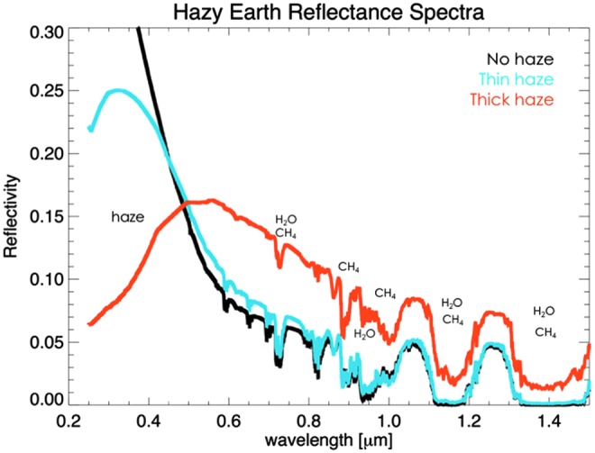
Spectra of Archean Earth with three different haze thicknesses for atmospheres with 2% CO2 (Arney et al., 2016). The haze absorption feature at UV-blue wavelengths is strong and potentially detectable at spectral resolving powers as low as 10. UV, ultraviolet.
In the same way that organic haze could serve as an indicator of the CH4/CO2 ratio, and therefore, a gauge of the CH4 flux, it has been proposed that sulfur aerosols (S8 and H2SO4) could serve as a proxy of the H2S/SO2 ratio and a gauge of the H2S flux (Hu et al., 2013). At high H2S/SO2 flux ratios, and a neutral to reducing atmosphere, S8 aerosols would be formed. At low H2S/SO2 flux ratios, H2SO4 is formed preferentially over S8. Oxidizing conditions that include even trace amounts of O2 (<10−5 present atmospheric level [PAL] pO2) result in H2SO4 formation dominating over S8 (Pavlov and Kasting, 2002; Zahnle et al., 2006). Geologic H2S fluxes can be complemented by biological H2S fluxes originating from microbial sulfur reduction or sulfur disproportionation, common metabolic processes on Earth (Finster, 2008). The spectral properties of S8 and H2SO4 aerosols differ with S8 aerosols absorbing in the UV-blue region, while H2SO4 displays strong absorption at λ > 2.7 μm. In principle, if volcanic H2S and SO2 fluxes could be constrained, sulfur aerosol properties may indicate whether implied H2S fluxes imply an additional, biological source of H2S, serving as a potential biosignature (Hu et al., 2013). However, constraining volcanic sources remotely will be difficult and would require estimating the extent of subaerial versus submarine volcanism, which favors different H2S/SO2 outgassing proportions. More conservatively, characterizing sulfur haze properties would allow an independent assessment of the redox state of the atmosphere with S8 indicating reducing conditions, and H2SO4 indicating oxidizing conditions. This could contribute to the overall appraisal of planetary habitability even if biogenic H2S fluxes were not constrained.
4.2.8. Other gases
The gases described above do not exhaust the list of volatile compounds produced by life on Earth, but encompass the unambiguous biogenic species widely believed to have been able to produce a measurable spectral impact at some point in Earth history. Other biogenic compounds are generated in abundance by Earth's biosphere but are not observed to rise to remotely detectable concentrations in a planetary disk average or are also produced in abundance by common abiotic processes. For example, isoprene is a common volatile organic compound produced by plants, phytoplankton, and animals, including humans (King et al., 2010), but is quickly destroyed photochemically in Earth's oxic atmosphere (Palmer, 2003). Other secondary metabolic products (in contrast to direct products of metabolism such as O2) fit this mold, and are reviewed in Seager et al. (2012; e.g., their Table 3). Gases that are generated as products of metabolic processes, but also have common abiotic sources, encompass almost all simple molecules, including H2S, SO2, N2, H2O, CO2, and many more.
4.3. “False positives” for biotic O2/O3 and possible spectral discriminators
The stated consensus as expressed in Des Marais et al. (2002) was that abiotic O2 could be found on terrestrial exoplanets, but only on planets outside of the HZ (i.e., either too close to the star or too far away to support habitable conditions). A tectonically active, water-rich planet with an active hydrological cycle was thought to have the capacity to remove abiotic O2 from the atmosphere through geochemical or weathering reactions [e.g., the reaction of O2 with reducing volcanic gases or crustal ferric iron, Fe(II)].
The prevailing view has now evolved since Des Marais et al. (2002), with at least a few plausible mechanisms for generating O2 abiotically on planets within the HZ, including from robust photolysis of CO2 or a history of extreme hydrogen escape and O2 buildup (e.g., Domagal-Goldman and Meadows, 2010; Hu et al., 2012; Domagal-Goldman et al., 2014; Tian et al., 2014; Wordsworth and Pierrehumbert, 2014; Gao et al., 2015; Harman et al., 2015; Luger and Barnes, 2015). For example, several authors have found that some abiotic O2 (and O3) could be produced in a prebiotic Earth-like, N2-CO2-H2O atmosphere with a surface ocean if the UV spectrum of the host star favored robust CO2 photolysis (Domagal-Goldman et al., 2014; Tian et al., 2014; Harman et al., 2015). These authors find that the extent of abiotic O2/O3 depends on a host of other boundary conditions (such as the flux of reducing gases and compounds), which may vary greatly from planet to planet. Significant hydrogen escape and O2 buildup may be facilitated by atmospheres with low amounts of noncondensing gases lacking a cold trap (Wordsworth and Pierrehumbert, 2014) or an extended greenhouse phase after planetary formation due to the protracted superluminous premain sequence evolution of M dwarf stars (Luger and Barnes, 2015; Tian, 2015). These O2 buildup scenarios need not completely deplete the entire H2O reservoir of the planet, but may exhaust O2 sinks [such as crustal Fe(II)].
Each of the abiotic processes described above would generate their own spectral fingerprint, such as the simultaneous spectrally detectable presence of CO and O2 from CO2 photolysis (Harman et al., 2015; Schwieterman et al., 2016) or the absence of N2 (Wordsworth and Pierrehumbert, 2014), which may be revealed through a lack of (N2)2 absorption (Schwieterman et al., 2015b) or constraints on atmospheric mass through Rayleigh scattering (e.g., Benneke and Seager, 2012). Highly evolved atmospheres that have experienced significant H-loss could be identified by highly density-dependent O4 features (Schwieterman et al., 2016) and by extended scale heights in transmission spectroscopy in the case of O-enriched He-dominated atmospheres (Hu et al., 2015). Conversely, the existence of plausible mechanisms for abiotic O2 strengthens the case for searching for biosignature couples such as O2 + CH4, possibly establishing more robust evidence for life. Other novel routes for abiotic O2 buildup require highly desiccated atmospheres in tandem with the UV spectral energy distribution found in M dwarf stars (e.g., Gao et al., 2015), which may be identified through the absence of conventional habitability markers such as water vapor.
Considering all the above, our understanding of the plausible abiotic mechanisms for the presence of O2 in exoplanet atmospheres is accompanied by action points that would assist in designing instruments and strategies for observing and characterizing potential biosignatures. This topic is explored extensively in Meadows (2017) and a companion article in this issue, Meadows et al. (2018).
4.4. Biosignatures in other types of atmospheres
It has been shown that atmospheres with H2-dominated compositions could be habitable even with little CO2 and at instellations lower than those predicted for the outer edge of the traditional HZ (Stevenson, 1999; Pierrehumbert and Gaidos, 2011; Seager, 2013). In addition, studies of exoplanet demographics from the Kepler mission have found that the most common type of planet is intermediate in radius (and mass) between Earth and Neptune (Batalha, 2014; although this conclusion is limited by the completeness of the Kepler sample, which is biased toward short-period planets). Referred to as “super-Earths,” the stronger gravity of these planets increases the likelihood that their atmospheres could contain a low-molecular-weight component (i.e., H2, He) over geologic time. (Note this does not suggest super-Earths may have a massive H2 envelope like that of Neptune, which is not supported by data [e.g., Rogers, 2015]; the low-molecular-weight component would have to be small enough, relative to the planet's overall mass, to have a negligible impact on bulk density. This does rule out a significant H2 fraction of a thin, terrestrial atmosphere, which is a negligible portion of a rocky planet's overall mass.)
However, we do not currently have examples of either abiotic or biological scenarios for rocky planets with significant H2 fractions in our Solar System, although both early Mars and early Earth may have had a climatically significant H2 component that requires further study (e.g., Tian et al., 2005; Ramirez et al., 2013; Wordsworth and Pierrehumbert, 2013). This situation introduces additional challenges for establishing biosignatures. However, if robust biosignatures are identified for exoplanets with a substantial component of H2 or He, they will be significantly more detectable in transit spectroscopy because they will increase the scale height and therefore the transmission depths of spectral features (Miller-Ricci et al., 2009; Seager et al., 2013b; Ramirez and Kaltenegger, 2017).
Many reducing, H-bearing gases (e.g., CH4, C2H6, H2S) are problematic biosignatures in these atmospheres because abiotic equilibrium or kinetic processes could efficiently produce them. Just as in high-molecular-weight atmospheres, the most compelling signatures will be those that have equilibrium or kinetic barriers that prevent them from being easily generated abiotically.
Plausible biosignatures in H2-dominated atmospheres could include NH3, CH3Cl, DMS, and N2O (Seager et al., 2013a, 2013b). Seager et al. (2013a, 2013b) proposed that NH3 may be generated biologically in atmospheres dominated by H2 and N2 via the reaction N2 + 3H2 → 2NH3 since it is exothermic (energy yielding). Kinetic barriers prevent this reaction from occurring spontaneously at habitable temperatures. However, false positives include outgassed NH3 from primordial material in the solid planet, exogenous delivery of cometary material, buildup from low UV emission from the host star, and chemical equilibrium reactions if temperature conditions are met in the subsurface or deep in a thick atmosphere. NH3 is thus far the only biosignature candidate unique to H2-dominated atmospheres (Seager et al., 2013a, 2013b). NH3 has major absorption complexes near 2.0, 2.3, 3.0, 5.5–6.5, and 9–13 μm.
DMS, CH3Cl, and N2O are possible biosignature gases for both H2-dominated and Earth-like atmospheres (Seager et al., 2013a, 2013b; Sections 4.2.4 to 4.2.6 and references therein). N2O would be an intriguing biosignature on an H2-dominated world, because it would have no abiotic sources. However, it would not be generated from energy-yielding metabolism (since producing it would be energetically unfavorable in an H2 atmosphere)—although it could be an incidental by-product of metabolism in niche cases.
Additional biosignature gases in novel environmental contexts are currently being explored, but are highly speculative. An alternative, complementary, approach to empirically examining biosignatures gases is instead to begin with “all small molecules” that may be produced by (exo)life and subsequently filter those gases by their potential buildup in an atmosphere and their potential spectral detectability (Seager et al., 2016). Potential future directions in assessing novel biosignature gases are explored more deeply in the Walker et al. (2018) companion article in this issue.
4.5. Effects of the host star spectrum on photochemistry
In studies of planetary atmospheres generated by the fixed supply of gases (e.g., volcanic outgassing at a specified rate), changing the host star's type, and by extension of the wavelength distribution of light impinging on the planet, can dramatically alter the steady-state composition of the atmosphere. As mentioned in Sections 4.2.1–4.2.2 and 4.2.4–4.2.5, changes in the UV environment when transitioning from a G-type to an M-type star lead to increases in the concentrations of some biogenic gases, such as N2O, O3, and DMS (Segura et al., 2005; Rugheimer et al., 2015a). This possibility holds true for other gases as well, such as the abiotic generation of O2 mentioned in Section 4.3. In addition, these changes can be driven by a host star's age, since a star's spectrum changes with time, potentially even before the star has evolved on to the main sequence (e.g., Ramirez and Kaltenegger, 2014; Luger and Barnes, 2015). Finally, the amount of radiation the planet receives represents one part of the equation when determining whether the planet has liquid surface water. Water vapor photolysis drives several catalytic cycles in the modern Earth's atmosphere and is expected to play a similar role in the atmospheres of planets around other stars. Taken together, the host star's spectrum has primary and secondary roles in determining the chemical composition of a planet's atmosphere.
One persistent consequence of the host star's spectrum is the planet's UV environment, as mentioned previously. Because UV photons are responsible for most of the photochemistry occurring in a planet's atmosphere, decreasing amounts of UV can lead to high concentrations of gases otherwise destroyed by UV photolysis, perhaps to unphysical levels if other potential sinks are not accounted for. For example, Zahnle et al. (2008) pointed out that a dense, cold, CO2-dominated early martian atmosphere would be unstable to rapid and irreversible conversion to CO and O2 (a “runaway”). A similar result was found by Gao et al. (2015) for Mars-like planets orbiting M dwarf host stars. In these cases, the cold surface temperatures limited water vapor photolysis, which in turn prevented the efficient catalytic recombination of CO and O2. For the O2 false-positive mechanism outlined in Section 4.3 by Harman et al. (2015), this same process occurs due to a lack of UV photons, rather than a lack of water vapor. On the other end of the spectrum, large amounts of UV radiation, in conjunction with higher stellar luminosities, can drive the photolysis (and ultimately the loss) of water vapor (Luger and Barnes, 2015).
Returning to low-UV environments, each potential biosignature gas mentioned in Sections 4.2.1–4.2.5 is subject to UV photolysis. Because of this, the same sort of “runaway” behavior has been noted for both CH4 and N2O for planets orbiting UV-inactive late M stars (Rugheimer et al., 2015a). These cases persist even with large increases in the UV flux (Rugheimer et al., 2015a), suggesting that, at least for planets orbiting stars that are typically UV-quiet, we might expect higher concentrations of relevant biosignature gases, but as mentioned previously, lower UV fluxes also give rise to false-positive scenarios.
4.6. Impacts of flares and particle events on biosignature gases
In addition to a host star's time-averaged UV irradiation, stars can generate flares, charged particle events, and coronal mass ejections. The strength and frequency of these types of events vary with the star's size and age. For example, the young Sun was likely much more active than it is today, potentially for hundreds of millions of years (Güdel et al., 1997), and smaller stars (M4 and later) tend to be active for even longer periods of time, up to 8 Gyr (West et al., 2008). For terrestrial planets, these events can drive the photochemical modification of the atmosphere away from steady state, and, if strong flares and events occur frequently enough, could result in those modifications becoming the norm. If the planet in question is like prebiotic Earth, this situation could lead to the buildup of N2O from abiotic nitrogen oxidation (Airapetian et al., 2016), which may constitute a false positive. Alternatively, higher XUV fluxes driven by an increased number and intensity in flares may also drive more substantial atmospheric escape, which may render a terrestrial planet uninhabitable—in line with estimates for planets in high time-averaged UV environments (e.g., Luger and Barnes, 2015; Airapetian et al., 2017). In addition, planets around smaller stars may be subject to increased cosmic ray fluxes, which can modify the concentrations of key biosignature gases through the creation of NOx radicals (Grenfell et al., 2012).
Besides potentially producing false positives and desiccating planetary atmospheres, high-energy events can decrease the prevalence of other biosignature gases. An Earth-like planet struck by a single strong stellar flare would see only a small decrease in O3 concentrations initially due to enhanced UV irradiation, but charged particles would produce a much larger decrease occurring over longer timescales, weeks to months (Segura et al., 2010). Subsequent flares within the flare recovery window would be expected to aggravate this effect but may be insufficient to completely remove the O3 layer (Tabataba-Vakili et al., 2016). This flare activity may introduce detectable concentrations of other gases such as HNO3, potentially allowing for the characterization of flaring trends beyond the observational window (Tabataba-Vakili et al., 2016), which provides further motivation for better constraints on the X-ray, UV, and charged particle environment for observed exoplanets.
5. Surface Biosignatures
Life may alter the spectrum of the surface of a planet through a variety of mechanisms, which include absorption and reflection of light by pigments in living organisms, scattering by the physical structures of organisms (including individual organisms and community architectures), degradation products of biological molecules, fluorescence of pigments, and bioluminescence. Each of these mechanisms may produce remotely detectable biosignatures; however, not all such biological spectral phenomena may be widespread enough to be detectable at the global scale on Earth, and not all are without abiotic mimics. Below, we catalog surface biological spectra arising from photosynthesis, other pigments, and reflectance features associated with cellular protection and ecological functions, and chiral biomolecules.
We summarize the spectral properties of known biomolecules on Earth, but note that only one surface spectral signature, the VRE, has been confirmed to produce a unique biological fingerprint on the disk-averaged spectrum of our planet. Other biomolecules that have been suggested in the literature thus far remain subjects for further research. In general, even on Earth, the spectra of such molecules can be subject to variation according to environmental conditions, physiological status, and species differences, tempering the likelihood of attaining diagnostic features that fingerprint exactly the molecules in question as is the case for gaseous absorption spectra. However, “edge” spectra are potentially powerful surface biosignatures that can occur throughout the visible and NIR (Hegde et al., 2015; Schwieterman et al., 2015a; Poch et al., 2017) and whose expression can depend on a host of factors, including intrinsic chemistry of major biomolecules, pigment acclimation relative to the environmental photon flux spectrum, and evolutionary contingencies. While we begin to explore the question of how these signatures may manifest on another planet, Walker et al. (2018) further address the challenges involved and explicitly outline fruitful avenues for future empirical and theoretical studies.
5.1. Photosynthesis
Since the review by Des Marais et al. (2002), OP remains the source of the most robust known planetary-scale biosignature: atmospheric O2 and the surface reflectance spectrum of vegetation, the VRE. Anoxygenic photosynthesis, which likely evolved before the oxygenic variety, produces potentially diagnostic surface features, described below, but no robust gaseous signatures are yet known. Because photosynthesis leverages incident energy from the host star, it is the metabolic process with the greatest potential to affect the planetary environment, and is therefore essential to understand when making predictions of planetary-scale biosignatures. At our current state of understanding, it remains uncertain what different pigment colors might result from photosynthesis under different stellar irradiation and what other biogenic gases might result from photosynthesis adapted to other planets. The precise developmental pathway of photosynthesis, and specifically the evolutionary sequence of OP, is still an active area of inquiry (see Meadows et al., 2018, this issue), and scientific understanding is not yet sufficient to say whether the same or similar route of evolution would be followed on another planet. However, light energy use and storage in photosynthesis obey certain universal principles that also apply for solar energy from photovoltaic cells and must apply as well on exoplanets. The use of light energy to drive the movement of electrons is a remarkable feat of nature, involving a coordination of quantum dynamics and redox chemistry. In lieu of having a complete catalog of specific wavelengths to target for spectral features of surface pigments, understanding the fundamentals of photosynthesis, and the unknowns, should allow us to speculate on alternative expressions of photosynthesis on other planets.
Below we summarize basic principles of photosynthesis as well as important unknowns, the molecular nature and spectral features of light harvesting pigments, and how the VRE results. We then review the body of work to date that has delved into potential alternative photosynthetic biosignatures in other environments, and recent discoveries about photosynthesis that currently both challenge and enhance our understanding and ability to predict photosynthetic biosignatures on exoplanets.
5.1.1. Principles of photosynthesis
All life involves oxidation/reduction (redox) reactions to transfer electrons from one chemical species to another. Whereas chemotrophs acquire free energy from redox gradients in the environment, photosynthesis utilizes light to generate its own redox gradients to perform biochemical reactions. Photosynthesis is the ultimate expression of life adapted to a star: stellar light is converted to chemical energy and used to drive biosynthesis of organic matter from CO2. Thus, photosynthesis can drive redox cycles in the environment to sustain life beyond the lifetime of the free geochemical energy originally available. The basic processes of photosynthesis can be found in textbooks (e.g., Whitmarsh and Govindjee, 1999; Blankenship, 2014) and are briefly summarized below. The general net equation is as follows:
 |
H2A is a reductant that is oxidized biochemically (not photolyzed) to provide electrons for biochemical reactions. For OP, the H2A reductant is H2O, and for anoxygenic photosynthesis, it may be H2S, H2, Fe2+, or other reductants. hν is the input photon energy, where h is Planck's constant, ν is the photon frequency c/λ, where c is the speed of light, and λ is the wavelength of the photon wavelength. CH2O represents a reduced form of carbon in a sugar or carbohydrate in which energy is stored. The above equation is a net endergonic reaction; without the input of light energy, the back reaction is energetically favorable.
How is the light energy used and how does this determine a photosynthetic biosignature, pigment or gaseous? The above is a net equation that involves several separate steps in sequence, which follow these basic features for quantum harvesting of light energy, illustrated in the redox potential diagram of a generic photosynthetic “reaction center” in Fig. 8.
FIG. 8.

Events in a photosynthetic reaction center electron transport pathway with noncyclic electron flow. Vertical axis shows redox potential in volts, with the convention being that negative is more reducing and positive is more oxidizing, with free energy reactions moving an electron from more negative to more positive. The P denotes the ground state of the primary photopigment, P* its excited state, and, not on the diagram, P+ is the state when an ejected electron has been captured, leaving an electron hole. (A) Antenna light harvesting pigments absorb photons across a spectral range and transmit the energy quanta to the primary photopigment at its ground state P, exciting an electron; the electron is excited to a reducing potential that is the difference of hν, the band gap, from the ground state potential P, creating an excited state P*. (B) The excited electron is ejected and quickly captured by the first electron acceptor to prevent it dropping back down to the ground state, creating an electron hole state P+, thus achieving charge separation. (C) The reductant is oxidized by the more oxidizing P+, and donates an electron to fill the hole; there may be an intermediate x along the way. (D) The first electron, having passed along a transfer pathway through various intermediate electron carriers, finally reduces a last electron acceptor for input to final energy storage products.
-
(1) The photoelectric effect (Einstein, 1905):
Light harvesting: Certain materials, such as pigments or semiconductors, absorb photons across a spectral range, causing excitation of their electrons (Fig. 8A).
Charge separation: At wavelengths of sufficient energy, shorter than the “band gap*” wavelength, the absorbing molecule ejects an electron, creating an electron hole, and an electron excited to a more reducing potential at a difference of hc/λ from the ground state (Fig. 8B).
(2) Replacement of the ejected electrons: If producing electricity, closing the circuit will cycle back the electrons and generate current. In some types of anoxygenic photosynthetic bacteria, such cyclic electron flow is the primary mode of operation. In other phototrophs, noncyclic electron flow occurs, in which the originally ejected electron is instead captured by an electron acceptor molecule and then replaced via the primary photopigment oxidizing a reductant substrate, H2A, which donates electrons (Fig. 8C). It is at this step that biogenic metabolic waste products from oxidation of the reductant (Equation product 2A) are produced.
(3) Energy storage: The excited potential of the electron can be stored in a battery; in photosynthesis it is used for two things: to oxidize the reductant and in redox reactions along an electron transfer pathway to store the energy in reduced carbon from CO2 via various carbon fixation pathways (Fig. 8D, and redox potential ranges indicated). Losses can occur to heat, fluorescence from de-excitation, and electrostatic discharge.
These steps must also occur for photosynthesis on an exoplanet. Perhaps the biochemistry will be different, but the same principles will apply. These basic features of light absorbance and energy use translate to biosignatures—pigment color and biogenic gases—through simultaneous environmental pressures and molecular energetic constraints.
5.1.1.1. Relationship between band gap wavelength and reductant in the generation of biogenic gases and pigment color
Because O2 resulting from OP remains the most robust known biosignature gas, the question often arises how restricted is the suitable wavelength for enabling the extraction of electrons from water. Answering this question would clarify what exoplanet environments can support the use of which reductants for photosynthesis, and what pigment colors are likely to result. Referring again to Fig. 8, the band gap energy must straddle potentials that are both more oxidizing than the reductant (P more oxidizing than reductant at Fig. 8C), and more reducing than the first electron acceptor (P* more reducing than acceptor at Fig. 8B). A common misperception is that the photon energy all goes into direct photolysis of the reductant and that this explains the higher energy photons required for splitting the higher potential H2O compared to other reductants such as H2S or H2. Instead the reductant is “split” via an oxidation reaction rather than by photolysis, and only part of the photon energy serves to drive that oxidation. Therefore, the ability to oxidize the reductant is solely due to the primary photopigment being more oxidizing than the reductant, not due to the photon energy input. While the redox potential of the reductant sets a strict oxidizing bound, the requirement of the first electron acceptor's redox potential may be a legacy of evolution with regard to how the overall photosystem structure arose, including protective mechanisms that have evolved, introducing inefficiencies (Rutherford et al., 2012). Thus, there is no clear link between the band gap energy, and hence color, of the primary photopigment wavelength and the redox potential of the reductant.
5.1.1.2. Uniqueness of OP
The ability to extract electrons from water and produce O2 as a waste product was transformative for our planet. Anoxygenic photosynthesis produces pigments that may serve as surface biosignatures, but the waste products from their reductants are not distinct from abiotic sources [e.g., solid-phase Fe(III) from an aqueous Fe(II) substrate]. OP employs not one photosystem but two in series. The origin of this two-photosystem scheme, as well as the ability to oxidize water, is still unsettled and theories are reviewed in Meadows et al. (2018, this issue). Photosystem I (PSI) has its band gap at 700 nm and produces the final product for energy storage. Its ejected electron is replenished by photosystem II (PSII). PSII is responsible for extracting electrons from water, with a band gap at 680 nm. PSII is remarkable for having the most oxidizing biomolecule known in nature, sufficient to oxidize H2O, a Mn4CaO5 cluster, the oxygen evolving complex (OEC). In Fig. 8, it occurs at location x at Step C. Until recently, the band gap wavelengths for PSI and PSII were the same for all known oxygenic phototrophs, from cyanobacteria to algae to higher plants, and thus, there was only one example of oxygenic photosystems on Earth. Recent discoveries of far-red oxygenic phototrophs now expand the sample space for extrapolating rules for exoplanets, which we detail in Section 5.1.4.
5.1.2. Photosynthetic pigments and the color of phototrophs
Light harvesting in photosynthesis is achieved through an array of different antenna pigments that can absorb across the whole VIS-NIR spectrum (Fig. 8A, colorful dots; Fig. 9). However, charge separation is only possible with a so-called reaction center (RC) pigment (Fig. 8, P and P*). This pigment can donate an electron after absorbing a quantum of light. The antenna pigments absorb at shorter wavelengths than the RC pigment and transmit that energy to the RC pigment, which traps the energy at its band gap wavelength. The relative spectral absorbance of both the antenna pigments and the RC pigment results in the color of the photosynthetic organism.
FIG. 9.

Solar photon spectral irradiance on Earth and absorption spectra of pigments associated with phototrophic organisms, showing their peak absorbances at different wavelength niches. Pigment spectra are in arbitrary units scaled vertically for clear visualization of the wavelength of peak absorbance of the Qy band. Top: Solar spectral irradiance; top-of-the atmosphere and surface (National Renewable Energy Laboratory), and underwater at different depths (Kiang et al., 2007b). Middle: Oxygenic phototrophic pigments in vitro (in solvent) absorbance spectra of chlorophylls (Chls), some carotenoids, the UV screening pigment scytonemin, and haloarchaea BR in purified membranes. Note that the in vitro spectra may be shifted to the blue by 5–40 nm compared with the in vivo spectra and should not be used for modeling activities. Bottom: Anoxygenic phototrophic pigments in vivo absorbance spectra of bacteriochlorophylls (Bchls) in whole cells, including their carotenoids, and a haloarchaeon containing bacterioruberins and BR (visible as shoulder, absorbance approximately 570–630 nm). Sources: Chl a in methanol, Chen and Blankenship (2011); Chl b in methanol, Chen and Blankenship (2011); Chl c in ether (Jeffrey, 1963); Chl d in methanol, Chen and Blankenship (2011); Chl f in methanol, Chen and Blankenship (2011), Chen et al. (2010), Li et al. (2012); beta-carotene in hexane, Dixon et al. (2005); lutein in solvent mixture, Harry Frank and Amy LaFountain, personal communication; scytonemin, Mueller et al. (2005); BR in sucrose gradient, Shiladitya DasSarma (coauthor), Priya DasSarma, Victoria J. Laye, personal communication, and DasSarma and DasSarma (2012); Bchl a and carotenoids in whole cells of Rhodobacter sphaeroides (purple anoxygenic bacteria), Richard Cogdell and Andrew Gall, personal communication; Bchl b and carotenoids in whole cells of Blastochloris viridis (purple anoxygenic phototroph), Richard Cogdell and Andrew Gall, personal communication; bacteriochlorophyll c, carotenoids, and minor content of BChl a in whole cells of Chlorobium tepidum (green sulfur bacteria), Frigaard et al. (2002); Bchl d and carotenoids in whole cells of Chlorobium vibrioforme (green sulfur phototroph), Niels-Ulrik Frigaard, personal communication. All pigment spectra in this figure are available from the Virtual Laboratory Spectral Library Biological Pigments database (http://vplapps.astro.washington.edu/pigments). Bchls, bacteriochlorophylls; BR, bacteriorhodopsin; Chls, chlorophylls.
We now detail the special light-sensitive pigments used in photosynthesis. There are structural and chemical components of pigments that control the wavelengths of light that they absorb. It is useful to understand what these controls are because pigments may well be tuned to absorb at different wavelengths on exoplanets, and researchers should not necessarily expect to find the same absorption maxima, or VRE features.
5.1.2.1. Structure
In general, photosynthetic pigments are composed of a four-membered ring system called a tetrapyrrole. Addition of a fifth cyclopentene ring gives rise to a five-membered structure called the macrocycle. There are three types of pigment macrocycles: porphyrin, chlorin, and bacteriochlorin, which vary based on oxidation state or degree of saturation. These give rise to the major types of bacteriochlorophyll and chlorophyll pigments. Other structural components of the pigments include a central metal atom, peripheral substituents arrayed around the macrocycle, and a long hydrophobic esterifying alcohol (see Blankenship, 2014, and Allakhverdiev et al., 2016, for molecular diagrams).
5.1.2.2. Light absorption
There are three main controls on the wavelengths of light that pigments absorb: (1) the oxidation state or degree of saturation of the macrocycle, (2) the functional groups arrayed around the periphery, and (3) interactions with surrounding proteins. A key point to note is that the absorption maxima of pigments are flexible and can be tuned by the phototroph based on environmental selection pressures.
The six major pigments of anoxygenic phototrophs (bacteriochlorophylls) absorb in the NIR from ∼710 to 1040 nm (Table 1). The lower symmetry of the pigment structure relative to chlorophylls shifts the energy absorption bands to longer wavelengths. As a result, bacteriochlorophylls are well suited to absorbing the relatively higher flux of red and NIR radiation of M dwarf stars, the most abundant type of stars in our galaxy, as well as the plentiful flux of typical main sequence stars. The major bacteriochlorophylls are a, b, c, d, e, and g and are found distributed in Proteobacteria (purple sulfur bacteria, purple nonsulfur bacteria), Chlorobi (green sulfur bacteria), Chloroflexi (filamentous anoxygenic phototrophs), Firmicutes (heliobacteria), Acidobacteria (Candidatus Chloracidobacterium thermophilum) (Bryant et al., 2007), and Gemmatimonadetes (Gemmatimonas phototrophica) (Zeng et al., 2014).
Table 1.
In Vivo Absorption Maxima of Light-Harvesting (Bacterio)Chlorophylls in Living Cells or Photosynthetic Membranes (After Pierson et al., 1992)
| Pigment | In vivo absorption maxima (nm) |
|---|---|
| Bacteriochlorophyll a | 375, 590, 790–810, 830–920 |
| Bacteriochlorophyll ba | 400, 600–610, 835–850, 1015–1040 |
| Bacteriochlorophyll c | 325, 450–460, 740–755 |
| Bacteriochlorophyll d | 325, 450, 725–745 |
| Bacteriochlorophyll e | 345, 450–460, 710–725 |
| Bacteriochlorophyll g | 420, 575, 670, 788 |
| Chlorophyll ab | 435, 670–680 in PSII, 700 in PSI |
| Chlorophyll bc | 460, 650 |
| Chlorophyll cd,e | 442–452,d 580–587,d 630–632e |
| Chlorophyll df | 710–720 in PSII, 740 in PSI |
| Chlorophyll fg | 720 |
The major chlorophyll pigments are chlorophylls a, b, c, d, and f, subsets of which are found variously in different types of oxygenic phototrophs—cyanobacteria, algae, and plants—all of which contain Chl a (see Kiang et al., 2007a, for a breakdown, with update in Li and Chen, 2015). Anoxygenic green sulfur bacteria can also contain Chl a. Chl a, Chl b, and Chl c each have blue and red absorbance peaks slightly offset from each other. Chl d and Chl f are recent discoveries in cyanobacteria, which have the long wavelength absorbance peak shifted into the far-red/NIR.
Figure 9 shows absorbance spectra of the various (bacterio)chlorophylls, some carotenoids, and bacteriorhodopsin (Section 5.2) relative to the solar spectrum at Earth's surface and at various depths in water. These plots show how the various pigments absorb in different areas of the spectrum, which can reflect competition for light in the environment. The middle plot shows the in vitro absorbance spectra of pigments extracted in solvents, which shift the absorbance maxima blue-ward and do not reflect the true in vivo absorbance maxima of the pigments in living organisms. The bottom plot shows actual in vivo absorbance spectra, but note that even these spectra can be slightly shifted by ∼10 to 20 nm depending on the protein binding environment, which allows the phototrophs to tune their pigments to the available light.
Environmental pressures inevitably lead to tuning of light harvesting pigments to optimize the capture of photons. Compensation against excess light or other resource limits also occurs. Many organisms can acclimate their pigment mixes to fluctuating light environments in a behavior known as complementary chromatic acclimation (Kehoe and Gutu, 2006; Gutu and Kehoe, 2012). For example, plants can decrease their chlorophyll a/b ratio when shaded (Bailey et al., 2001), and cyanobacteria can be triggered to synthesize chlorophyll f when exposed to far-red/NIR light (Gan et al., 2014; Ho et al., 2016).
The tuning of accessory pigments is constrained differently from the band gap wavelength of the RC pigment. The tuning of accessory pigments is likely to be matched to the peaks in the incoming light spectrum. Phototrophs can rapidly acclimate to fluctuating light conditions by synthesizing accessory pigments that absorb in specific areas of the spectrum. Thus, the tuning of these pigments for an exoplanet could be predictable given the spectral properties of the host star and radiative properties of the atmosphere. In contrast, the band gap of the RC pigments sets the upper bound on the range of wavelengths that can be used, and is the result of the legacy of evolution restricted by efficiencies achieved at the molecular scale. Therefore, the absorbance maxima of RC pigments may be unrelated or much more loosely coupled to the overall light environment of the planet, complicating predictive models. Anticipating the available mix of pigments and the wavelength of the primary donor pigment are areas for future research.
5.1.3. The vegetation “red edge”
Ultimately, for exoplanet biosignatures, we are interested in how these pigments manifest in the reflectance spectrum of their host organisms and the signal strength in a planet's radiance spectrum. The VRE is a well-known spectral reflectance signature of plant leaves. Des Marais et al. (2002) discussed the VRE as a surface biosignature of land vegetation, as it has been shown to be detectable in observations of Earth from the Galileo spacecraft (Sagan et al., 1993), as well as in the Earthshine spectrum of light reflected from the Moon (Arnold et al., 2002; Woolf et al., 2002; Turnbull et al., 2006). For surface signatures of photosynthesis, we can ask a series of questions. The primary questions are as follows: (1) can we expect to detect a red edge from vegetation (or cyanobacteria) on another planet, and at what other wavelengths could it be, (2) are there robust surface biosignatures for anoxygenic phototrophs, (3) what is the timescale and successional sequence of evolution of photosynthesis that would affect what might be observed in a time snapshot of the planet, (4) could non-photosynthetic pigments in chemotrophs likewise generate a detectable biosignatures, and (5) how do environmental factors like atmospheric opacity and surface mineralogy limit the detectability of a photosynthetic surface signal?
The VRE is so-called because of the strong contrast between absorbance in the red (660–700 nm) by Chl a (as well as Chl b) versus scattering in the NIR (∼760 to ∼1100 nm) due to the lack of absorbing pigment in this range and the change in the index of refraction between healthy mesophyll cell walls and air spaces in the leaf (Gausman et al., 1974). It is fortuitous that in plants both the antenna (Ch a and Chl b) and band gap (Chl a) pigments share their peak absorbance in the red, matching the average peak in solar spectral photon flux. This contrast causes a steep, nearly step-like rise in reflectance from around 680 nm to a plateau at about 760 nm, spanning the red and far-red, as illustrated in Fig. 10—thus the name, “red edge.” The strength of this contrast correlates with vegetation activity and quantity, since it is an index of both light absorbance for photosynthesis and the healthy, unstressed state of turgid cells in multiple layers of plant leaves. The precise midpoint of the red edge (or the derivative of the reflectance) can vary with physiological state and species. Nonetheless, it is ubiquitous among oxygenic photosynthetic organisms on land, and is so distinct from mineral signatures that it is regularly targeted with Earth observing satellites to identify the presence, activity, and type of vegetation on land (Ardanuy et al., 1991; Friedl et al., 2002).
FIG. 10.

The VRE occurs in all oxygenic photosynthetic organisms that use chlorophyll a (a–e) and cyanobacteria in (f), with varying degrees of signal strength. Anoxygenic phototrophs use different kinds of bacteriochlorophylls absorbing in the near-infrared and thus general different reflectance features than the VRE. Source: Kiang et al. (2007a).
Given atmospheric corrections in Earth observations to obtain the surface reflectance, the most popular measure of the strength of the VRE is the Normalized Difference Vegetation Index (NDVI) =  , where
  and
and  are reflectance in the NIR and red, respectively (Huete et al., 1994; Myneni et al., 1995, 1997; Tucker et al., 2005). The surface reflectance in the red would be in a narrow band centered around 650–680 nm where there is a peak in Chl a (and Chl b) absorbance. The reflectance in the NIR in plant leaves has a plateau that spans 760–1100 nm, but the satellite band used usually is cut off at <900 nm as sufficient to measure the NIR versus red contrast and avoid water bands that occur at the longer wavelengths. Some versions of this index may also use the visible absorbance in place of the red, since plants harvest light across the visible.
In disk-averaged spectra of a planet, atmospheric correction can be challenging. Arnold (2008) suggested a simple index, which he called the VRE index =  , and found its value in the Earthshine to be between 0% and 12%. This range is caused by variations in cloud cover, observing conditions, season, and Earth–Moon geometry. Arnold (2008) suggests 1% photometric precision would likely be required to detect an exact red edge analogue for a terrestrial planet with >10% vegetation coverage. Brandt and Spiegel (2014) used another fitting technique and similarly found that an SNR >100 would be required to detect the red edge on an Earth twin, assuming a spectral resolving power (
 ) of R = 20. Tinetti et al. (2006a) estimated that detection of the red edge in a disk average would require at least 20% cloud-free diurnal average vegetated land cover. They note that because vascular plants promote conductance of water from the soil to the atmosphere and moisture convergence over land, cloud cover tends to favor vegetated land areas (classic example in Nair et al., 2011), making detection of surface biota more challenging. Exploration of the coupled biosphere–atmosphere dynamics of clouds is an area for future work with exoplanet climate general circulation models (GCMs).
The red edge is much stronger than the “green bump” of chlorophyll a in the visible and has no (exact) abiotic mimics, and thus is a well-accepted biosignature (see Section 5.5). However, it remains an Earth-based biosignature, and so, its universality is still an open question, requiring exploration through the molecular mechanisms of photosynthesis summarized earlier. The next section reviews alternatives to the red edge that have been proposed.
5.1.4. Speculation about photosynthesis and pigment signatures on exoplanets
Since Des Marais et al. (2002), the questions have naturally arisen as to whether the vegetation and cyanobacterial red edge could be adapted to be at some other wavelength on another planet, and whether other surface biological spectra besides those of OP could offer potential biosignatures. Searches for surface pigment signatures cannot always expect fixed wavelengths such as those found on Earth and must be interpreted within the environmental context of the star, atmosphere, and surface conditions of the planet.
Wolstencroft and Raven (2002) proposed that OP orbiting M dwarf stars could possibly use longer wavelength photons or three-photon systems in the NIR. Using a radiative transfer modeling approach, Tinetti et al. (2006b) showed that an “NIR edge” feature could potentially be more easily detectable than a red edge due to more favorable spectral positioning relative to water vapor absorption bands. Kiang et al. (2007a) conducted a comprehensive survey of types of photosynthetic organisms and their pigments, proposing that the wavelength of peak absorbance is likely to be adapted to match the wavelength of high photon flux density. Such correlation is consistent with the role of antenna pigments. With the VRE, it may be fortuitous that the band gap wavelength also occurs in the red. Other explorations of alternative light environments that might drive photosynthesis include studies for binary star systems (O'Malley-James et al., 2012), moons (Cockell et al., 2009c), and statistics of photosynthetically relevant HZ occurrence on planets in the Milky Way (von Bloh et al., 2010). Photosynthetic biosignatures at different stages of planetary evolution have been predicted. For example, an early Archean Earth surface biosignature from purple anoxgenic photosynthetic bacteria has been shown to be detectable in some simulated scenarios of possible coastal distributions (Sanromá et al., 2014).
While there are as yet no convincing theoretical alternatives to the tetrapyrrole-based pigments (Section 5.1.2) capable of energy transduction and charge separation (Mauzerall, 1976; Björn et al., 2009), various studies have investigated the efficiency of stellar spectral light absorption of these same pigments relative to other stellar types than the Sun (Komatsu et al., 2015; Ritchie et al., 2017), and therefore rationalize the potential for Earth organisms to survive on exoplanets based on light availability. However, because of the broad ability of pigment absorption maxima to be tuned via changes in the protein binding environment and changes in the chemical substituents in the pigment structure, as well as the ability of organisms to acclimate and adapt their mix of pigments, discerning photosynthetic pigment signatures around other stars requires deriving their plausible spectra within the given environmental context, not only from the available light spectrum but also from its intensity, its temporal variability, and other ecophysiological and ecological interactions that influence the ultimate expression of light harvesting pigments. “Edge spectra” of photosynthesis in other environments will be most likely due to accessory pigments, while the RC pigment will set the upper wavelength limit. Observed behaviors in phototrophs on Earth afford some level of predictability of pigment spectra, as exemplified by the discovery by Glaeser and Overmann (1999) of a previously unknown phototrophic purple bacterium by selectively enriching for a light niche not harvested by any known phototrophs at the time (in this case, the range was 920–950 nm). To improve confidence in such prediction for exoplanets may require Bayesian approaches to account for the unknown competing and consortia of organisms partitioning unidentified niches.
Some emerging work offers avenues for more confidently constraining surface signatures of both oxygenic and anoxygenic phototrophs. These include recent discoveries of far-red oxygenic phototrophs and observations of community-scale signatures of anoxygenic photosynthetic bacteria. Until recently, only one example of an oxygenic photosystem was known, with the pigment, chorophyll a (Chl a), as the primary electron donor pigment. The band gap wavelength for Chl a in PSII, at 680 nm, was long held to set the upper energetic limit for photons to oxidize water. The discovery of the far-red/NIR chlorophyll d (Miyashita et al., 1996) and chlorophyll f (Chen et al., 2010) both are both now challenging assumptions about the efficiency of OP (reviewed by Li and Chen, 2015). This newfound diversity in pigments for OP provides the opportunity now to uncover potential rules for alternative wavelengths for OP on other planets. Predicting the band gap wavelength and its long wavelength limit are subjects of theoretical research (see review in Walker et al., 2018, this issue), and the recent discoveries of far-red oxygenic phototrophs indicate that the long wavelength limit has not yet been reached.
Thus far, few biosignatures have been identified and accepted for an anoxic Archean-like planet. However, our planet was inhabited for very long periods before the evolution of land plants at ∼0.5 Gyr (and the evolution of cyanobacteria <3.0 Gyr and the subsequent rise of O2 at ∼2.4 Gyr). A similar period of anoxic life may occur on exoplanets, and more studies are needed to characterize remotely detectable biosignatures associated with more evolutionarily ancient anoxygenic phototrophs. Recent studies have shown that anoxygenic phototrophs also produce edge-like features in the NIR due to bacteriochlorophylls in the range ∼710 to 1040 nm (Kiang et al., 2007a; Sanromá et al., 2014; Schwieterman et al., 2015a; Parenteau et al., 2015; see Figs. 9 and 10). Anoxygenic phototrophs commonly occur in multilayered microbial mat communities. Parenteau et al. (2015) detected the major pigments in all layers of a mat from reflectance spectra at the surface due to their complementary spectral niches. This detection of multiple “NIR edges” on an exoplanet could signify layered phototrophic communities and possibly reduce the chance of a false positive due to mineral reflection (see section 5.4). Such “community biosignatures” should motivate more such explorations of community signatures in other ecosystems, such as marine intertidal areas, the open ocean, chemically stratified lakes and restricted marine basins, and other continental systems.
5.2. Retinal pigments
DasSarma (2007) proposed that the purple color of the retinal pigment in bacteriorhodopsin of haloarchaea could have served as a surface biosignature of an early Earth. Besides chlorophyll-dependent photosynthesis, utilization of light energy occurs also in many microorganisms that have evolved retinal-based pigments that enable utilization of light energy for ATP synthesis, phototaxis, vision, and other fundamental biological events (Ernst et al., 2014). This light-driven proton pumping, however, is not considered photosynthesis because it is not connected to carbon fixation. The best-studied example is bacteriorhodopsin produced in the purple membrane of halophilic Archaea. Bacteriorhodopsin is the prototype of integral membrane proteins with seven-transmembrane  -helical segments bound to the retinal chromophore by a Schiff's base linkage to the ɛ-amino group of a lysine residue. Retinal is a C20 lipophilic compound produced via the carotenoid biosynthetic pathway present across diverse phylogenetic groups and is simple enough to have evolved in the earliest cells on our planet. The light-driven proton pumping activity of bacteriorhodopsin can be coupled to ATP synthase to generate the energy currency in lipid vesicles, one of the simplest and potentially earliest bioenergetic mechanisms (Racker and Stoeckenius, 1974). Interestingly, retinal is a by-product of a major pathway leading to fatty acids, necessary for formation of lipid vesicle and cell membranes.
The central position of retinal at the intersection of lipid metabolism and bioenergetics, as well as its widespread distribution, suggests that this chromophore may have played an important role in the early evolution of life on Earth and possibly elsewhere in the Universe. In halophilic Archaea, bacteriorhodopsin imparts a bright purple color to cultures that can be observed through remote sensing (Dalton et al., 2009). The strong color with an absorption maximum in the green region of the spectrum is complementary to the chlorophyll-based photosynthetic membranes (Fig. 9), and proposals for the coevolution of these pigments have been forwarded (Goldsworthy, 1987; DasSarma, 2006).
The bacteriorhodopsin-containing haloarchaea are aerobic heterotrophs, and therefore would have to have evolved after cyanobacterial OP. In addition, haloarchaea grow exclusively in hypersaline evaporitic settings, which may have been very limited in extent on the early Earth. However, recently a new genus of obligate anaerobic haloarchaea was discovered (Sorokin et al., 2017), the lineage of which relative to its aerobic counterparts is yet to be established, but implying an expanding diversity of haloarchaea metabolisms. The idea of an early Earth biosignature from retinal pigments calls for further research on the geochemical, geologic, and evolutionary context for potential biosignatures on exoplanets.
5.3. Alternative surface biosignatures: non-photosynthetic pigments and reflectance features
Organisms have developed pigmentation for a variety of purposes beyond light capture for carbon fixation or metabolic energy demands. The signatures of this pigmentation could also serve as viable surface biosignatures. The functions of pigmentation include screening of potentially damaging UV radiation (Proteau et al., 1993; Solovchenko and Merzlyak, 2008; Archetti et al., 2009), quenching of free radicals (Saito et al., 1997; Cox and Battista, 2005; Tian et al., 2008), protection against temperature extremes (Dadachova et al., 2007; Liu and Nizet, 2009), scavenging of nutrients such as iron (Meyer, 2000), facilitating reactions between cells through the phenomenon of “quorum sensing” (McClean et al., 1997; Williams et al., 2007), protection against grazing through antimicrobial properties (Durán et al., 2007), generating light through bioluminescence (Haddock et al., 2010), and signaling of other organisms for purposes such as pollination (Chittka and Raine, 2006). This pigmentation may be completely decoupled from the light environment, the coloration incidental to function, as some microorganisms have been found to produce pigmentation in zero light conditions (Kimura et al., 2003).
Schwieterman et al. (2015a) proposed that non-photosynthetic pigments could serve as alternative surface biosignatures and compiled a broad ranging classification of pigments involved in functions other than light harvesting, accompanied by optical spectral measurements of cultures of their host organisms (e.g., Fig. 11, and publicly available through the VPL Spectral Database at http://vplapps.astro.washington.edu/pigments). In addition, Hegde et al. (2015) conducted an extensive survey of the reflectance signatures of extremophiles in a search for alternative potential biosignatures. The study by Hegde et al. (2015) included reflectance spectral measurements of pure cultures of 137 microorganisms with a spectral range of 0.35–2.5 μm, with results made publicly available (biosignatures.astro.cornell.edu). Generally, these studies showed that cultures of pigmented organisms contained the strongest signatures in the visible range, where pigment absorption was the strongest. Hegde et al. (2015) additionally found that bands of hydration (intracellular liquid water) at 0.95, 1.15, 1.45, and 1.92 μm appeared for all samples measured. These were the most significant signatures longward of pigment absorption in the visible range. Water bands of course are not unique to biology, but may indicate to the observer that the putative biological pigments are colocated with liquid water. This association with liquid water might be relevant for false positive discrimination. However, liquid water absorption bands may be difficult to disentangle from the water vapor absorption present in the planet's own atmosphere.
FIG. 11.

Alternative surface reflectance biosignatures. Panels show reflectance spectra of a collection of nonphotosynthetic organisms, oxygenic phototrophs, and anoxygenic phototrophs from Schwieterman et al. (2015a), except for the last panel, which is an environmental spectrum of a San Francisco saltern pond from Dalton et al. (2009) dominated by pigmented halophiles.
In contrast to photosynthetic pigments, which may have faced evolutionary pressure to adjust the wavelength of photon absorption based on their environment and energy needs, pigments adapted to other functions may produce “edges” throughout the visible wavelength range. This provides both an opportunity and a challenge for the identification of surface biosignatures. Non-photosynthetic pigments provide a larger Universe from which to search for edge signatures, but the wavelength at which that edge occurs may be uncorrelated with the stellar spectrum and therefore may be more difficult to interpret (see section 5.4 below for a deeper discussion on false positives for surface biosignatures).
The salt ponds and hypersaline lakes whose coloration is dominated by haloarchaea are examples of surface environments exhibiting alternative biosignature features. In these cases, pink, red, or orange coloration results from a proliferation of salt-tolerant archaea such as Halobacterium salinarum and bacteria such as Salinbacter ruber, whose carotenoid and rhodopsin pigments allow adaptation to the environment and dominate the coloration of the ponds (Oren et al., 1992; Oren and Dubinsky, 1994). Figure 12 demonstrates the contrasts between potential spectral signatures resulting from red edge production vegetation (conifers) and halophile-dominated salt ponds such as those found in San Francisco Bay (Schwieterman et al., 2015a). The 100% surface coverage for each type is unrealistic, but is intended only to demonstrate maximum differences in reflectivity rather than a reasonable expectation for the strength of a signature detected on an exoplanet. More understanding of the potential coverage of such environments on other planets is needed to determine what expectation is reasonable. In the far future, predictable spatial distributions of pigments (continental margin, latitudinal, etc.) could be compelling on an exoplanet.
FIG. 12.

Reflectivity contrasts for surface biosignatures. Synthetic direct-imaging spectra of model planets with an Earth atmosphere whose surfaces are dominated by an ocean (blue), a conifer forest (green), and a halophile-dominated saltern pond (pink). The dashed line represents the spectral slope of the pure Halobacterium salinarum culture shown in Fig. 13. The dot-dash line denotes the 0.68 μm spectral peak suggested as a halophile reflectance signature. The conifer and salt pond spectra were generated using reflectance spectra sourced from Baldridge et al. (2009) and Dalton et al. (2009), respectively. This figure is reproduced from Schwieterman et al. (2015a) with permission from the authors who retain the copyright.
5.4. False positive surface biosignatures
Spectral edges produced by pigment-bearing organisms are potentially compelling surface biosignatures. The question naturally arises regarding how well this phenomenon uniquely discriminates biological from abiotic material. While the VRE itself has no exact spectral mimic among common abiotic materials, this is not the case for edge features in general. For example, Seager et al. (2005) propose mineral semiconductors as potential false positives for blue-shifted VRE analogues. The electronic band-gap energies in cinnabar and sulfur, for example, produce abrupt albedo increases at 0.6 and 0.45 μm, respectively (Fig. 13). Moreover, we can find examples within the planetary bodies of the Solar system that show this effect. Figure 13 shows the surface reflectance spectrum of Jupiter's moon Io, which shows a somewhat steep spectral increase between 0.4 and 0.5 μm (Karkoschka, 1994). This edge-like slope is generated from the sulfur compounds that coat Io's surface because of vigorous tidally induced volcanic eruptions.
FIG. 13.

Potential “false positives” for spectral “edge” biosignatures. The reflectance spectra of elemental sulfur (blue) and cinnabar (orange) are sourced from the USGS spectral library (Clark et al., 2007). The reflectance spectrum of Io is sourced from Karkoschka (1994).
This false positive issue is particularly acute for low-resolution spectrophotometric measurements that may attempt to quantify spectral transitions in a similar way to the NDVI. In addition to the problem noted for mineral semiconductors above, many more surfaces within the Solar system exhibit sloped increases from red to infrared wavelengths, although more gently sloped than the VRE. An example of this is described by Livengood et al. (2011), who find that the NDVI for the Moon is substantially greater than for Earth's disk-averaged spectrum.
5.5. Chiral and polarization biosignatures
Chiral compounds such as amino acids, sugars, and nucleic acids are asymmetric molecules whose mirror images cannot be superimposed on one another. During abiotic synthesis of these compounds, equal proportions of each “handedness” or enantiomer are produced, generating a racemic mixture. Organisms display a preference for building larger molecules out of one enantiomeric form. For example, all known organisms, including bacteria, archaea, eukaryotes, and even viruses, encode left-handed amino acids into proteins and right-handed sugars into multiple biopolymers. It is currently unknown how the biological preference for certain enantiomers arose from racemic mixtures in a prebiotic world, and it is an area of intense research. However, given this biological preference, enantiomeric excess of these compounds is considered a powerful biosignature. Chirality could be generic to all life, and hence, this biosignature has the potential to reveal extant organisms even if they differ substantially from terrestrial life.
There are some notable exceptions to abiotically synthesized racemic mixtures. Slight enantiomeric excess (<10%) of a few amino acids has been detected in some carbonaceous meteorites (Elsila et al., 2016 and references therein). However, these amino acids are either rare or undetected in Earth's biosphere. An enantiomeric excess of sugar acids was recently found in a variety of carbonaceous meteorites (Cooper and Rios, 2016). However, in general, enantiomeric excess greater than ∼20% can be considered a robust biosignature.
Amino acids and sugars are optically active in the UV, and the chiral light-absorbing centers preferentially absorb left-handed or right-handed circularly polarized light, giving rise to features in circular polarization spectra. In fact, biochemists have been using circular polarization, or circular dichroism, for 30+ years to characterize the secondary structure of proteins (Kelly and Price, 2000). Photosynthetic pigments are also optically active in the VIS-NIR and contain chiral centers. When these pigments are present in aggregates displaying long-range chiral order, they give rise to the sine curve-looking feature in the circular polarization spectrum (Garab and van Amerongen, 2009; Sparks et al., 2009a, 2009b; Patty et al., 2017) (Fig. 14). This feature corresponds to the absorbance maxima of the pigment. These “psi-type” (polymer and salt-induced) spectral features are much stronger than features from isolated pigments that contain individual chiral centers.
FIG. 14.
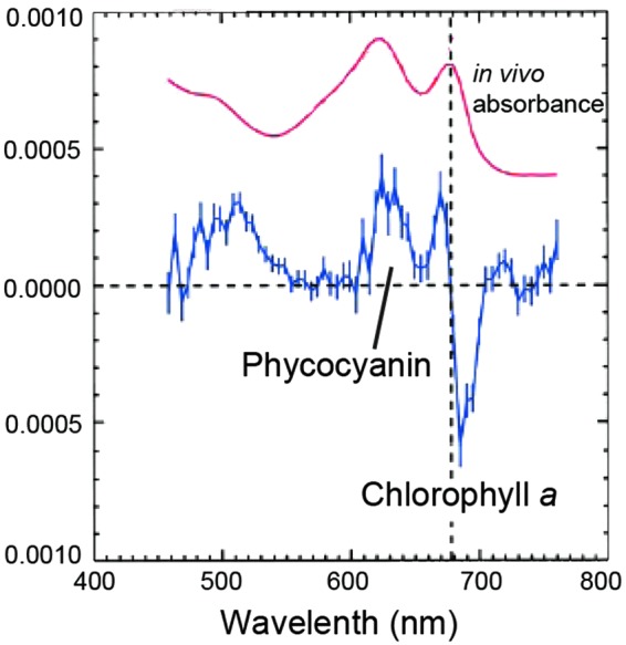
Reflected circular polarization spectrum of a planktonic suspension of a marine cyanobacterium (center plot). The in vivo absorption spectrum is shown in the upper plot and is arbitrarily scaled. The absorbance maxima of Chl a (435, 680 nm), phycocyanin (620 nm), and carotenoids (∼450 nm) are visible. The large feature in the circular polarization spectrum corresponds to the absorbance by chiral aggregates of Chl a and proteins. After Sparks et al. (2009b).
Chirality can in principle be remotely detected on planetary scales by linear and circular polarization spectroscopy. Linear polarization (light waves that oscillate in single direction rather than rotating in a plane as the light travels) has been used in biochemical studies to characterize, for example, the orientation of pigment molecules in cells, while circular polarization has been used to examine excitonic coupling in pigment–protein complexes (Garab and van Amerongen, 2009). Investigators have examined whether pigment signatures in linear polarization spectra could serve as remotely detectable signs of life (Berdyugina et al., 2016). The degree of linear polarization is correlated with the strength of pigment absorption, producing an inverted effect relative to the VRE in which the degree of linear polarization is high at visible wavelengths and low in the NIR (Peltoniemi et al., 2015; Berdyugina et al., 2016). However, it has been shown that abiotic environmental factors such as mineral dust (West et al., 1997), scattering by particles in the atmosphere (Shkuratov et al., 2006), and the molecular absorption by gases (Stam, 2008; Takahashi et al., 2013; Miles-Páez et al., 2014) can also produce positive linear polarization signals. As a result, the biotic and abiotic inputs of linear polarization spectra must be disentangled. In contrast, the degree of circular polarization is more directly tied to the optical activity of amino acids and pigments, making it a more specific biosignature (Sparks et al., 2009a, 2009b; Patty et al., 2017). However, of concern is the relatively weak signal strength of the circular polarization signal of photosynthetic pigments, which is on the scale of 10−2–10−4 (Sparks et al., 2009a, 2009b). In addition, the degree of polarization responds to the physiological state of the organisms, potentially adding a predictable temporal variation to the polarization signature (Patty et al., 2017).
Sterzik et al. (2012) measured the linear polarization of Earthshine and found that for one observation window, the data were best fit with a model containing 10–15% noncloud covered vegetation. A circular polarization signal was not detected. However, it is not known whether light reflecting from the dusty surface of the Moon interfered with the polarization signal. Linear and circular polarization signatures providing an additional, potentially determinative, dimension for biosignature analysis are interesting topics for future study.
5.6. Fluorescence and bioluminescence
Photons directly sourced from organisms could represent another category of surface biosignature. One manifestation of this phenomenon is chlorophyll autofluorescence, which has been observed by low Earth-orbiting satellites with the aim of characterizing plant health and primary productivity (Joiner et al., 2011). Autofluorescence is the reprocessing of absorbed higher energy photons into emitted lower energy photons. Autofluorescence is observed in abiotic materials such as fluorite and calcite, so biogenicity must be determined from the nature of the fluorescence spectrum. Chlorophyll fluorescence is a signature of photosynthesis believed to reduce physiochemical stress on the organism (Papageorgiou and Govindjee, 2007). The fluorescence spectrum of Chlorophyll a consists of broad emission from 640 to 800 nm with maxima located at 685 and 740 nm (Meroni et al., 2009). Because fluorescence is the instantaneous reprocessing of absorbed light, it occurs only on the day side of the planet, and thus, the fluorescence signature must be measured against reflected light from the Sun [or star(s)]. The chlorophyll fluorescence signature over vegetated areas constitutes about 1–5% of the total spectral flux at the fluorescing wavelengths (Meroni et al., 2009; Joiner et al., 2011). To detect the fluorescence component amid contamination from reflected light, observations focus on telluric (e.g., the O2-A band) or reflected solar absorption bands (e.g., H-alpha), which are partially filled in by the fluorescent emission flux. The fluorescence flux constitutes a proportionally larger fraction of the total flux at these wavelengths (Meroni et al., 2009; Joiner et al., 2011). Fluorescence as an adaptation in response to high-UV flare events has been proposed as a potentially temporal biosignature for planets orbiting M dwarf stars (O'Malley-James and Kaltenegger, 2016). To detect biological fluorescence will be very challenging and would require signal-to-noise ratios higher than for most features thus far discussed.
Bioluminescence, in contrast to fluorescence, involves the direct production of photons through the oxidation of a luciferin (“light-bringing”) molecule (Haddock et al., 2010). Luciferin is a general category of light-emitting molecules involved in bioluminescence, produced by a wide variety of lineages that independently evolved bioluminescence, including species of bacteria, fish, eukaryotic planktons, and insects (Haddock et al., 2010). Most luciferin molecules have a peak emission wavelength in the green region of the visible spectrum (in contrast to chlorophyll fluorescence that peaks in the red). Vibrio bacteria in the ocean can generate a faint bioluminescent glow covering up to 10,000–20,000 km2. Called a “Milky Sea” effect, this glow can be characterized by Earth observing satellites (Miller et al., 2005). The potential of bioluminescence to serve as an exoplanet biosignature is poorly studied and constrained. However, it is important to point out that bioluminescence will be limited by the productivity and ecology of the biosphere and more stringently on its evolutionary function, which may vary but will likely be very challenging to detect on exoplanets due to signal-to-noise constraints.
6. Temporal Biosignatures
Temporal biosignatures are measurable time-dependent modulations that indicate the presence of a biosphere acting on a planetary environment (e.g., Meadows, 2006, 2008). These temporal modulations can take the form of oscillations in gas concentrations or the surface spectral albedo of the planet. They may even cause the direct emission of light by organisms (e.g., bioluminescence, see Section 5.6) provided there is a direct link between the detectable change (e.g., stellar activity) and biological action. The most commonly referenced temporal signature is the seasonal change in CO2 concentration in Earth's northern hemisphere as a response to the changing productivity of the land biosphere as a function of temperature and insolation (e.g., Keeling et al., 1976). Seasonal changes may be driven primarily by obliquity, as on Earth, or by orbital eccentricity where the effects from changing planet–star distance would dominate. However, a temporal biosignature need not be seasonal in cadence but could be diurnal or act in response to another measurable environmental variable. Temporal biosignatures have been less studied than other types of biosignatures, in part, because of the complexity required to model them with additional variables such as the axial tilt, orbital eccentricity, and surface heterogeneity of the planet likely playing key roles. In addition, it is important to note that temporal changes must be present in the disk average to be observable and therefore will be dependent on observer/target viewing geometries in additional to the static properties and intrinsic changes of the planetary environment, particularly for those seasonal changes driven by obliquity. For example, an equator-on view will average changes in both visible hemispheres and require hemispherical asymmetries for a seasonal change driven by obliquity to be observed. However, in the other extreme, a near pole-on view will primarily include only one hemisphere, and so a hemispherical dichotomy would not be necessary to observe seasonal changes. Most scenarios will reside between these extremes. Of course, temporal changes driven by eccentricity would also not require specific hemispherical dichotomies, although they may complicate interpretations should they exist. In this section, we present an overview of temporal biosignatures based primarily on deriving inferences from Earth system studies and observations.
6.1. Oscillations of atmospheric gases
Earth's biosphere imparts modulations on several key spectrally active gases in the atmosphere, including CO2, O2, O3, and CH4 (Fig. 15). The most well known of these is the seasonal oscillation in CO2 due to growth and decay of vegetation on land (Keeling, 1960; Hall et al., 1975; Keeling et al., 1976). The CO2 content of the atmospheres decreases in the spring season as CO2 is fixed into organic matter by vegetative growth, then begins to rise in fall and winter as CO2 consumption slows and plant matter decays. The magnitude of the change is dependent on hemisphere and latitude. In the northern hemisphere, the amplitude of the CO2 oscillation ranges from ∼3 ppm near the equator to ∼10–20 ppm at high latitudes (Keeling et al., 1996). Overall, the amplitude is far greater in the northern hemisphere than the southern due to its substantially greater continental area (and thus vegetative cover). The seasonal variation in O2 concentrations is linked to CO2 consumption by the photosynthesis net reaction (CO2 + H2O → CH2O + O2) and the reverse decomposition net reaction (CH2O + O2 → CO2 + H2O), so that oscillations in O2 are anticorrelated with those of CO2. The absolute amplitude of O2 variability (in ppm or per moles), however, is larger than that of CO2 because CO2 is substantially more soluble in seawater (Keeling and Shertz, 1992). The lower solubility of O2 also explains why its magnitude of seasonal variability is comparable between hemispheres, with an amplitude of about ∼50 ppm at midlatitudes (Keeling et al., 1998).
FIG. 15.
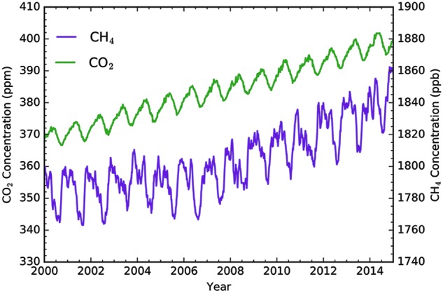
Gas abundance oscillations as a possible temporal biosignature. Volume mixing ratio measurements of CH4 and CO2 from the National Oceanic and Atmospheric Association (NOAA) at Mauna Loa, HI from 2000 to 2015 (Dlugokencky et al., 2017; Thoning et al., 2015). The seasonal variations in both gases are partially reflective of the seasonal change in the productivity of the biosphere in the northern hemisphere (the secular increase in both gases is attributable to industrial emissions). These data were obtained from the NOAA's Earth System Research Laboratory (www.esrl.noaa.gov).
Seasonal variability in CH4 is more complicated. The highest CH4 levels occur in the late fall and early spring, but CH4 concentrations fall in the summer and winter, reaching an annual minimum in northern summer and a more muted minimum in winter (Rasmussen and Khalil, 1981). The variation in CH4 concentrations is only partly biogenic (i.e., controlled by biological sources and sinks); instead, its temporal oscillations are dominantly controlled by interactions with OH ions that destroy it (OH + CH4 → CH3 + H2O). This destructive OH is ultimately sourced from tropospheric H2O [mostly via H2O + O(1D) →2OH], which increases in summer (due to increased water evaporation) and decreases in winter, so that the CH4 abundance in the atmosphere is more strongly correlated with surface temperature (hence H2O) and solar zenith angle [hence O(1)D] than instantaneous release from the biosphere (Khalil and Rasmussen, 1983). This example illuminates an interesting scenario through which a gas is primarily sourced from biological activity, but its seasonal modulation is abiotic. O3 on Earth also displays a dominantly abiotically driven seasonal variability with a midlatitude early spring maximum due to suppressed photolytic destruction in winter, which has an amplitude of about 30% in the total column value (WMO, 1994). Temporal variation in the O3 column can arise due to both photochemical and dynamical effects.
Detecting gas oscillations of the same magnitude as those of Earth's modern biosphere will be quite challenging and likely beyond the capability of next-generation observatories. CO2 and CH4 vary on the order of 1–3% (and CH4's variation is only partly biogenic), while O2 varies by 50 ppm against a 21% background, or by ∼0.02%. In addition, target absorption bands (such as CO2's 15 μm band) will not vary linearly with abundance if they are saturated; thus, the measurable spectral variability may be less than this. In ideal circumstances, temporal gas oscillations will occur at background gas abundances that are detectable, but not saturated, and impart measurable spectral variability. In addition, potential false positives, such as seasonal sublimation of CO2 ice, must be ruled out but could be in cases where planetary temperature ranges are known (i.e., as seen on Mars). Further work is required to illuminate the cases in which a biosphere could produce measurable and inferable modulations of gases linked to metabolism.
6.2. Oscillations in surface signatures
Changes in surface albedo or the spectrum of reflected light from the surface represents another form of temporal biosignature. For example, the VRE signature is temporally variable because of the seasonal growth and senescence of green vascular plants on continents (Fig. 16). The temporal variability of the “edge” signature, in conjunction with seasonal changes at the same phase, could enhance the case for the biological origin of the signature. Furthermore, the NDVI of stressed and dead vegetation has a lower value than living vegetation, because chlorophyll absorption is weaker (making the plant more reflective in the visible), while desiccated vegetation reduces the NIR reflectivity (Tucker, 1979). The circular polarization fingerprint of vegetation also changes as a function of physiological stress (Patty et al., 2017) and may be an additional temporal signature in phase with reflectivity changes. Changing external conditions may also induce changes in pigmentation to acclimate the organisms to temperature or irradiation stressors (e.g., Archetti et al., 2009). It is important to note that microbial mats also experience seasonal alterations in pigmentation (Nicholson et al., 1987). Time-dependent changes in bioluminescent or biological fluorescence could also serve as a temporally variable surface biosignature (Section 6.3). Necessarily, seasonal changes in the reflection signature will be smaller than or equal to the maximal steady-state spectral signature, so greater signal-to-noise will be required to measure them. As stated previously, temporal biosignatures need not necessarily be driven by seasonal changes, but could also occur in phase with rotation or other dynamical processes. For example, tidally induced algal blooms have been posited as a potential remote temporal biosignature (Lingam and Loeb, 2017).
FIG. 16.

Seasonal change in global NDVI. These vegetation maps were generated from data taken by the Moderate Resolution Imaging Spectroradiometer (MODIS) on board NASA's Terra satellite and converted to NDVI values. Significant seasonal variations in the NDVI are apparent between northern hemisphere summer (July 2014; top) and winter (February 2015; bottom). Image credit: Reto Stockli, NASA Earth Observatory Group, using data from the MODIS Land Science Team (http://neo.sci.gsfc.nasa.gov).
7. Assessing Biosignature Plausibility
Methods for assessing biosignature plausibility are important for two primary reasons. First, there is the problem of interpretation. Because of potential false positives, the detection of a single gas, and perhaps even some combination of gases, is unlikely to constitute robust evidence of life alone. Therefore, whether we attribute measured spectral properties of an exoplanet to the presence of life requires a scheme for evaluating the planetary context to determine the likelihood that a biological process is involved. Second, we wish to prospectively determine the best biosignatures to search for as we design the technological capabilities to characterize exoplanets for evidence life. This goal is essential, as different gases and surface features have spectral features at different and often widely separated spectral locations that will be impossible for any single instrumental configuration to span. Below, we briefly review three potential methods for evaluating biosignature plausibility: chemical disequilibrium, biomass estimation, and applications of network theory to biosignatures.
7.1. Chemical disequilibrium
It has long been recognized that the chemical composition of Earth's atmosphere is far from equilibrium. Much effort has been directed at studying this disequilibrium to understand the biological inputs that can allow for, for example, the simultaneous existence of CH4 and O2. These two gases should rapidly oxidize to CO2 and H2O, so their persistent presence suggests a continual resupply of both gases from biological sources. This state of disequilibrium (sometimes termed “redox disequilibrium”) has been proposed as a biosignature (Lederberg, 1965; Lovelock, 1965; Hitchcock and Lovelock, 1967; Sagan et al., 1993), and is a chemical signature that can be used to guide the search for life in exoplanet atmospheres. Much effort has been directed at quantifying the degree of disequilibrium to try to disentangle abiotic (e.g., photochemistry) and biotic (methanogenesis and OP) inputs. However, Simoncini et al. (2013) found that rather than quantifying the distance from disequilibrium, a useful parameter to examine is the power required to drive disequilibrium. If the residence time of the gases in the atmosphere is long, a relatively small amount of energy is required to establish a high degree of disequilibrium. Conversely, if the residence time of the gases is short, and the disequilibrium high, then a high degree of power, likely biological, is required to maintain that atmospheric composition.
The O2-CH4 (and the related O3-CH4) disequilibrium pair is the most highly cited and explored biosignature couple in Earth's atmosphere (e.g., Sagan et al., 1993) because it requires large fluxes of CH4 (as the less abundant gas) to maintain, fluxes that are believed to be incompatible with abiotic sources. However, it is important to note that CH4 is both substantially less abundant and less spectrally detectable in Earth's modern atmosphere than O2. In addition, these two gases absorb most strongly at disparate wavelengths—O2's strongest feature is in the optical at 0.76 μm, while CH4's strongest absorption features lie deep into the NIR and MIR wavelength regimen. These challenges and others pose potential obstacles for observing the O2-CH4 biosignature couple in exoplanets (see Section 8 below).
While references to chemical disequilibrium in Earth's atmosphere typically focus on the CH4/O2 disequilibrium pair, Krissansen-Totton et al. (2016a) recently found that the largest disequilibrium in the Earth system in terms of free energy is the coexistence of substantial quantities of free O2 and N2 in the atmosphere in contact with a liquid water ocean. In an equilibrium state, N2 and O2 would be converted by, for example, lightning into NOx, in turn oxidized into HNO3, which is rapidly washed out of the atmosphere to form the thermodynamically stable NO3− in the ocean. The fact that substantial quantities of both N2 and O2 exist simultaneously within the atmosphere–hydrosphere system suggests that nonequilibrium (living) processes are acting to reprocess these gases. To verify the presence of this potential disequilibrium signature, O2, N2, and a liquid water ocean would need to be detected. This combination is hypothetically detectable with known methods, through the optical-NIR absorption features of O2 (given in Section 4.2.1), ocean glint inferred from departures of Lambertian reflectance as the planet spectrum evolves with phase (e.g., Robinson et al., 2010, 2014), and detection of N2 through N2-N2 collisional absorption near 4.1 μm (Schwieterman et al., 2015b) or retrievals of atmospheric mass through Rayleigh scattering or estimates of atmospheric refraction that can constrain N2 abundances.
7.2. Biomass estimation
Because of the abundance of water as an electron donor for photosynthesis and the availability of light on Earth, OP dominates primary productivity and it is currently responsible for gross fixation of 100–175 Pg of inorganic carbon per year (Field, 1998; Welp et al., 2011). Currently, ocean and land primary productivity account each for approximately half the global total. Oxygenic phototrophs, such as cyanobacteria on the early Earth, possibly generated comparable biomass in shallow nearshore areas, continental settings, and possibly in the open ocean (e.g., Garcia-Pichel et al., 2003). Such extensive areal coverage may bode well for detection of pigmented surface biosignatures on an inhabited exoplanet. In contrast, anoxygenic phototrophs are usually limited by the environmental availability of electron donors (e.g., H2, H2S, Fe2+). Initial calculations suggest that these types of communities might be two to three orders of magnitude less productive (with less surface biomass generated) than modern oxygenic ones (Des Marais, 2000; Kharecha et al., 2005), possibly making their detection on exoplanets more difficult.
Beyond surface biosignatures whose detectability depends on percent areal coverage on the continents, near shore areas, and ocean, Seager et al. (2013a) developed a model to assess the detection of biogenic gases in the atmosphere that is linked to biomass estimates based on thermodynamic calculations. This model is not meant to apply to all types of biosignatures but primarily to biogenic gases that are by-products of metabolisms that obtain energy from chemical potential gradients in the environment and to biochemicals that have specialized functions other than energy capture. In these cases, the amount of biomass correlates with amount of activity. A high cycling rate otherwise does not necessarily correlate with a high net flux or a high biomass stock. Therefore, the model does not apply to oxidizing gases resulting from biomass building processes in which a large stock of inactive biomass or fixed carbon may be stored. A primary example is the biogenic gas O2 from OP, for which large organisms such as trees may have a large carbon stock in woody tissue, while active foliage biomass is relatively small. At the planetary scale, O2 has an extremely low net flux, and its large atmospheric accumulation on Earth is the result of long-term storage of fixed carbon in ocean sediments and soils on land (Catling, 2014).
For the relevant biological processes mentioned above, this kind of biomass estimation model can establish first-order estimates for the plausible biogenicity of these gases, rather than adopting terrestrial fluxes. Importantly, this type of framework can be employed as a plausibility assessment of the utility of a potential biosignature gas for a specific planet–star combination, given the prediction of the biomass necessary to produce a detectable signature. In this scenario, the UV properties of the host star (which drives photochemistry) and the observing capabilities of the telescope are input parameters. The flux of a given biosignature gas (e.g., N2O, CH3Cl) is increased until a detectability threshold is met. That flux is linked to a thermodynamic estimate of biomass, which can then be evaluated for plausibility. This was done for a range of scenarios presented in Seager et al. (2013a).
7.3. Applications of network theory to biosignatures
Another possibility for detecting life on an exoplanet is to look at the interactions between atmospheric constituents. By using techniques developed for graph theory and network analysis, the set of reactions present in an atmosphere can be converted into a chemical reaction network (CRN). In a CRN, chemical species are represented by nodes in a graph, with the reactions between them forming “edges,” or connections between these nodes. The topological properties of the resulting network can then be measured and may include assortativity, which is the measurement of a node to attach to others that are similar in some way; average clustering coefficient, which indicates the degree that nodes in a graph tend to cluster together; and mean degree, or the average number of a degrees a node in the network has. In addition, other statistical properties, such as the degree distribution (how edges are distributed across the population of nodes, and how this distribution scales), can also provide insights into the structure of the network.
Preliminary studies by Solé and Munteanu (2004) examined the CRNs of every significant planetary atmosphere in the Solar system, and found that Earth's was unique: its topology displays a hierarchical and modular structure, whereas the CRNs of other planets appear more random. Further investigation by Holme et al. (2011) found similar results, suggesting that the degree, distribution, and scaling of Earth's reaction network are more like those of metabolic reaction networks than other planetary atmospheres. In addition, Solé and Munteanu (2004) reported that Earth's atmosphere is more modular, also more like biology.
Holme et al. (2011) further speculated that the differences between the network structure of Earth's atmosphere and others may be due to the comparatively small size of the data set for most planetary CRNs. Nonetheless, given that similar topological signatures have already been identified in biological networks (Jeong et al., 2000)—a feature that in and of itself has been suggested as a potential biosignature (Jolley and Douglas, 2012)—and that the topology also appears to influence chemical disequilibrium in the atmosphere (Estrada, 2012), these findings suggest the possibility that the presence of a global biosphere influences the topology of a planet's atmospheric CRN in a significant, potentially detectable way.
While further study is required to validate this technique (especially in terms of comparing the topology of nonbiological systems, such as hot Jupiters) and establish its sensitivity, it holds tremendous promise as a tool for assessing exoplanet habitability and potential influence of a global biosphere. A following companion article contains further discussion of this topic (Walker et al., 2018).
8. Cryptic Biospheres: “False Negatives” for Life?
While it can be argued that the evidence for life on modern Earth is strongly remotely detectable from the presence of abundant O2, this will not necessarily be the case for every inhabited planet. Biospheres that persist only on chemosynthetic metabolisms will have orders of magnitude lower productivity than photosynthetic ones (Des Marais, 2000), and chemosynthesis reduces chemical disequilibrium rather than enhancing it (Seager et al., 2012). Moreover, many known microorganisms and even entire ecosystems are cryptic to surface spectral detection, such as endolithic communities. Photosynthetic endoliths may live in fractures under rock surfaces, ruling out surface biosignatures, although they may emit O2 if oxygenic (Cockell et al., 2009a). Subsurface oceans in the icy moons of the outer Solar system may host redox-driven microbial biospheres cryptic to remote detection (e.g., Lipps and Reiboldt, 2005) with confirmation only possible with in situ exploration.
Studies of the early Earth, a persistently habitable and inhabited planet, likewise sound a cautionary note for expectations of the general detectability of exoplanet biosignatures, particularly for the utility of the O2-CH4 biosignature couple (Reinhard et al., 2017; see Fig. 17). The Archean Earth's atmosphere was significantly more reducing than today's and contained no detectable O2 or O3. While the Archean eon's (4.0–2.5 Ga) atmosphere likely contained significant detectable amounts of CH4, it is unclear whether this alone would be an unequivocal sign of life (Arney et al., 2016). The Proterozoic eon (0.5–2.4 Ga) has been viewed in recent studies as perhaps an archetypical model for a highly detectable disequilibrium biosphere, believed to have both detectable O2 (10%) and much higher CH4 (∼100 ppm) than modern Earth (e.g., Kaltenegger et al., 2007). However, recent geochemical evidence based on chromium isotopes suggests that Proterozoic O2 was quite low (perhaps <0.1% of PAL) (Planavsky et al., 2014b; Lyons et al., 2014), while biogeochemical modeling studies of sulfate cycling in the ancient ocean suggest that CH4 was also much lower (1–10 ppm) (Olson et al., 2016). If these estimates of low O2 are correct, Fig. 17 shows that O3 would have resided at the cusp of detectability during the mid-Proterozoic eon, and would have only been potentially detectable in the UV (Reinhard et al., 2017). (Although the O3 concentration is relatively insensitive to O2 abundances over several orders of magnitude, this relationship breaks down at the lowest published limits for Proterozoic O2; i.e., pO2 < 0.1% PAL).
FIG. 17.

Potential “false negatives” for remote life detection. Left: conceptual figure illustrating the difficulty of detecting the O2-CH4 disequilibrium signature through Earth history. Right: synthetic spectra, at 1 cm−1 resolution, of the O3 Huggins–Hartley band (0.25 μm), O2-A band (0.76 μm), and 1.65 μm CH4 band at different geologic times assuming gas abundances consistent with geochemical proxies and/or biogeochemical modeling constraints. Black represents no absorption by the indicated gas, red a lower limit, and blue an upper limit, given reasonable uncertainties in geochemical proxies. Adapted with permission from Reinhard et al. (2017).
As vascular land plants have only existed for the last ∼470 million years (Kenrick and Crane, 1997), surface signatures of life on early Earth may have been significantly muted unless microbial mats or other microbial structures had significant areal extent comparable to, or larger than, vegetation today (e.g., Sanromá et al., 2013). There is evidence of microbial mats inhabiting land surfaces over 1 billion years ago (Horodyski and Knauth, 1994; Prave, 2002; Beraldi-Campesi, 2013). Investigators have been exploring surface biosignatures resulting from anoxygenic phototrophs and cyanobacteria growing in continental, marine marginal, and open ocean settings and are addressing the percent areal coverage necessary for detection through different atmospheric compositions and cloud coverage levels (Sanromá et al., 2014; Parenteau et al., 2015). However, the possibility exists that significant portions of Earth history, if not the entire window before the second rise of O2 (∼0.54 Ga), could represent a potential “false negative” for remotely detectable life, at least through O2 and the O2-CH4 disequilibrium couple (Reinhard et al., 2017) and perhaps for surface signatures as well. No matter how common or rare life is in the Universe, it is unlikely that every inhabited planet will have remotely detectable biosignatures (Cockell, 2014). This lesson from Earth history should be kept in mind when creating statistical frameworks for the prevalence of life given negative results and when estimating biosignature yields for surveys of candidate exoEarths (Stark et al., 2014, 2016; Léger et al., 2015). In addition, these results further reinforce the importance of broad spectral capabilities (UV-VIS-NIR-MIR) and high spectral resolving power of exoplanet characterizing missions and facilities, which would enhance the chance of characterizing biosignatures on worlds such as the early Earth.
9. Prospects for Detecting Exoplanet Biosignatures
The actual detectability of any of the biosignatures presented in this review will be related to a variety of factors, including those related to the observing telescope architecture (e.g., aperture, coronagraph throughput, instrument sensitivity), target system distance and qualities (e.g., spectral type, exozodiacal light), planetary parameters (e.g., size, albedo, composition), and the accessible spectral range that will depend both on variables related to the telescope and target system. In general, the detection of exoplanet biosignatures is expected to follow a trajectory where interesting and accessible (via remote sensing) planet candidates are identified, for example, by the TESS mission (2018 launch; Ricker et al., 2014; Sullivan et al., 2015), the PLATO 2.0 mission (2026 launch; Rauer et al., 2014), or ground-based radial velocity (RV) or transit surveys, followed by intensive characterization by the JWST mission (2020 launch, Deming et al., 2009; Stevenson et al., 2016), extremely large ground-based telescopes (ELTs; first light in mid-2020s), or a future direct-imaging mission such as the envisioned LUVOIR/HDST or HabEx class missions (∼2030s) (Dalcanton et al., 2015; Mennesson et al., 2016).
In addition, ELTs and LUVOIR/HabEx would have the capability to both independently identify initial candidates and characterize them in search of biosignatures. JWST is likely to characterize only a handful of potentially habitable planets with the fidelity required to detect biosignature gases or signs of habitability (Cowan et al., 2015). Importantly, transmission spectroscopy can only probe for atmospheric habitability markers and biosignatures at a single phase, excluding the detectability of all potential surface biosignatures and most proposed temporal biosignatures. With a planned 2025 launch, WFIRST could potentially characterize Earth-sized planets in the HZs of Alpha Centauri A and B, and possibly a handful of other nearby stars, if flown with a star shade and depending on the in-flight performance of instrumentation (Spergel et al., 2015). The available wavelength range is an essential consideration for exoplanet biosignature assessment, because many gases will not create measurable spectral impacts in the UV-visible range. There is no space-based mission currently being studied that will possess the capability of characterizing the MIR spectrum of an Earth-sized planet, although the TPF-I concept was studied in the past (Beichman et al., 2006; Lawson et al., 2006). However, a combination of LUVOIR/HDST, which may cover a spectral range inclusive of 0.2–2.0 μm, and ground-based telescopes sensitive in the MIR, could cover most of the electromagnetic spectrum relevant for biosignatures.
A companion article (Fujii et al., 2018) discusses upcoming missions and observatory capabilities in far more extensive detail, and provides a robust time line for expected biosignature detection capabilities. In addition, other companion articles (Catling et al., 2018; Walker et al., 2018) provide a foundation for robust frameworks for defining and evaluating biosignature detections.
10. Summary
We have provided an overview of potential signs of life on exoplanets, including gaseous, surface, and temporal biosignatures. The most detectable signs of life will likely result from a photosynthetic biosphere. Biosignature gases in Earth-like (N2-H2O-CO2) atmospheres include O2, O3, CH4, C2H6, N2O, CH3Cl, CH3SH, DMS, and DMDS, although any individual gas alone is likely insufficient for biosignature confirmation due to potential false positive scenarios. Organic aerosols may be suggestive of life in atmospheres high in CO2, while NH3 may be a biosignature gas in H2-dominated terrestrial atmospheres, providing false positives can be ruled out. Overlaps between absorbing wavelengths of key gases (e.g., O3 with CO2 and CH3Cl) and the potential abiotic production of certain gases caution against reliance on any single spectral feature, and indicate a wide spectral range is necessary for biosignature characterization. The interpretation of gaseous signatures will depend on the redox state of the atmosphere, which will determine which disequilibrium signatures are feasible.
The environmental context will also play a key role in interpreting potential gaseous biosignatures. For example, the N2-O2-ocean disequilibrium signature requires the detection of surface liquid water, perhaps through glint. The most well-studied surface biosignature continues to be the VRE. Detecting an exact analogue to Earth's disk-averaged VRE signature will likely require 1% spectrophotometric precision and ∼10% or more cloud-free surface coverage of exo-vegetation. Analogues to the VRE, “edge” biosignatures, may be produced by photosynthetic or nonphotosynthetic pigments or structures and occur throughout the visible and NIR spectrum. Linear and circular polarization signatures and contextual information could be used to rule out false positives for surface biosignatures. Temporal biosignatures may include seasonal modulation in biologically mediated gases such as CO2 or O2, changes in surface signatures such as analogues to the VRE, or direct emission of light by organisms (e.g., bioluminescence, fluorescence). In general, temporal biosignatures are less well studied than gaseous or surface biosignatures and additional work is necessary to elucidate the range of applicability for this category of signatures.
Earth history suggests that not all inhabited planets with global biospheres will necessarily have remotely detectable signs of life, and that broad spectral capabilities and high resolving power will increase the chances of success. Updates to the disequilibrium framework, new biomass estimation models, discoveries of greater diversity of photosystems in OP, and network theory applied to atmospheric biosignatures offer novel or evolving frameworks, which may enhance our ability to characterize and correctly interpret exoplanet biosignatures in the future.
Abbreviations Used
- 1D
one-dimensional
- 3D
three-dimensional
- C2H6
ethane
- CH3
methyl
- CH3SH
methanethiol
- CH4
methane
- CRN
chemical reaction network
- DMDS
dimethyl disulfide
- DMS
dimethyl sulfide
- ELTs
extremely large ground-based telescopes
- GCM
General Circulation Model
- GOE
Great Oxidation Event
- H2S
hydrogen sulfide
- HNO3
nitric acid
- HZ
habitable zone
- JWST
James Webb Space Telescope
- MIR
midinfrared
- N2O
nitrous oxide
- NDVI
Normalized Difference Vegetation Index
- NExSS
Nexus for Exoplanet System Science
- NO3−
nitrate
- NOX
nitrogen oxides
- NUV
near-ultraviolet
- OH
hydroxyl
- OP
oxygenic photosynthesis
- PAL
present atmospheric level
- PSI
photosystem I
- PSII
photosystem II
- RC
radiative–convective
- SETI
Search for Extraterrestrial Intelligence
- SO2
sulfur dioxide
- TPF-I
Terrestrial Planet Finder—Infrared mission
- UV
ultraviolet
- UV-VIS-NIR-MIR
ultraviolet, visible, near-infrared, and midinfrared
- VPL
Virtual Planetary Laboratory
- VRE
vegetation red edge
Acknowledgments
The authors thank the NASA Astrobiology Program and the Nexus for Exoplanet System Science (NExSS) for their support of the NExSS Exoplanet Biosignatures Workshop. Conversations at this workshop, held in the summer of 2016 in Seattle, formed the basis for the drafting of the five review articles in this issue. They also thank Mary Voytek, the senior scientist of NASA Astrobiology, for her leadership of NExSS and her feedback on our organization of the workshop and article. E.W.S. is additionally grateful for support from the NASA Postdoctoral Program, administered by the Universities Space Research Association. This work was also supported by the NASA Astrobiology Institute, including the VPL under Cooperative Agreement Number NNA13AA93A and the Alternative Earths team under Cooperative Agreement Number NNA15BB03A. S.D. acknowledges support from NASA exobiology grant NNX15AM07G. The research of R.H. was carried out at the Jet Propulsion Laboratory, California Institute of Technology, under a contract with the National Aeronautics and Space Administration. The authors thank the following individuals for helpful comments, suggestions, and discussion during the community review period: Tanai Cardona, Anthony Del Genio, Stephen Kane, and Enric Pallé. Finally, the authors are thankful for the helpful comments from two anonymous referees, which allowed us to further improve the paper.
Author Disclosure Statement
No competing financial interests exist.
The band gap energy is the difference in energy between mixed orbitals where strong covalent bonds are formed. The lower energy filled orbital can have an electron excited into the higher energy orbital, and the energy gap corresponds to the photon energy required.
References
- Abe Y., Abe-Ouchi A., Sleep N.H., and Zahnle K.J. (2011) Habitable zone limits for dry planets. Astrobiology 11:443–460 [DOI] [PubMed] [Google Scholar]
- Airapetian V.S., Glocer A., Gronoff G., Hébrard E., and Danchi W. (2016) Prebiotic chemistry and atmospheric warming of early Earth by an active young Sun. Nat Geosci 9:452–455 [Google Scholar]
- Airapetian V.S., Glocer A., Khazanov G. V., Loyd R.O.P., France K., Sojka J., Danchi W.C., and Liemohn M.W. (2017) How hospitable are space weather affected habitable zones? The role of ion escape. Astrophys J 836:L3 [Google Scholar]
- Akeson R.L., Chen X., Ciardi D., Crane M., Good J., Harbut M., Jackson E., Kane S.R., Laity A.C., Leifer S., Lynn M., McElroy D.L., Papin M., Plavchan P., Ramírez S. V, Rey R., von Braun K., Wittman M., Abajian M., Ali B., Beichman C., Beekley A., Berriman G.B., Berukoff S., Bryden G., Chan B., Groom S., Lau C., Payne A.N., Regelson M., Saucedo M., Schmitz M., Stauffer J., Wyatt P., and Zhang A. (2013) The NASA exoplanet archive: data and tools for exoplanet research. Publ Astron Soc Pac 125:989–999 [Google Scholar]
- Allakhverdiev S.I., Kreslavski V.D., Zharmukhamedov S.K., Voloshin R.A., Korol'kova D.V., Tomo T., and Shen J.R. (2016) Chlorophylls d and f and their role in primary photosynthetic processes of cyanobacteria. Biochemistry (Mosc) 81:201–212 [DOI] [PubMed] [Google Scholar]
- Allen M., Yung Y.L., and Waters J.W. (1981) Vertical transport and photochemistry in the terrestrial mesosphere and lower thermosphere (50–120 km). J Geophys Res 86:3617 [Google Scholar]
- Aneja V.P. and Cooper W.J. (1989) Biogenic sulfur emissions. In Biogenic Sulfur in the Environment, edited by Saltzman E.S. and Cooper W.J., Washington, DC, Vol. 393, pp 2–13. doi: 10.1021/bk-1989-0393.ch001 [DOI] [Google Scholar]
- Anglada-Escudé G., Amado P.J., Barnes J., Berdiñas Z.M., Butler R.P., Coleman G.A.L., de la Cueva I., Dreizler S., Endl M., Giesers B., Jeffers S. V., Jenkins J.S., Jones H.R.A., Kiraga M., Kürster M., López-González M.J., Marvin C.J., Morales N., Morin J., Nelson R.P., Ortiz J.L., Ofir A., Paardekooper S.-J., Reiners A., Rodríguez E., Rodrίguez-López C., Sarmiento L.F., Strachan J.P., Tsapras Y., Tuomi M., and Zechmeister M. (2016) A terrestrial planet candidate in a temperate orbit around Proxima Centauri. Nature 536:437–440 [DOI] [PubMed] [Google Scholar]
- Archetti M., Döring T.F., Hagen S.B., Hughes N.M., Leather S.R., Lee D.W., Lev-Yadun S., Manetas Y., Ougham H.J., Schaberg P.G., and Thomas H. (2009) Unravelling the evolution of autumn colours: an interdisciplinary approach. Trends Ecol Evol 24:166–173 [DOI] [PubMed] [Google Scholar]
- Ardanuy P.E., Han D., and Salomonson V. V. (1991) The moderate resolution imaging spectrometer (MODIS) science and data system requirements. IEEE Trans Geosci Remote Sens 29:75–88 [Google Scholar]
- Arney G., Meadows V., Crisp D., Schmidt S.J., Bailey J., and Robinson T. (2014) Spatially-resolved measurements of H2O, HCl, CO, OCS, SO2, cloud opacity, and acid concentration in the Venus near-infrared spectral windows. J Geophys Res Planets 119: 1860–1891. doi: 10.1002/2014JE004662 [DOI] [Google Scholar]
- Arney G., Domagal-Goldman S.D., Meadows V.S., Wolf E.T., Schwieterman E., Charnay B., Claire M., Hé E., Trainer M.G., Hébrard E., and Trainer M.G. (2016) The pale orange dot: the spectrum and habitability of hazy Archean Earth. Astrobiology 16:873–899 [DOI] [PMC free article] [PubMed] [Google Scholar]
- Arney G.N., Meadows V.S., Domagal-Goldman S.D., Deming D., Robinson T.D., Tovar G., Wolf E.T., and Schwieterman E. (2017) Pale orange dots: the impact of organic haze on the habitability and detectability of earthlike exoplanets. Astrophys J 836:49 [Google Scholar]
- Arney G., Domagal-Goldman S.D., and Meadows V.S. (2018) Organic haze as a biosignature in anoxic Earth-like atmospheres. Astrobiology 18:311–329 [DOI] [PMC free article] [PubMed] [Google Scholar]
- Arnold L. (2008) Earthshine observation of vegetation and implication for life detection on other planets. Space Sci Rev 135:323–333 [Google Scholar]
- Arnold L., Gillet S., Lardiere O., Riaud P., and Schneider J. (2002) A test for the search for life on extrasolar planets: looking for the terrestrial vegetation signature in the Earthshine spectrum. Astron Astrophys 237:7 [Google Scholar]
- Bailey S., Walters R.G., Jansson S., and Horton P. (2001) Acclimation of Arabidopsis thaliana to the light environment: the existence of separate low light and high light responses. Planta 213:794–801 [DOI] [PubMed] [Google Scholar]
- Baldridge A.M., Hook S.J., Grove C.I., and Rivera G. (2009) The ASTER spectral library version 2.0. Remote Sens Environ 113:711–715 [Google Scholar]
- Ball P. (2008) Water as an active constituent in cell biology. Chem Rev 108:74–108 [DOI] [PubMed] [Google Scholar]
- Ball P. (2013) Chapter 6: the importance of water. In Astrochemistry and Astrobiology, edited by Smith I.W.M., Cockell C.S., and Leach S., Springer Berlin Heidelberg, Berlin, Heidelberg, pp 169–210 [Google Scholar]
- Barnes R., Jackson B., Greenberg R., and Raymond S.N. (2009) Tidal limits to planetary habitability. Astrophys J Lett 700:L30–L33 [Google Scholar]
- Batalha N.M. (2014) Exploring exoplanet populations with NASA's Kepler Mission. Proc Natl Acad Sci U S A 111:12647–12654 [DOI] [PMC free article] [PubMed] [Google Scholar]
- Beichman C., Lawson P., Lay O., Ahmed A., Unwin S., and Johnston K. (2006) Status of the Terrestrial Planet Finder Interferometer (TPF-I). In Proc SPIE, edited by Monnier J.D., Schöller M., and Danchi W.C., International Society for Optics and Photonics, p 62680S–9. doi: 10.1117/12.673583 [DOI] [Google Scholar]
- Benneke B. and Seager S. (2012) Atmospheric retrieval for super-Earths: uniquely constraining the atmospheric composition with transmission spectroscopy. Astrophys J 753:100 [Google Scholar]
- Beraldi-Campesi H. (2013) Early life on land and the first terrestrial ecosystems. Ecol Process 2:1 [Google Scholar]
- Berdyugina S.V., Kuhn J.R., Harrington D.M., Šantl-Temkiv T., and Messersmith E.J. (2016) Remote sensing of life: polarimetric signatures of photosynthetic pigments as sensitive biomarkers. Int J Astrobiol 15:45–56 [Google Scholar]
- Bergman N.M. (2004) COPSE: a new model of biogeochemical cycling over Phanerozoic time. Am J Sci 304:397–437 [Google Scholar]
- Berner R.A., and Canfield D.E. (1989) A new model for atmospheric oxygen over Phanerozoic time. Am J Sci 289:333–361 [DOI] [PubMed] [Google Scholar]
- Berner R.A., and Raiswell R. (1983) Burial of organic carbon and pyrite sulfur in sediments over phanerozoic time: a new theory. Geochim Cosmochim Acta 47:855–862 [Google Scholar]
- Berta-Thompson Z.K., Irwin J., Charbonneau D., Newton E.R., Dittmann J.A., Astudillo-Defru N., Bonfils X., Gillon M., Jehin E., Stark A.A., Stalder B., Bouchy F., Delfosse X., Forveille T., Lovis C., Mayor M., Neves V., Pepe F., Santos N.C., Udry S., and Wünsche A. (2015) A rocky planet transiting a nearby low-mass star. Nature 527:204–207 [DOI] [PubMed] [Google Scholar]
- Bétrémieux Y., and Kaltenegger L. (2014) Impact of atmospheric refraction: how deeply can we probe exo-Earth's atmospheres during primary eclipse observations? Astrophys J 791:7 [Google Scholar]
- Björn L.O., Papageorgiou G.C., Blankenship R.E., and Govindjee (2009) A viewpoint: why chlorophyll a? Photosynth Res 99:85–98 [DOI] [PubMed] [Google Scholar]
- Blankenship R.E. (2014) Molecular Mechanisms of Photosynthesis, 2nd ed., Wiley Blackwell, Oxford, UK. doi: 10.1002/9780470758472 [DOI] [Google Scholar]
- Bolmont E., Gallet F., Mathis S., Charbonnel C., Amard L., and Alibert Y. (2017) Tidal dissipation in rotating low-mass stars and implications for the orbital evolution of close-in massive planets. Astron Astrophys 604:A113 [Google Scholar]
- Bolmont E. and Mathis S. (2016) Effect of the rotation and tidal dissipation history of stars on the evolution of close-in planets. Celest Mech Dyn Astron 126:275–296 [Google Scholar]
- Brandt T.D. and Spiegel D.S. (2014) Prospects for detecting oxygen, water, and chlorophyll on an exo-Earth. Proc Natl Acad Sci U S A 111:13278–13283 [DOI] [PMC free article] [PubMed] [Google Scholar]
- Brasier M.D., Antcliffe J., Saunders M., and Wacey D. (2015) Changing the picture of Earth's earliest fossils (3.5–1.9 Ga) with new approaches and new discoveries. Proc Natl Acad Sci U S A 112:4859–4864 [DOI] [PMC free article] [PubMed] [Google Scholar]
- Bryant D.A., Costas A.M.G., Maresca J.A., Chew A.G.M., Klatt C.G., Bateson M.M., Tallon L.J., Hostetler J., Nelson W.C., Heidelberg J.F., and Ward D.M. (2007) Candidatus Chloracidobacterium thermophilum: an aerobic phototrophic Acidobacterium. Science 317:523–526. doi: 10.1126/science.1143236 [DOI] [PubMed] [Google Scholar]
- Buick R. (2007) Did the Proterozoic Canfield Ocean cause a laughing gas greenhouse? Geobiology 5:97–100 [Google Scholar]
- Buick R. (2008) When did oxygenic photosynthesis evolve? Philos Trans R Soc Lond B Biol Sci 363:2731–2743 [DOI] [PMC free article] [PubMed] [Google Scholar]
- Cabrol N.A. (2016) Alien mindscapes—a perspective on the Search for Extraterrestrial Intelligence. Astrobiology 16:661–676 [DOI] [PMC free article] [PubMed] [Google Scholar]
- Catling D.C. (2014) The Great Oxidation Event Transition. In Treatise on Geochemistry, edited by Turekian K.K. and Holland H.D., Elsevier, Oxford, UK, pp 177–195, doi: 10.1016/B978-0-08-095975-7.01307-3 [DOI] [Google Scholar]
- Catling D.C., Krissansen-Totton J., Kiang N.Y., Crisp D., Robinson T.D., DasSarma S., Rushby A.J., Del Genio A., Bains W., and Domagal-Goldman S. (2018) Exoplanet biosignatures: a framework for their assessment. Astrobiology 18:000–000 [DOI] [PMC free article] [PubMed] [Google Scholar]
- Chapman S. (1930) A theory of atmospheric ozone. R Meteorol Soc Memoir 3:103–125 [Google Scholar]
- Chen M. and Blankenship R.E. (2011) Expanding the solar spectrum used by photosynthesis. Trends Plant Sci 16:427–431 [DOI] [PubMed] [Google Scholar]
- Chen M., Schliep M., Willows R.D., Cai Z.-L., Neilan B.A., and Scheer H. (2010) A red-shifted chlorophyll. Science 329:1318–1319 [DOI] [PubMed] [Google Scholar]
- Chittka L. and Raine N.E. (2006) Recognition of flowers by pollinators. Curr Opin Plant Biol 9:428–435 [DOI] [PubMed] [Google Scholar]
- Clark R.N., Swayze G.A., Wise R., Livo E., Hoefen T., Kokaly R., and Sutley S.J. (2007) USGS Digital Spectral Library splib06a. U.S. Geological Survey, Digital Data Series 231. Available online at http://speclab.cr.usgs.gov/spectral.lib06/ds231 (accessed May7, 2013)
- Cockell C.S. (2014) Habitable worlds with no signs of life. Philos Trans A Math Phys Eng Sci 372:20130082. [DOI] [PMC free article] [PubMed] [Google Scholar]
- Cockell C.S., Bush T., Bryce C., Direito S., Fox-Powell M., Harrison J.P., Lammer H., Landenmark H., Martin-Torres J., Nicholson N., Noack L., O'Malley-James J., Payler S.J., Rushby A., Samuels T., Schwendner P., Wadsworth J., and Zorzano M.P. (2016) Habitability: a review. Astrobiology 16:89–117 [DOI] [PubMed] [Google Scholar]
- Cockell C.S., Kaltenegger L., and Raven J.A. (2009a). Cryptic photosynthesis—extrasolar planetary oxygen without a surface biological signature. Astrobiology 9:623–636 [DOI] [PubMed] [Google Scholar]
- Cockell C.S., Léger A., Fridlund M., Herbst T.M., Kaltenegger L., Absil O., Beichman C., Benz W., Blanc M., Brack A., Chelli A., Colangeli L., Cottin H., Coudé du Foresto F., Danchi W.C., Defrère D., den Herder J.-W., Eiroa C., Greaves J., Henning T., Johnston K.J., Jones H., Labadie L., Lammer H., Launhardt R., Lawson P., Lay O.P., LeDuigou J.-M., Liseau R., Malbet F., Martin S.R., Mawet D., Mourard D., Moutou C., Mugnier L.M., Ollivier M., Paresce F., Quirrenbach A., Rabbia Y.D., Raven J.A., Rottgering H.J.A., Rouan D., Santos N.C., Selsis F., Serabyn E., Shibai H., Tamura M., Thiébaut E., Westall F., and White G.J. (2009b). Darwin—a mission to detect and search for life on extrasolar planets. Astrobiology 9:1–22 [DOI] [PubMed] [Google Scholar]
- Cockell C.S., Raven J.A., Kaltenegger L., and Logan R.C. (2009c). Planetary targets in the search for extrasolar oxygenic photosynthesis. Plant Ecol Divers 2:207–219 [Google Scholar]
- Cooper G. and Rios A.C. (2016) Enantiomer excesses of rare and common sugar derivatives in carbonaceous meteorites. Proc Natl Acad Sci U S A 113:E3322–E3331 [DOI] [PMC free article] [PubMed] [Google Scholar]
- Cowan N.B. and Strait T.E. (2013) Determining reflectance spectra of surfaces and clouds on exoplanets. Astrophys J 765:L17 [Google Scholar]
- Cowan N.B., Agol E., Meadows V.S., Robinson T., Livengood T.A., Deming D., Lisse C.M., A'Hearn M.F., Wellnitz D.D., Seager S., and Charbonneau D. (2009) Alien maps of an ocean-bearing world. Astrophys J 700:915–923 [Google Scholar]
- Cowan N.B., Abbot D.S., and Voigt A. (2012) A false positive for ocean glint on eexoplanets: the latitude-alabedo effect. Astrophys J 752:L3 [Google Scholar]
- Cowan N.B., Greene T., Angerhausen D., Batalha N.E., Clampin M., Colón K., Crossfield I.J.M., Fortney J.J., Gaudi B.S., Harrington J., Iro N., Lillie C.F., Linsky J.L., Lopez-Morales M., Mandell A.M., and Stevenson K.B. (2015) Characterizing transiting planet atmospheres through 2025. Publ Astron Soc Pac 127:311–327 [Google Scholar]
- Cox M.M. and Battista J.R. (2005) Deinococcus radiodurans—the consummate survivor. Nat Rev Microbiol 3:882–892 [DOI] [PubMed] [Google Scholar]
- Crisp D. (1997) Absorption of sunlight by water vapor in cloudy conditions: a partial explanation for the cloud absorption anomaly. Geophys Res Lett 24:571–574 [Google Scholar]
- Dadachova E., Bryan R.A., Huang X., Moadel T., Schweitzer A.D., Aisen P., Nosanchuk J.D., and Casadevall A. (2007) Ionizing radiation changes the electronic properties of melanin and enhances the growth of melanized fungi. PloS One 2:e457. [DOI] [PMC free article] [PubMed] [Google Scholar]
- Dalcanton J., Seager S., Aigrain S., Hirata C., Battel S., Mather J., Brandt N., Postman M., Conroy C., Redding D., Feinberg L., Schiminiovich D., Gezari S., Stahl H.P., Guyon O., Tumilinson J., and Harris W. (2015) From Cosmic Birth to Living Earths: The Future of UVOIR Space Astronomy. From Cosmic Births to Living Earths Report. Association for Research in Astronomy, Washington, DC: Available online at www.hdstvision.org/report (accessed December1, 2017) [Google Scholar]
- Dalton J.B., Palmer-Moloney L.J., Rogoff D., Hlavka C., and Duncan C. (2009) Remote monitoring of hypersaline environments in San Francisco Bay, CA, USA. Int J Remote Sens 30:2933–2949 [Google Scholar]
- DasSarma S. (2006) Extreme halophiles are models for astrobiology. Microbe 1:120–126 [Google Scholar]
- DasSarma S. (2007) Extreme microbes. Am Sci 95:224 [Google Scholar]
- DasSarma S. and DasSarma P. (2012) Halophiles. In: eLS, John Wiley & Sons, Ltd., Chichester, doi: 10.1002/9780470015902.a0000394.pub3 [DOI] [Google Scholar]
- Davenport J.R.A., Kipping D.M., Sasselov D., Matthews J.M., and Cameron C. (2016) MOST observations of our nearest neighbor: flares on Proxima Centauri. Astrophys J 829:L31. doi: 10.3847/2041-8205/829/2/L31 [DOI] [Google Scholar]
- Deming D., Seager S., Winn J., Miller-Ricci E., Clampin M., Lindler D., Greene T., Charbonneau D., Laughlin G., Ricker G., Latham D., and Ennico K. (2009) Discovery and characterization of transiting superEarths using an all-sky transit survey and follow-up by the James Webb Space Telescope. Publ Astron Soc Pac 121:952–967 [Google Scholar]
- Des Marais D.J. (2000) When did photosynthesis emerge on Earth? Science 289:1703–1705 [PubMed] [Google Scholar]
- Des Marais D.J. (2013) Planetary climate and the search for life. In Comparative Climatology of Terrestrial Planets, edited by Mackwell S., Simon-Miller A., Harder J.W., and Bullock M., University of Arizona Press, Tucson, AZ, pp 583–601 [Google Scholar]
- Des Marais D.J., Harwit M.O., Jucks K.W., Kasting J.F., Lin D.N.C., Lunine J.I., Schneider J., Seager S., Traub W.A., and Woolf N.J. (2002) Remote sensing of planetary properties and biosignatures on extrasolar terrestrial planets. Astrobiology 2:153–181 [DOI] [PubMed] [Google Scholar]
- Des Marais D.J., Nuth J., Allamandola L.J., Boss A.P., Farmer J.D., Hoehler T.M., Jakosky B.M., Meadows V.S., Pohorille A., Runnegar B., and Spormann A.M. (2008) The NASA astrobiology roadmap. Astrobiology 8:715–730 [DOI] [PubMed] [Google Scholar]
- Des Marais D.J. and Walter M.R. (1999) Astrobiology: exploring the origins, evolution, and distribution of life in the universe. Annu Rev Ecol Syst 30:397–420 [DOI] [PubMed] [Google Scholar]
- Dierssen H., Chlus A., and Russell B. (2015) Hyperspectral discrimination of floating mats of seagrass wrack and the macroalgae Sargassum in coastal waters of Greater Florida Bay using airborne remote sensing. Remote Sens Environ 167:247–258 [Google Scholar]
- Dittmann J.A., Irwin J.M., Charbonneau D., Bonfils X., Astudillo-Defru N., Haywood R.D., Berta-Thompson Z.K., Newton E.R., Rodriguez J.E., Winters J.G., Tan T., Almenara J., Bouchy F., Delfosse X., Forveille T., Lovis C., Murgas F., Pepe F., Santos N.C., Udry S., Wünsche A., Esquerdo G.A., Latham D.W., and Dressing C.D. (2017) A temperate rocky super-Earth transiting a nearby cool star. Nature 544:333–336 [DOI] [PubMed] [Google Scholar]
- Dixon J.M., Taniguchi M., and Lindsey J.S. (2005) PhotochemCAD 2: a refined program with accompanying spectral databases for photochemical calculations. Photochem Photobiol 81:212–213 [DOI] [PubMed] [Google Scholar]
- Dlugokencky E.J., Crotwell A.M., Lang P.M., and Mund J.W. (2017) Atmospheric Methane Dry Air Mole Fractions from Quasi-Continuous Measurements at Mauna Loa, Hawaii, 1986–2016. Version: 2017. –January–20 Available online at ftp://aftp.cmdl.noaa.gov/data/trace_gases/ch (accessed November1, 2017)
- Domagal-Goldman S.D. and Meadows V.S. (2010) Abiotic buildup of ozone. In: Pathways Towards Habitable Planets, edited by Gelino D.M. and Ribas I.; [Proceedings of a Workshop in Barcelona, Spain, September14–18, 2009] San Francisco, CA, pp 152–157 [Google Scholar]
- Domagal-Goldman S.D., Meadows V.S., Claire M.W., and Kasting J.F. (2011) Using biogenic sulfur gases as remotely detectable biosignatures on anoxic planets. Astrobiology 11:419–441 [DOI] [PMC free article] [PubMed] [Google Scholar]
- Domagal-Goldman S.D., Segura A., Claire M.W., Robinson T.D., and Meadows V.S. (2014) Abiotic ozone and oxygen in atmospheres similar to prebiotic Earth. Astrophys J 792:43 [Google Scholar]
- Driese S.G., Jirsa M.A., Ren M., Brantley S.L., Sheldon N.D., Parker D., and Schmitz M. (2011) Neoarchean paleoweathering of tonalite and metabasalt: implications for reconstructions of 2.69Ga early terrestrial ecosystems and paleoatmospheric chemistry. Precambrian Res 189:1–17 [Google Scholar]
- Driscoll P. and Barnes R. (2015) Tidal heating of earth-like exoplanets around m stars: thermal, magnetic, and orbital evolutions. Astrobiology 15:739–760 [DOI] [PMC free article] [PubMed] [Google Scholar]
- Durán N., Justo G.Z., Ferreira C.V., Melo P.S., Cordi L., and Martins D. (2007) Violacein: properties and biological activities. Biotechnol Appl Biochem 48:127–133 [DOI] [PubMed] [Google Scholar]
- Einstein A. (1905) Generation and conversion of light with regard to a heuristic point of view. Annalen Der Physik 17:132–148 [Google Scholar]
- Elsila J.E., Aponte J.C., Blackmond D.G., Burton A.S., Dworkin J.P., and Glavin D.P. (2016) Meteoritic amino acids: diversity in compositions reflects parent body histories. ACS Cent Sci 2:370–379 [DOI] [PMC free article] [PubMed] [Google Scholar]
- Ernst O.P., Lodowski D.T., Elstner M., Hegemann P., Brown L.S., and Kandori H. (2014) Microbial and animal rhodopsins: structures, functions, and molecular mechanisms. Chem Rev 114:126–163 [DOI] [PMC free article] [PubMed] [Google Scholar]
- Estrada E. (2012) Returnability as a criterion of disequilibrium in atmospheric reactions networks. J Math Chem 50:1363–1372 [Google Scholar]
- Etiope G. and Sherwood-Lollar B.S. (2013) Abiotic methane on earth. Rev Geophys 51:276–299 [Google Scholar]
- Field C.B. (1998) Primary production of the biosphere: integrating terrestrial and oceanic components. Science 281:237–240 [DOI] [PubMed] [Google Scholar]
- Finster K. (2008) Microbiological disproportionation of inorganic sulfur compounds. J Sulfur Chem 29:281–292 [Google Scholar]
- Ford E.B., Seager S., and Turner E.L. (2001) Characterization of extrasolar terrestrial planets from diurnal photometric variability. Nature 412:885–887 [DOI] [PubMed] [Google Scholar]
- Fortney J.J. (2005) The effect of condensates on the characterization of transiting planet atmospheres with transmission spectroscopy. Mon Notices Royal Astron Soc 364:649–653 [Google Scholar]
- Friedl M.A., McIver D.K., Hodges J.C.F., et al. (2002) Global land cover mapping from MODIS: algorithms and early results. Remote Sens Environ 83:287–302 [Google Scholar]
- Frigaard N.-U., Voigt G.D., and Bryant D.A. (2002) A bacteriochlorophyll c-less mutant of Chlorobium tepidum made by inactivation of the bchK gene encoding bacteriochlorophyll c synthase. J Bacteriol 184:3368–3376 [DOI] [PMC free article] [PubMed] [Google Scholar]
- Frische M., Garofalo K., Hansteen T.H., and Borchers R. (2006) Fluxes and origin of halogenated organic trace gases from Momotombo volcano (Nicaragua). Geochem Geophys Geosyst 7, doi: 10.1029/2005gc001162 [DOI] [Google Scholar]
- Fujii Y. and Kawahara H. (2012) Mapping Earth analogs from photometric variability: Spin-orbit tomography for planets in Inclined orbits. Astrophys J 755:101. doi: 10.1088/0004-637X/755/2/101 [DOI] [Google Scholar]
- Fujii Y., Kawahara H., Suto Y., Taruya A., Fukuda S., Nakajima T., and Turner E.L. (2010) Colors of a second earth: estimating the fractional areas of ocean, land, and vegetation of earth-like exoplanets. Astrophys J 715:866–880 [Google Scholar]
- Fujii Y., Kawahara H., Suto Y., Fukuda S., Nakajima T., Livengood T.A., and Turner E.L. (2011) Colors of a Second Earth. II. Effects of clouds on photometric characterization of Earth-like exoplanets. Astrophys J 738:184. doi: 10.1088/0004-637X/738/2/184 [DOI] [Google Scholar]
- Fujii Y., Angerhausen D., Deitrick R., Domagal-Goldman S.D., Grenfell J.L., Hori Y., Kane S.R., Pallé E., Rauer H., Siegler N., Stapelfeldt K., and Stevenson B. (2018) Exoplanet biosignatures: observational prospects. Astrobiology 18:000–000 [DOI] [PMC free article] [PubMed] [Google Scholar]
- Gan F., Zhang S., Rockwell N.C., Martin S.S., Lagarias J.C., and Bryant D.A. (2014) Extensive remodeling of a cyanobacterial photosynthetic apparatus in far-red light. Science 345:1312–1317 [DOI] [PubMed] [Google Scholar]
- Gao P., Hu R., Robinson T.D., Li C., and Yung Y.L. (2015) Stability of CO2 atmospheres on dessicated M dwarf exoplanets. Astrophys J 806:249 [Google Scholar]
- Garab G. and van Amerongen H. (2009) Linear dichroism and circular dichroism in photosynthesis research. Photosynth Res 101:135–146 [DOI] [PMC free article] [PubMed] [Google Scholar]
- Garcia-Pichel F., Belnap J., Neuer S., and Schanz F. (2003) Estimates of global cyanobacterial biomass and its distribution. Algol Stud 109:213–227 [Google Scholar]
- Garcia-Ruiz J.M., Hyde S.T., Carnerup A.M., Christy A.G., Van Kranendonk M.J., and Welham N.J. (2003) Self-assembled silica-carbonate structures and detection of ancient microfossils. Science 302:1194–1197 [DOI] [PubMed] [Google Scholar]
- García Muñoz A., Zapatero Osorio M.R., Barrena R., Montañés-Rodríguez P., Martín E.L., and Pallé E. (2012) Glancing views of the earth: from a lunar eclipse to an exoplanetary transit. Astrophys J 755:103 [Google Scholar]
- Gausman H.W., Allen W.A., and Escobar D.E. (1974) Refractive index of plant cell walls. Appl Optics 13:109. [DOI] [PubMed] [Google Scholar]
- Gebauer S., Grenfell J.L., Stock J.W., Lehmann R., Godolt M., von Paris P., and Rauer H. (2017) Evolution of earth-like extrasolar planetary atmospheres: assessing the atmospheres and biospheres of early earth analog planets with a coupled atmosphere biogeochemical model. Astrobiology 17:27–54 [DOI] [PubMed] [Google Scholar]
- Gillon M., Triaud A.H.M.J., Demory B.-O., Jehin E., Agol E., Deck K.M., Lederer S.M., de Wit J., Burdanov A., Ingalls J.G., Bolmont E., Leconte J., Raymond S.N., Selsis F., Turbet M., Barkaoui K., Burgasser A., Burleigh M.R., Carey S.J., Chaushev A., Copperwheat C.M., Delrez L., Fernandes C.S., Holdsworth D.L., Kotze E.J., Van Grootel V., Almleaky Y., Benkhaldoun Z., Magain P., and Queloz D. (2017) Seven temperate terrestrial planets around the nearby ultracool dwarf star TRAPPIST-1. Nature 542:456–460 [DOI] [PMC free article] [PubMed] [Google Scholar]
- Glaeser J. and Overmann J. (1999) Selective enrichment and characterization of Roseospirillum parvum, gen. nov. and sp. nov., a new purple nonsulfur bacterium with unusual light absorption properties. Arch Microbiol 171:405–416 [DOI] [PubMed] [Google Scholar]
- Goldsworthy A. (1987) Why did nature select green plants? Nature 328:207–208 [Google Scholar]
- Grenfell J.L., Gebauer S., Paris P.V., Godolt M., and Rauer H. (2014) Sensitivity of biosignatures on Earth-like planets orbiting in the habitable zone of cool M-dwarf Stars to varying stellar UV radiation and surface biomass emissions. Planet Space Sci 98:66–76 [Google Scholar]
- Grenfell J.L., Grießmeier J.-M., von Paris P., Patzer A.B.C., Lammer H., Stracke B., Gebauer S., Schreier F., and Rauer H. (2012) Response of atmospheric biomarkers to NOx-induced photochemistry generated by stellar cosmic rays for earth-like planets in the habitable zone of M dwarf stars. Astrobiology 12:1109–1122 [DOI] [PMC free article] [PubMed] [Google Scholar]
- Grenfell J.L., Stracke B., von Paris P., Patzer B., Titz R., Segura A., and Rauer H. (2007) The response of atmospheric chemistry on earthlike planets around F, G and K Stars to small variations in orbital distance. Planet Space Sci 55:661–671 [Google Scholar]
- Güdel M., Guinan E.F., and Skinner S.L. (1997) The X‐ray sun in time: a study of the long‐term evolution of coronae of solar‐type stars. Astrophys J 483:947–960 [Google Scholar]
- Gutu A. and Kehoe D.M. (2012) Emerging perspectives on the mechanisms, regulation, and distribution of light color acclimation in cyanobacteria. Mol Plant 5:1–13 [DOI] [PubMed] [Google Scholar]
- Guzmán-Marmolejo A., Segura A., and Escobar-Briones E. (2013) Abiotic production of methane in terrestrial planets. Astrobiology 13:550–559 [DOI] [PMC free article] [PubMed] [Google Scholar]
- Haddock S.H.D., Moline M.A., and Case J.F. (2010) Bioluminescence in the sea. Annu Rev Marine Sci 2:443–493 [DOI] [PubMed] [Google Scholar]
- Hall C.A.S., Ekdahl C.A., and Wartenberg D.E. (1975) A fifteen-year record of biotic metabolism in the Northern Hemisphere. Nature 255:136–138 [Google Scholar]
- Hamdani S., Arnold L., Foellmi C., Berthier J., Billeres M., Briot D., Francois P., Riaud P., and Schneider J. (2006) Biomarkers in disk-averaged near-UV to near-IR Earth spectra using Earthshine observations. Astron Astrophys 460:617–624 [Google Scholar]
- Hamilton J.T.G., McRoberts W.C., Keppler F., Kalin R.M., and Harper D.B. (2003) Chloride methylation by plant pectin: an efficient environmentally significant process. Science 301:206–209 [DOI] [PubMed] [Google Scholar]
- Haqq-Misra J., Kopparapu R.K., Batalha N.E., Harman C.E., and Kasting J.F. (2016) Limit cycles can reduce the width of the Habitable Zone. Astrophys J 827:120. doi: 10.3847/0004-637X/827/2/120 [DOI] [PMC free article] [PubMed] [Google Scholar]
- Harman C.E., Schwieterman E.W., Schottelkotte J.C., and Kasting J.F. (2015) Abiotic O2 levels on planets around F, G, K, and M stars: possible false positives for life? Astrophys J 812:137 [Google Scholar]
- Harper D.B. (1985) Halomethane from halide ion—a highly efficient fungal conversion of environmental significance. Nature 315:55–57 [Google Scholar]
- Hays L.E., Archenbach L., Bailey J., Barnes R., Barros J., Bertka C., Boston P., Boyd E., Cable M., Chen I., Ciesa F., Des Marais D., Domagal-Goldman S., Cook J.E., Goldman A., Hud N., Laine P., Lloyd K., Lyons T., Meadows V., Mix L., Mojzsis S., Muller U., Pasek M., Powell M., Robinson T., Rosenzweig F., Schmidt B., Seeling B., Springsteen G., Vance S., Welander P., Williams L., and Wordsworth R. (2015) Astrobiology Strategy. National Aeronautics and Space Administration. Washington, DC: NASA [Google Scholar]
- Hegde S., Paulino-Lima I.G., Kent R., Kaltenegger L., and Rothschild L. (2015) Surface biosignatures of exo-Earths: remote detection of extraterrestrial life. Proc Natl Acad Sci U S A 112:3886–3891 [DOI] [PMC free article] [PubMed] [Google Scholar]
- Hermans C., Vandaele A.C., Carleer M., Fally S., Colin R., Jenouvrier A., Coquart B., and Mérienne M.-F. (1999) Absorption cross-sections of atmospheric constituents: NO2, O2, and H2O. Environ Sci Pollut Res 6:151–158 [DOI] [PubMed] [Google Scholar]
- Hitchcock D.R. and Lovelock J.E. (1967) Life detection by atmospheric analysis. Icarus 7:149–159 [Google Scholar]
- Ho M.Y., Shen G.Z., Canniffe D.P., Zhao C., and Bryant D.A. (2016) Light-dependent chlorophyll f synthase is a highly divergent paralog of PsbA of photosystem II. Science 353, (6302):aaf9178. doi: 10.1126/science.aaf9178 [DOI] [PubMed] [Google Scholar]
- Holland H.D. (2002). Volcanic gases, black smokers, and the great oxidation event. Geochim Cosmochim Acta 66:3811–3826 [Google Scholar]
- Holme P., Huss M., and Lee S.H. (2011) Atmospheric reaction systems as null-models to identify structural traces of evolution in metabolism. PLoS One 6:e19759. [DOI] [PMC free article] [PubMed] [Google Scholar]
- Horodyski R.J. and Knauth L.P. (1994) Life on land in the precambrian. Science 263:494–498 [DOI] [PubMed] [Google Scholar]
- Hu R., and Seager S. (2014) Photochemistry in terrestrial exoplanet atmospheres. III. Photochemistry and thermochemistry in thick atmospheres on super-Earths and mini-Neptunes. Astrophys J 784:63 [Google Scholar]
- Hu R., Seager S., and Bains W. (2012) Photochemistry in terrestrial exoplanet atmospheres. I. Photochemistry model and benchmark cases. Astrophys J 761:166 [Google Scholar]
- Hu R., Seager S., and Bains W. (2013) Photochemistry in terrestrial exoplanet atmospheres. II. H 2S and SO 2 photochemistry in anoxic atmospheres. Astrophys J 769:6 [Google Scholar]
- Hu R., Seager S., and Yung Y.L. (2015) Helium atmospheres on warm neptune- and sub-neptune-sized exoplanets and applications to GJ 436b. Astrophys J 807:8 [Google Scholar]
- Huete A., Justice C., and Liu H. (1994) Development of vegetation and soil indexes for MODIS-EOS. Remote Sens Environ 49:224–234 [Google Scholar]
- Hurley J., Irwin P.G.J., Adriani A., Moriconi M., Oliva F., Capaccioni F., Smith A., Filacchione G., Tosi F., and Thomas G. (2014) Analysis of Rosetta/VIRTIS spectra of earth using observations from ENVISAT/AATSR, TERRA/MODIS and ENVISAT/SCIAMACHY, and radiative-transfer simulations. Planet Space Sci 90:37–59 [Google Scholar]
- Izon G., Zerkle A.L., Williford K.H., Farquhar J., Poulton S.W., and Claire M.W. (2017) Biological regulation of atmospheric chemistry en route to planetary oxygenation. Proc Natl Acad Sci U S A 114:E2571–E2579 [DOI] [PMC free article] [PubMed] [Google Scholar]
- Jeffrey S.W. (1963) Purification and properties of chlorophyll c from Sargassum flavicans. Biochemical J 86:313. [DOI] [PMC free article] [PubMed] [Google Scholar]
- Jeffrey S.W. (1969) Properties of 2 spectrally different components in chlorophyll c preparations. Biochim Biophys Acta 177:456–467 [DOI] [PubMed] [Google Scholar]
- Jeong H., Tombor B., Albert R., Oltvai Z.N., and Barabási A.-L. (2000) The large-scale organization of metabolic networks. Nature 407:651–654 [DOI] [PubMed] [Google Scholar]
- Joiner J., Yoshida Y., Vasilkov A.P., Yoshida Y., Corp L.A., and Middleton E.M. (2011) First observations of global and seasonal terrestrial chlorophyll fluorescence from space. Biogeosciences 8:637–651 [Google Scholar]
- Jolley C. and Douglas T. (2012) Topological biosignatures: large-scale structure of chemical networks from biology and astrochemistry. Astrobiology 12:29–39 [DOI] [PubMed] [Google Scholar]
- Kadoya S. and Tajika E. (2014) Conditions for oceans on earth-like planets orbiting within the habitable zone: importance of volcanic CO2 degassing. Astrophys J 790:1–7 [Google Scholar]
- Kaltenegger L., Henning W.G., and Sasselov D.D. (2010) Detecting volcanism on extrasolar planets. Astronom J 140:1370–1380 [Google Scholar]
- Kaltenegger L., Traub W.A., and Jucks K.W. (2007) Spectral evolution of an earth‐like planet. Astrophys J 658:598–616 [Google Scholar]
- Kane S.R. (2014) Habitable zone dependence on stellar parameter uncertainties. Astrophys J 782:111 [Google Scholar]
- Kane S.R., Hill M.L., Kasting J.F., Kopparapu R.K., Quintana E. V., Barclay T., Batalha N.M., Borucki W.J., Ciardi D.R., Haghighipour N., Hinkel N.R., Kaltenegger L., Selsis F., and Torres G. (2016) A catalog of kepler habitable zone exoplanet candidates
- Karkoschka E. (1994) Spectrophotometry of the Jovian Planets and Titan at 300- to 1000-nm wavelength: the methane spectrum. Icarus 111:174–192 [Google Scholar]
- Kasting J.F. (1982) Stability of ammonia in the primitive terrestrial atmosphere. J Geophys Res 87:3091–3098 [Google Scholar]
- Kasting J.F. (1997) Habitable zones around low mass stars and the search for extraterrestrial life. Orig Life Evol Biosph 27:291–3107 [PubMed] [Google Scholar]
- Kasting J.F. (2001) Earth history: the rise of atmospheric oxygen. Science 293:819–820 [DOI] [PubMed] [Google Scholar]
- Kasting J.F., Whitmire D.P., and Reynolds R.T. (1993) Habitable zones around main sequence stars. Icarus 101:108–128 [DOI] [PubMed] [Google Scholar]
- Kasting J.F., Kopparapu R., Ramirez R.M., and Harman C.E. (2013) Remote life-detection criteria, habitable zone boundaries, and the frequency of Earth-like planets around M and late K stars. Proc Natl Acad Sci U S A 111:1–6 [DOI] [PMC free article] [PubMed] [Google Scholar]
- Kawahara H. and Fujii Y. (2010) Global mapping of Earth-like exoplanets from scattered light curves. Astrophys J 720:1333–1350 [Google Scholar]
- Kawahara H. and Fujii Y. (2011) Mapping clouds and terrain of Earth-like planets from photometric variability: demonstration with planets in face-on orbits. Astrophys J 739:L62 [Google Scholar]
- Kawahara H., Matsuo T., Takami M., Fujii Y., Kotani T., Murakami N., Tamura M., and Guyon O. (2012) Can ground-based telescopes detect the oxygen 1.27 μm absorption feature as a biomarker in exoplanets? Astrophys J 758:13 [Google Scholar]
- Keeling C.D. (1960) The concentration and isotopic abundances of carbon dioxide in the atmosphere. Tellus 12:200–203 [Google Scholar]
- Keeling C.D., Bacastow R.B., Bainbridge A.E., Ekdahl C.A., Jr, Guenther P.R., Waterman L.S., and Chin J.F.S. (1976) Atmospheric carbon dioxide variations at Mauna Loa Observatory, Hawaii. Tellus A 28:538–551 [Google Scholar]
- Keeling C.D., Chin J.F.S., and Whorf T.P. (1996) Increased activity of northern vegetation inferred from atmospheric CO2 measurements. Nature 382:146–149 [Google Scholar]
- Keeling R.F. and Shertz S.R. (1992) Seasonal and interannual variations in atmospheric oxygen and implications for the global carbon cycle. Nature 358:723–727 [Google Scholar]
- Keeling R.F., Stephens B.B., Najjar R.G., Doney S.C., Archer D., and Heimann M. (1998) Seasonal variations in the atmospheric O2/N2 ratio in relation to the kinetics of air-sea gas exchange. Global Biogeochem Cycles 12:141–163 [Google Scholar]
- Keene W.C., Khalil M.A.K., Erickson D.J., McCulloch A., Graedel T.E., Lobert J.M., Aucott M.L., Gong S.L., Harper D.B., Kleiman G., Midgley P., Moore R.M., Seuzaret C., Sturges W.T., Benkovitz C.M., Koropalov V., Barrie L.A., and Li Y.F. (1999) Composite global emissions of reactive chlorine from anthropogenic and natural sources: reactive chlorine emissions inventory. J Geophys Res Atm 104:8429–8440. doi: 10.1029/1998jd100084 [DOI] [Google Scholar]
- Kehoe D.M. and Gutu A. (2006) Responding to color: the regulation of complementary chromatic adaptation. Annu Rev Plant Biol 57:127–150 [DOI] [PubMed] [Google Scholar]
- Kelley D.S. (2005) A serpentinite-hosted ecosystem: the lost city hydrothermal field. Science 307:1428–1434 [DOI] [PubMed] [Google Scholar]
- Kelly S. and Price N. (2000) The use of circular dichroism in the investigation of protein structure and function. Curr Protein Pept Sci 1:349–384 [DOI] [PubMed] [Google Scholar]
- Kenrick P. and Crane P.R. (1997) The origin and early evolution of plants on land. Nature 389:33–39 [Google Scholar]
- Keppler F., Eiden R., Niedan V., Pracht J., and Scholer H.F. (2000) Halocarbons produced by natural oxidation processes during degradation of organic matter. Nature 403:298–301 [DOI] [PubMed] [Google Scholar]
- Khalil M.A.K. and Rasmussen R.A. (1983) Sources, sinks, and seasonal cycles of atmospheric methane. J Geophys Res Oceans 88:5131–5144 [Google Scholar]
- Khalil M.A.K. and Rasmussen R.A. (1999) Atmospheric methyl chloride. Atmos Environ 33:1305–1321 [Google Scholar]
- Kharecha P., Kasting J., and Siefert J. (2005) A coupled atmosphere-ecosystem model of the early Archean earth. Geobiology 3:53–76 [Google Scholar]
- Kiang N.Y., Segura A., Tinetti G., Govindjee , Blankenship R.E., Cohen M., Siefert J., Crisp D., and Meadows V.S. (2007a). Spectral signatures of photosynthesis. II. Coevolution with other stars and the atmosphere on extrasolar worlds. Astrobiology 7:252–274 [DOI] [PubMed] [Google Scholar]
- Kiang N.Y., Siefert J., Govindjee , and Blankenship R.E., (2007b). Spectral signatures of photosynthesis. I. Review of earth organisms. Astrobiology 7:222–251 [DOI] [PubMed] [Google Scholar]
- Kimura H., Asada R., Masta A., and Naganuma T. (2003) Distribution of microorganisms in the subsurface of the manus basin hydrothermal vent field in Papua New Guinea. Appl Environ Microbiol 69:644–648 [DOI] [PMC free article] [PubMed] [Google Scholar]
- King J., Koc H., Unterkofler K., Mochalski P., Kupferthaler A., Teschl G., Teschl S., Hinterhuber H., and Amann A. (2010) Physiological modeling of isoprene dynamics in exhaled breath. J Theor Biol 267:626–637 [DOI] [PubMed] [Google Scholar]
- Kohn M.P., Castaldi M.J., and Farrauto R.J. (2014) Biogas reforming for syngas production: the effect of methyl chloride. Applied Catalysis B: Environmental 144:353–361. doi: 10.1016/j.apcatb.2013.07.031 [DOI] [Google Scholar]
- Komatsu Y., Umemura M., Shoji M., Kayanuma M., Yabana K., and Shiraishi K. (2015) Light absorption efficiencies of photosynthetic pigments: the dependence on spectral types of central stars. Int J Astrobiol 14:505–510 [Google Scholar]
- Kopparapu R.K., Ramirez R., Kasting J.F., Eymet V., Robinson T.D., Mahadevan S., Terrien R.C., Domagal-Goldman S., Meadows V., and Deshpande R. (2013) Habitable zones around main-sequence stars: new estimates. Astrophys J 765:16 [Google Scholar]
- Kopparapu R.K., Ramirez R.M., SchottelKotte J., Kasting J.F., Domagal-Goldman S., and Eymet V. (2014) Habitable zones around main-sequence stars: dependence on planetary mass. Astrophys J 787:L29 [Google Scholar]
- Kopparapu R.K., Wolf E.T., Haqq-Misra J., Yang J., Kasting J.F., Meadows V., Terrien R., and Mahadevan S. (2016) The inner edge of the habitable zone for synchronously rotating planets around low-mass stars using general circulation models. Astrophys J 819:84 [Google Scholar]
- Krasnopolsky V.A., Maillard J.P., and Owen T.C. (2004) Detection of methane in the martian atmosphere: evidence for life? Icarus 172:537–547 [Google Scholar]
- Krissansen-Totton J., Bergsman D.S., and Catling D.C., (2016a) On detecting biospheres from chemical thermodynamic disequilibrium in planetary atmospheres. Astrobiology 16:39–67 [DOI] [PubMed] [Google Scholar]
- Krissansen-Totton J., Schwieterman E.W., Charnay B., Arney G., Robinson T.D., Meadows V., and Catling D.C., (2016b). Is the Pale Blue Dot unique? Optimized photometric bands for identifying Earth-like exoplanets. Astrophys J 817:31 [Google Scholar]
- Kump L.R. (2008) The rise of atmospheric oxygen. Nature 451:277–278 [DOI] [PubMed] [Google Scholar]
- Lafferty W.J., Solodov A.M., Weber A., Olson W.B., and Hartmann J.M. (1996) Infrared collision-induced absorption by N(2) near 4.3 μm for atmospheric applications: measurements and empirical modeling. Appl Optics 35:5911–5917 [DOI] [PubMed] [Google Scholar]
- Lammer H., Lichtenegger H.I.M., Kulikov Y.N., Grießmeier J.-M., Terada N., Erkaev N. V., Biernat H.K., Khodachenko M.L., Ribas I., Penz T., and Selsis F. (2007) Coronal mass ejection (CME) activity of low mass m stars as an important factor for the habitability of terrestrial exoplanets. II. CME-induced ion pick up of Earth-like exoplanets in close-in habitable zones. Astrobiology 7:185–207 [DOI] [PubMed] [Google Scholar]
- Lawson P.R., Ahmed A., Gappinger R.O., Ksendzov A., Lay O.P., Martin S.R., Peters R.D., Scharf D.P., Wallace J.K., and Ware B. (2006) Terrestrial Planet Finder Interferometer technology status and plans. In Proc SPIE, Vol. 6268, edited by Monnier J.D., Schöller M., and Danchi W.C., International Society for Optics and Photonics, Orlando, FL, pp 626828-1–8. doi: 10.1117/12.670318 [DOI] [Google Scholar]
- Leconte J., Forget F., Charnay B., Wordsworth R., and Pottier A. (2013a) Increased insolation threshold for runaway greenhouse processes on Earth-like planets. Nature 504:268–271 [DOI] [PubMed] [Google Scholar]
- Leconte J., Forget F., Charnay B., Wordsworth R., Selsis F., Millour E., and Spiga A. (2013b) 3D climate modeling of close-in land planets: circulation patterns, climate moist bistability, and habitability. Astron Astrophys 554:A69 [Google Scholar]
- Lederberg J. (1965) Signs of life: criterion-system of exobiology. Nature 207:9–13 [DOI] [PubMed] [Google Scholar]
- Léger A., Defrère D., Malbet F., Labadie L., and Absil O. (2015) Impact of η Earth on the capabilities of affordable space missions to detect biosignatures on extrasolar planets. Astrophys J 808:194. doi: 10.1088/0004-637X/808/2/194 [DOI] [Google Scholar]
- Léger A., Fontecave M., Labeyrie A., Samuel B., Demangeon O., and Valencia D. (2011) Is the presence of oxygen on an exoplanet a reliable biosignature? Astrobiology 11:335–341 [DOI] [PubMed] [Google Scholar]
- Léger A., Pirre M., and Marceau F.J. (1993) Search for primitive life on a distant planet: relevance of O2 and O3 detections. Astron Astrophys 277:309 [Google Scholar]
- Leslie M. (2009) On the origin of photosynthesis. Science 323:1286–1287 [DOI] [PubMed] [Google Scholar]
- Levine J.S., Hughes R.E., Chameides W.L., and Howell W.E. (1979) N2O and CO production by electric discharge: atmospheric implications. Geophys Res Lett 6:557–559. doi: 10.1029/GL006i007p00557 [DOI] [Google Scholar]
- Li Y. and Chen M. (2015) Novel chlorophylls and new directions in photosynthesis research. Funct Plant Biol 42:493. [DOI] [PubMed] [Google Scholar]
- Li Y., Scales N., Blankenship R.E., Willows R.D., and Chen M. (2012) Extinction coefficient for red-shifted chlorophylls: chlorophyll d and chlorophyll f. Biochim Biophys Acta 1817:1292–1298 [DOI] [PubMed] [Google Scholar]
- Lingam M. and Loeb A. (2017) Implications of tides for life on exoplanets. arXiv:preprint 1707.04594 [DOI] [PubMed]
- Lipps J.H. and Rieboldt S. (2005) Habitats and taphonomy of Europa. Icarus 177:515–527 [Google Scholar]
- Liu G.Y. and Nizet V. (2009) Color me bad: microbial pigments as virulence factors. Trends Microbiol 17:406–413 [DOI] [PMC free article] [PubMed] [Google Scholar]
- Livengood T.A., Deming L.D., A'Hearn M.F., Charbonneau D., Hewagama T., Lisse C.M., McFadden L.A., Meadows V.S., Robinson T.D., Seager S., and Wellnitz D.D. (2011) Properties of an Earth-like planet orbiting a Sun-like star: earth observed by the EPOXI mission. Astrobiology 11:907–930 [DOI] [PubMed] [Google Scholar]
- Lobert J.M., Keene W.C., Logan J.A., and Yevich R. (1999) Global chlorine emissions from biomass burning: reactive Chlorine Emissions Inventory. J Geophys Res Atmos 104:8373–8389 [Google Scholar]
- Lovelock J.E. (1965) A physical basis for life detection experiments. Nature 207:568–570 [DOI] [PubMed] [Google Scholar]
- Lovis C., Snellen I., Mouillet D., Pepe F., Wildi F., Astudillo-Defru N., Beuzit J.-L., Bonfils X., Cheetham A., Conod U., Delfosse X., Ehrenreich D., Figueira P., Forveille T., Martins J.H.C., Quanz S., Santos N.C., Schmid H.-M., Ségransan D., and Udry S. (2017) Atmospheric characterization of Proxima b by coupling the SPHERE high-contrast imager to the ESPRESSO spectrograph. Astron Astrophys 599:A16. doi: 10.1051/0004-6361/201629682 [DOI] [Google Scholar]
- Luger R. and Barnes R. (2015) Extreme water loss and abiotic O2 buildup on planets throughout the habitable zones of M dwarfs. Astrobiology 15:119–143 [DOI] [PMC free article] [PubMed] [Google Scholar]
- Luo G., Ono S., Beukes N.J., Wang D.T., Xie S., and Summons R.E. (2016) Rapid oxygenation of Earths atmosphere 2.33 billion years ago. Sci Adv 2:e1600134. [DOI] [PMC free article] [PubMed] [Google Scholar]
- Lyons T.W., Reinhard C.T., and Planavsky N.J. (2014) The rise of oxygen in Earth's early ocean and atmosphere. Nature 506:307–315 [DOI] [PubMed] [Google Scholar]
- Mauzerall D. (1976) Multiple excitations in photosynthetic systems. Biophys J 16:87–91 [DOI] [PMC free article] [PubMed] [Google Scholar]
- McClean K.H., Winson M.K., Fish L., Taylor A., Chhabra S.R., Camara M., Daykin M., Lamb J.H., Swift S., Bycroft B.W., Stewart G.S.A.B., and Williams P. (1997) Quorum sensing and Chromobacterium violaceum: exploitation of violacein production and inhibition for the detection of N-acylhomoserine lactones. Microbiology 143:3703–3711 [DOI] [PubMed] [Google Scholar]
- McCollom T.M. (2016) Abiotic methane formation during experimental serpentinization of olivine. Proc Natl Acad Sci U S A 113:13965–13970 [DOI] [PMC free article] [PubMed] [Google Scholar]
- McDermott J.M., Seewald J.S., German C.R., and Sylva S.P. (2015) Pathways for abiotic organic synthesis at submarine hydrothermal fields. Proc Natl Acad Sci U S A 112:7668–7672 [DOI] [PMC free article] [PubMed] [Google Scholar]
- Meadows V.S. (2006) Modelling the diversity of extrasolar terrestrial planets. Proc Int Astron Union 1:25 [Google Scholar]
- Meadows V.S. (2008) Planetary environmental signatures for habitability and life. In: Exoplanets, edited by Mason J.W., Springer Berlin Heidelberg, Berlin, Heidelberg, pp 259–284, doi: 10.1007/978-3-540-74008-7_10 [DOI] [Google Scholar]
- Meadows V.S. (2017) Reflections on O2 as a biosignature in exoplanetary atmospheres. Astrobiology 17:1022–1052 [DOI] [PMC free article] [PubMed] [Google Scholar]
- Meadows V.S. and Crisp D. (1996) Ground-based near-infrared observations of the Venus nightside: the thermal structure and water abundance near the surface. J Geophys Res 101:4595–4622 [Google Scholar]
- Meadows V.S., Reinhard C.T., Arney G.N., Parenteau M.N., Schwieterman E.W., Domagal-Goldman S.D., Lincowski A.P., Stapelfeldt K.R., Rauer H., DasSarma S., Hegde S., Narita N., Deitrick R., Lustig-Yaeger J., Lyons T.W., Siegler N., and Grenfell J.L. (2018) Exoplanet biosignatures: understanding oxygen as a biosignature in the context of its environment. Astrobiology 18:000–000 [DOI] [PMC free article] [PubMed] [Google Scholar]
- Mennesson B., Gaudi S., Seager S., Cahoy K., Domagal-Goldman S., Feinberg L., Guyon O., Kasdin J., Marois C., Mawet D., Tamura M., Mouillet D., Prusti T., Quirrenbach A., Robinson T., Rogers L., Scowen P., Somerville R., Stapelfeldt K., Stern D., Still M., Turnbull M., Booth J., Kiessling A., Kuan G., and Warfield K. (2016) The Habitable Exoplanet (HabEx) Imaging Mission: preliminary science drivers and technical requirements. In Proceedings SPIE 9904, Space Telescopes and Instrumentation 2016: Optical, Infrared, and Millimeter Wave, edited by MacEwen H.A., Fazio G.G., Lystrup M., Batalha N., Siegler N., Tong E.C., International Society for Optics and Photonics, Edinburgh, UK, p 99040L, doi: 10.1117/12.2240457 [DOI] [Google Scholar]
- Menou K. (2015) Climate stability of habitable Earth-like planets. Earth Planet Sci Lett 429:20–24 [Google Scholar]
- Meroni M., Rossini M., Guanter L., Alonso L., Rascher U., Colombo R., and Moreno J. (2009) Remote sensing of solar-induced chlorophyll fluorescence: review of methods and applications. Remote Sens Environ 113:2037–2051 [Google Scholar]
- Meyer J.-M. (2000) Pyoverdines: pigments, siderophores and potential taxonomic markers of fluorescent Pseudomonas species. Arch Microbiol 174:135–142 [DOI] [PubMed] [Google Scholar]
- Mielke S.P., Kiang N.Y., Blankenship R.E., and Mauzerall D. (2013) Photosystem trap energies and spectrally-dependent energy-storage efficiencies in the Chl d-utilizing cyanobacterium, Acaryochloris marina. Biochim Biophys Acta 1827:255–265 [DOI] [PubMed] [Google Scholar]
- Miles-Páez P.A., Pallé E., and Zapatero Osorio M.R. (2014) Simultaneous optical and near-infrared linear spectropolarimetry of the earthshine. Astron Astrophys 562:L5 [Google Scholar]
- Miller S.D., Haddock S.H.D., Elvidge C.D., and Lee T.F. (2005) Detection of a bioluminescent milky sea from space. Proc Natl Acad Sci U S A 102:14181–14184 [DOI] [PMC free article] [PubMed] [Google Scholar]
- Miller-Ricci E., Seager S., and Sasselov D. (2009) The atmospheric signatures of super-Earths: how To distinguish between hydrogen-rich and hydrogen-poor atmospheres. Astrophys J 690:1056–1067 [Google Scholar]
- Misra A., Meadows V., Claire M., and Crisp D. (2014a). Using dimers to measure biosignatures and atmospheric pressure for terrestrial exoplanets. Astrobiology 14:67–86 [DOI] [PMC free article] [PubMed] [Google Scholar]
- Misra A., Meadows V., and Crisp D. (2014b). The effects of refraction on transit transmission spectroscopy: application To Earth-like exoplanets. Astrophys J 792:61 [Google Scholar]
- Misra A., Krissansen-Totton J., Koehler M.C., and Sholes S. (2015) Transient sulfate aerosols as a signature of exoplanet volcanism. Astrobiology 15:462–477 [DOI] [PubMed] [Google Scholar]
- Miyashita H., Ikemoto H., Kurano N., Adachi K., Chihara M., and Miyachi S. (1996) Chlorophyll d as a major pigment. Nature 383:402 [Google Scholar]
- Montanes‐Rodriguez P., Palle E., Goode P.R., Hickey J., and Koonin S.E. (2005) Globally integrated measurements of the earth's visible spectral albedo. Astrophys J 629:1175–1182 [Google Scholar]
- Montanes‐Rodriguez P., Palle E., Goode P.R., and Martin‐Torres F.J. (2006) Vegetation signature in the observed globally integrated spectrum of earth considering simultaneous cloud data: applications for extrasolar planets. Astrophys J 651:544–552 [Google Scholar]
- Morton T.D., Bryson S.T., Coughlin J.L., Rowe J.F., Ravichandran G., Petigura E.A., Haas M.R., and Batalha N.M. (2016) False positive probabilities for all kepler objects of interest: 1284 newly validated planets and 428 likely false positives. Astrophys J 822:86 [Google Scholar]
- Mueller D.R., Vincent W.F., Bonilla S., and Laurion I. (2005) Extremotrophs, extremophiles and broadband pigmentation strategies in a high arctic ice shelf ecosystem. FEMS Microbiol Ecol 53:73–87 [DOI] [PubMed] [Google Scholar]
- Myhre G., Shindell D., Bréon F.-M., Collins W., Fuglestvedt J., Huang J., Koch D., Lamarque J.-F., Lee D., Mendoza B., Nakajima T., Robock A., Stephens G., Takemura T., and Zhang H. (2013)Anthropogenic and natural radiative forcing. In Climate Change 2013—The Physical Science Basis, edited by Intergovernmental Panel on Climate Change (Ed.), Cambridge University Press, Cambridge, pp 659–740 [Google Scholar]
- Myneni R.B., Maggion S., Iaquinta J., Privette J.L., Gobron N., Pinty B., Kimes D.S., Verstraete M.M., and Williams D.L. (1995) Optical remote sensing of vegetation: modeling, caveats, and algorithms. Remote Sens Environ 51:169–188 [Google Scholar]
- Myneni R.B., Nemani R.R., and Running S.W. (1997) Estimation of global leaf area index and absorbed PAR using radiative transfer models. IEEE Trans Geosci Remote Sens 35:1380–1393 [Google Scholar]
- Nair H., Allen M., Anbar A.D., Yung Y.L., and Clancy R.T. (1994) A photochemical model of the martian atmosphere. Icarus 111:124–150 [DOI] [PubMed] [Google Scholar]
- Nair U.S., Wu Y., Kala J., Lyons T.J., Pielke R.A., and Hacker J.M. (2011) The role of land use change on the development and evolution of the west coast trough, convective clouds, and precipitation in southwest Australia. J Geophys Res Atmos 116:12 [Google Scholar]
- Ni X. and Hager L.P. (1998) cDNA cloning of Batis maritima methyl chloride transferase and purification of the enzyme. Proc Natl Acad Sci U S A 95:12866–12871 [DOI] [PMC free article] [PubMed] [Google Scholar]
- Nicholson J.A.M., Stolz J.F., and Pierson B.K. (1987) Structure of a microbiol mat at Great Sippewissett Marsh, Cape Cod, Massachusetts. FEMS Microbiol Lett 45:343–364 [Google Scholar]
- O'Malley-James J.T. and Kaltenegger L. (2016) Biofluorescent Worlds: biological fluorescence as a temporal biosignature for flare star worlds. arXiv:preprint 1608.06930 16 [Google Scholar]
- O'Malley-James J.T., Raven J.A., Cockell C.S., and Greaves J.S. (2012) Life and light: exotic photosynthesis in binary and multiple-star systems. Astrobiology 12:115–124 [DOI] [PubMed] [Google Scholar]
- Olson S.L., Reinhard C.T., and Lyons T.W. (2016) Limited role for methane in the mid-Proterozoic greenhouse. Proc Natl Acad Sci U S A 113:11447–11452 [DOI] [PMC free article] [PubMed] [Google Scholar]
- Oren A. and Dubinsky Z. (1994) On the red coloration of saltern crystallizer ponds. II. Additional evidence for the contribution of halobacterial pigments. Int J Salt Lake Res 3:9–13 [Google Scholar]
- Oren A., Stambler N., and Dubinsky Z. (1992) On the red coloration of saltern crystallizer ponds. Int J Salt Lake Res 1:77–89 [Google Scholar]
- Owen T. (1980) The search for early forms of life in other planetary systems: future possibilities afforded by spectroscopic techniques. In Strategies for the Search for Life in the Universe, edited by Papagianni M.D., Springer Netherlands, Norwell, MA, pp 177–185 [Google Scholar]
- Pallé E., Osorio M.R.Z., Barrena R., Montañés-Rodríguez P., and Martín E.L. (2009) Earth's transmission spectrum from lunar eclipse observations. Nature 459:814–816 [DOI] [PubMed] [Google Scholar]
- Palmer P.I. (2003) Mapping isoprene emissions over North America using formaldehyde column observations from space. J Geophys Res 108:4180 [Google Scholar]
- Papageorgiou G.C. andGovindjee , editors. (2007) Chlorophyll a Fluorescence: A Signature of Photosynthesis, Vol. 19 Springer, Dordrecht, The Netherlands [Google Scholar]
- Paradise A. and Menou K. (2017) GCM simulations of unstable climates in the habitable zone. Astrophys J 848:33 [Google Scholar]
- Parenteau M.N., Kiang N.Y., Blankenship R.E., Sanromá E., Palle Bago E., Hoehler T.M., Pierson B.K., and Meadows V.S. (2015) Global surface photosynthetic biosignatures prior to the rise of oxygen [abstract P32B-05]. American Geophysical Union, Fall Meeting [Google Scholar]
- Parnell J., Cullen D., Sims M.R., Bowden S., Cockell C.S., Court R., Ehrenfreund P., Gaubert F., Grant W., Parro V., Rohmer M., Sephton M., Stan-Lotter H., Steele A., Toporski J., and Vago J. (2007) Searching for life on Mars: selection of molecular targets for ESA's aurora ExoMars mission. 7:578–604 [DOI] [PubMed] [Google Scholar]
- Patty C.H.L., Visser L.J.J., Ariese F., Buma W.J., Sparks W.B., van Spanning R.J.M., Röling W.F.M., and Snik F. (2017) Circular spectropolarimetric sensing of chiral photosystems in decaying leaves. J Quant Spectrosc Radiat Transfer 189:303–311 [Google Scholar]
- Pavlov A.A. and Kasting J.F. (2002) Mass-independent fractionation of sulfur isotopes in Archean sediments: strong evidence for an anoxic Archean atmosphere. Astrobiology 2:27–41 [DOI] [PubMed] [Google Scholar]
- Peltoniemi J.I., Gritsevich M., and Puttonen E. (2015) Reflectance and polarization characteristics of various vegetation types. In: Light Scattering Reviews 9, edited by Kokhanovsky A.A., Springer Berlin Heidelberg, Berlin, Heidelberg, pp 257–294, doi: 10.1007/978-3-642-37985-7_7 [DOI] [Google Scholar]
- Pierrehumbert R. and Gaidos E. (2011) Hydrogen greenhouse planets beyond the habitable zone. Astrophys J Lett 734:L13 [Google Scholar]
- Pierson D.C., Pettersson K., and Istvanovics V. (1992) Temporal changes in biomass specific photosynthesis during the summer: regulation by environmental factors and the importance of phytoplankton succession. Hydrobiologia 243–244:119–135 [Google Scholar]
- Pilcher C.B. (2003) Biosignatures of early earths. Astrobiology 3:471–486 [DOI] [PubMed] [Google Scholar]
- Planavsky N.J., Asael D., Hofmann A., Reinhard C.T., Lalonde S. V, Knudsen A., Wang X., Ossa Ossa F., Pecoits E., Smith A.J.B., Beukes N.J., Bekker A., Johnson T.M., Konhauser K.O., Lyons T.W., and Rouxel O.J. (2014a). Evidence for oxygenic photosynthesis half a billion years before the Great Oxidation Event. Nat Geosci 7:283–286 [Google Scholar]
- Planavsky N.J., Reinhard C.T., Wang X., Thomson D., Mcgoldrick P., Rainbird R.H., Johnson T., Fischer W.W., and Lyons T.W. (2014b). Low mid-proterozoic atmospheric oxygen levels and the delayed rise of animals. Science 346:635–638 [DOI] [PubMed] [Google Scholar]
- Poch O., Frey J., Roditi I., Pommerol A., Jost B., and Thomas N. (2017) Remote sensing of potential biosignatures from rocky, liquid, or icy (exo)planetary surfaces. Astrobiology 17:231–252 [DOI] [PubMed] [Google Scholar]
- Prave A.R. (2002) Life on land in the Proterozoic: evidence from the Torridonian rocks of northwest Scotland. Geology 30:811 [Google Scholar]
- Proteau P.J., Gerwick W.H., Garcia-Pichel F., and Castenholz R. (1993) The structure of scytonemin, an ultraviolet sunscreen pigment from the sheaths of cyanobacteria. Experientia 49:825–829 [DOI] [PubMed] [Google Scholar]
- Racker E. and Stoeckenius W. (1974) Reconstitution of purple membrane vesicles catalyzing light-driven proton uptake and adenosine triphosphate formation. J Biol Chem 249:662–663 [PubMed] [Google Scholar]
- Ramirez R.M. and Kaltenegger L. (2014) The habitable zones of pre-main-sequence stars. Astrophys J 797:L25 [Google Scholar]
- Ramirez R.M. and Kaltenegger L. (2017) A volcanic hydrogen habitable zone. Astrophys J 837:L4 [Google Scholar]
- Ramirez R.M., Kopparapu R., Zugger M.E., Robinson T.D., Freedman R., and Kasting J.F. (2013) Warming early Mars with CO2 and H2. Nat Geosci 7:59–63 [Google Scholar]
- Ranjan S., Wordsworth R.D., and Sasselov D.D. (2017) The surface UV environment on planets orbiting M-dwarfs: implications for prebiotic chemistry & need for experimental follow-up. arXiv:preprint 1705.02350
- Rasmussen R.A. (1974) Emission of biogenic hydrogen sulfide. Tellus 26:254–260 [Google Scholar]
- Rasmussen R.A. and Khalil M.A.K. (1981) Atmospheric methane (CH4): trends and seasonal cycles. J Geophys Res 86:9826 [Google Scholar]
- Rauer H., Catala C., Aerts C., Appourchaux T., Benz W., Brandeker A., Christensen-Dalsgaard J., Deleuil M., Gizon L., Goupil M.J., Güdel M., Janot-Pacheco E., Mas-Hesse M., Pagano I., Piotto G., Pollacco D., Santos , Smith A., Suárez J.C., Szabó R., Udry S., Adibekyan V., Alibert Y., Almenara J.M., Amaro-Seoane P., Eiff M.A.V., Asplund M., Antonello E., Barnes S., Baudin F., Belkacem K., Bergemann M., Bihain G., Birch A.C., Bonfils X., Boisse I., Bonomo A.S., Borsa F., Brandão I.M., Brocato E., Brun S., Burleigh M., Burston R., Cabrera J., Cassisi S., Chaplin W., Charpinet S., Chiappini C., Church R.P., Csizmadia S., Cunha M., Damasso M., Davies M.B., Deeg H.J., Díaz R.F., Dreizler S., Dreyer C., Eggenberger P., Ehrenreich D., Eigmüller P., Erikson A., Farmer R., Feltzing S., de Oliveira Fialho F., Figueira P., Forveille T., Fridlund M., García R.A., Giommi P., Giuffrida G., Godolt M., da Silva J.G., Granzer T., Grenfell J.L., Grotsch-Noels A., Günther E., Haswell C.A., Hatzes A.P., Hébrard G., Hekker S., Helled R., Heng K., Jenkins J.M., Johansen A., Khodachenko M.L., Kislyakova K.G., Kley W., Kolb U., Krivova N., Kupka F., Lammer H., Lanza A.F., Lebreton Y., Magrin D., Marcos-Arenal P., Marrese P.M., Marques J.P., Martins J., Mathis S., Mathur S., Messina S., Miglio A., Montalban J., Montalto M., P. F. G. Monteiro M.J., Moradi H., Moravveji E., Mordasini C., Morel T., Mortier A., Nascimbeni V., Nelson R.P., Nielsen M.B., Noack L., Norton A.J., Ofir A., Oshagh M., Ouazzani R.M., Pápics P., Parro V.C., Petit P., Plez B., Poretti E., Quirrenbach A., Ragazzoni R., Raimondo G., Rainer M., Reese D.R., Redmer R., Reffert S., Rojas-Ayala B., Roxburgh I.W., Salmon S., Santerne A., Schneider J., Schou J., Schuh S., Schunker H., Silva-Valio A., Silvotti R., Skillen I., Snellen I., Sohl F., Sousa S.G., Sozzetti A., Stello D., Strassmeier K.G., Švanda M., SzabÓ G.M., Tkachenko A., Valencia D., Van Grootel V., Vauclair S.D., Ventura P., Wagner F.W., Walton N.A., Weingrill J., Werner S.C., Wheatley P.J., and Zwintz K. (2014) The PLATO 2.0 mission. Experimental Astronomy 38:249–330 [Google Scholar]
- Rauer H., Gebauer S., Paris P. V., Cabrera J., Godolt M., Grenfell J.L., Belu A., Selsis F., Hedelt P., and Schreier F. (2011) Potential biosignatures in super-Earth atmospheres. Astron Astrophys 529:A8 [Google Scholar]
- Reinhard C.T., Planavsky N.J., Olson S.L., Lyons T.W., and Erwin D.H. (2016) Earth's oxygen cycle and the evolution of animal life. Proc Natl Acad Sci U S A 113:8933–8938 [DOI] [PMC free article] [PubMed] [Google Scholar]
- Reinhard C.T., Olson S.L., Schwieterman E.W., and Lyons T.W. (2017) False negatives for remote life detection on ocean-bearing planets: lessons from the early earth. Astrobiology 17:287–297 [DOI] [PMC free article] [PubMed] [Google Scholar]
- Rhew R.C., Ostergaard L., Saltzman E.S., and Yanofsky M.F. (2003) Genetic control of methyl halide production in Arabidopsis. Curr Biol 13:1809–1813 [DOI] [PubMed] [Google Scholar]
- Rhew R.C., Whelan M.E., and Min D.H. (2014) Large methyl halide emissions from south Texas salt marshes. Biogeosciences 11:6427–6434 [Google Scholar]
- Ribas I., Bolmont E., Selsis F., Reiners A., Leconte J., Raymond S.N., Engle S.G., Guinan E.F., Morin J., Turbet M., Forget F., and Anglada-Escude G. (2016) The habitability of Proxima Centauri b. Astron Astrophys 596:A111 doi: 10.1051/0004-6361/201629576 [DOI] [Google Scholar]
- Richard C., Gordon I.E., Rothman L.S., Abel M., Frommhold L., Gustafsson M., Hartmann J.M., Hermans C., Lafferty W.J., Orton G.S., Smith K.M., and Tran H. (2012) New section of the HITRAN database: collision-induced absorption (CIA). J Quant Spectrosc Radiat Transfer 113:1276–1285 [Google Scholar]
- Ricker G.R., Winn J.N., Vanderspek R., Latham D.W., Bakos G.Á., Bean J.L., Berta-Thompson Z.K., Brown T.M., Buchhave L., Butler N.R., Butler R.P., Chaplin W.J., Charbonneau D., Christensen-Dalsgaard J., Clampin M., Deming D., Doty J., De Lee N., Dressing C., Dunham E.W., Endl M., Fressin F., Ge J., Henning T., Holman M.J., Howard A.W., Ida S., Jenkins J., Jernigan G., Johnson J.A., Kaltenegger L., Kawai N., Kjeldsen H., Laughlin G., Levine A.M., Lin D., Lissauer J.J., MacQueen P., Marcy G., McCullough P.R., Morton T.D., Narita N., Paegert M., Palle E., Pepe F., Pepper J., Quirrenbach A., Rinehart S. a., Sasselov D., Sato B., Seager S., Sozzetti A., Stassun K.G., Sullivan P., Szentgyorgyi A., Torres G., Udry S., and Villasenor J. (2014) Transiting Exoplanet Survey Satellite (TESS). J Astron Telesc Instrum Syst, p 914320, doi: 10.1117/12.2063489 [DOI] [Google Scholar]
- Ritchie R.J., Larkum A.W.D., and Ribas I. (2017) Could photosynthesis function on Proxima Centauri b? Int J Astrobiol 17:147–176 [Google Scholar]
- Roberson A.L., Roadt J., Halevy I., and Kasting J.F. (2011) Greenhouse warming by nitrous oxide and methane in the Proterozoic Eon. Geobiology 9:313–320 [DOI] [PubMed] [Google Scholar]
- Robinson T.D. (2017) Characterizing exoplanets for habitability. arXiv:preprint 1701.05205
- Robinson T.D., Ennico K., Meadows V.S., Sparks W., Bussey D.B.J., Schwieterman E.W., and Breiner J. (2014) Detection of ocean glint and ozone absorption using LCROSS Earth Observations. Astrophys J 787:171 [Google Scholar]
- Robinson T.D., Meadows V.S., and Crisp D. (2010) Detecting oceans on extrasolar planets using the glint effect. Astrophys J 721:L67–L71 [Google Scholar]
- Robinson T.D., Meadows V.S., Crisp D., Deming D., A'Hearn M.F., Charbonneau D., Livengood T.A., Seager S., Barry R.K., Hearty T., Hewagama T., Lisse C.M., McFadden L.A., and Wellnitz D.D. (2011) Earth as an extrasolar planet: earth model validation using EPOXI earth observations. Astrobiology 11:393–408 [DOI] [PMC free article] [PubMed] [Google Scholar]
- Rogers L.A. (2015) Most 1.6 earth-radius planets are not rocky. Astrophys J 801:41 [Google Scholar]
- Rothman L.S., Gordon I.E., Babikov Y., Barbe A., Chris Benner D., Bernath P.F., Birk M., Bizzocchi L., Boudon V., Brown L.R., Campargue A., Chance K., Cohen E.A., Coudert L.H., Devi V.M., Drouin B.J., Fayt A., Flaud J.-M., Gamache R.R., Harrison J.J., Hartmann J.-M., Hill C., Hodges J.T., Jacquemart D., Jolly A., Lamouroux J., Le Roy R.J., Li G., Long D.A., Lyulin O.M., Mackie C.J., Massie S.T., Mikhailenko S., Müller H.S.P., Naumenko O.V., Nikitin A.V., Orphal J., Perevalov V., Perrin A., Polovtseva E.R., Richard C., Smith M.A.H., Starikova E., Sung K., Tashkun S., Tennyson J., Toon G.C., Tyuterev V.G., and Wagner G. (2013) The HITRAN2012 molecular spectroscopic database. J Quant Spectrosc Radiat Transfer 130:4–50 [Google Scholar]
- Rothman L.S., Gordon I.E., Barber R.J., Dothe H., Gamache R.R., Goldman A., Perevalov V.I., Tashkun S.A., and Tennyson J. (2010) HITEMP, the high-temperature molecular spectroscopic database. J Quant Spectrosc Radiat Transfer 111:2139–2150 [Google Scholar]
- Rugheimer S., Kaltenegger L., Segura A., Linsky J., and Mohanty S. (2015a). Effect of UV radiation on the spectral fingerprints of Earth-like planets orbiting M stars. Astrophys J 809:57 [Google Scholar]
- Rugheimer S., Kaltenegger L., Zsom A., Segura A., and Sasselov D. (2013) Spectral fingerprints of Earth-like planets around FGK stars. Astrobiology 13:251–269 [DOI] [PMC free article] [PubMed] [Google Scholar]
- Rugheimer S., Segura A., Kaltenegger L., and Sasselov D. (2015b). UV surface environment of Earth-like planets orbiting FGKM stars through geological evolution. Astrophys J 806:137 [Google Scholar]
- Rutherford A.W., Osyczka A., and Rappaport F. (2012) Back-reactions, short-circuits, leaks and other energy wasteful reactions in biological electron transfer: redox tuning to survive life in O2. FEBS Lett 586:603–616 [DOI] [PubMed] [Google Scholar]
- Sagan C., Thompson W.R., Carlson R., Gurnett D., and Hord C. (1993) A search for life on Earth from the Galileo spacecraft. Nature 365:715–721 [DOI] [PubMed] [Google Scholar]
- Saini H.S., Attieh J.M., and Hanson A.D. (1995) Biosynthesis of halomethanes and methanethiol by higher-plants via a novel methyltransferase reaction. Plant Cell Environ 18:1027–1033 [Google Scholar]
- Saito T. and Yokouchi Y. (2006) Diurnal variation in methyl halide emission rates from tropical ferns. Atmos Environ 40:2806–2811 [Google Scholar]
- Saito T., Miyabe Y., Ide H., and Yamamoto O. (1997) Hydroxyl radical scavenging ability. Radiat Phys Chem 50:267–269 [Google Scholar]
- Samarkin V.A., Madigan M.T., Bowles M.W., Casciotti K.L., Priscu J.C., McKay C.P., and Joye S.B. (2010) Abiotic nitrous oxide emission from the hypersaline Don Juan Pond in Antarctica. Nat Geosci 3:341–344 [Google Scholar]
- Sanromá E., Pallé E., and García Munõz A. (2013) On the effects of the evolution of microbial mats and land plants on the Earth as a planet. Photometric and spectroscopic light curves of paleo-Earths. Astrophys J 766:133 [Google Scholar]
- Sanromá E., Pallé E., Parenteau M.N., Kiang N.Y., Gutiérrez-Navarro A.M., López R., and Montañés-Rodríguez P. (2014) Characterizing the purple Earth: modeling the globally integrated spectral variability of the Archean Earth. Astrophys J 780:52 [Google Scholar]
- Scalo J., Kaltenegger L., Segura A., Fridlund M., Ribas I., Kulikov Y.N., Grenfell J.L., Rauer H., Odert P., Leitzinger M., Selsis F., Khodachenko M.L., Eiroa C., Kasting J., and Lammer H. (2007) M stars as targets for terrestrial exoplanet searches and biosignature detection. Astrobiology 7:85–166 [DOI] [PubMed] [Google Scholar]
- Schopf J.W. (1993) Microfossils of the Early Archean Apex chert: new evidence of the antiquity of life. Science 260:640–646 [DOI] [PubMed] [Google Scholar]
- Schreier F., Gimeno García S., Hedelt P., Hess M., Mendrok J., Vasquez M., and Xu J. (2014) GARLIC—a general purpose atmospheric radiative transfer line-by-line infrared-microwave code: implementation and evaluation. J Quant Spectrosc Radiat Transfer 137:29–50 [Google Scholar]
- Schumann U. and Huntrieser H. (2007) The global lightning-induced nitrogen oxides source. Atmos Chem Phys Discuss 7:2623–2818 [Google Scholar]
- Schwandner F.M., Seward T.M., Gize A.P., Hall P.A., and Dietrich V.J. (2004) Diffuse emission of organic trace gases from the flank and crater of a quiescent active volcano (Vulcano, Aeolian Islands, Italy). J Geophys Res Atmos 109:0148–0227. doi: 10.1029/2003jd003890 [DOI] [Google Scholar]
- Schwieterman E.W. (2016) Exploring habitability markers, biosignatures, and their false positives using spectral models of terrestrial exoplanets. ProQuest Dissertations And Theses; PhD thesis, University of Washington, Seattle, WA: Publication Number: AAT 10162447; ISBN: 9781369172379; Source: Dissertation Abstracts International, Volume: 78-02(E), Section: B.; 320 p [Google Scholar]
- Schwieterman E.W., Cockell C.S., and Meadows V.S. (2015a). Nonphotosynthetic pigments as potential biosignatures. Astrobiology 15:341–361 [DOI] [PMC free article] [PubMed] [Google Scholar]
- Schwieterman E.W., Robinson T.D., Meadows V.S., Misra A., and Domagal-Goldman S. (2015b) Detecting and constraining N2 abundances in planetary atmospheres using collisional pairs. Astrophys J 810:57 [Google Scholar]
- Schwieterman E.W., Meadows V.S., Domagal-Goldman S.D., Deming D., Arney G.N., Luger R., Harman C.E., Misra A., and Barnes R. (2016) Identifying planetary biosignature impostors: spectral features of CO and O4 resulting from abiotic O2/O3 production. Astrophys J 819:L13. [DOI] [PMC free article] [PubMed] [Google Scholar]
- Seager S. (2013) Exoplanet habitability. Science 340:577–581 [DOI] [PubMed] [Google Scholar]
- Seager S., Turner E.L., Schafer J., and Ford E.B. (2005) Vegetation's red edge: a possible spectroscopic biosignature of extraterrestrial plants. Astrobiology 5:372–390 [DOI] [PubMed] [Google Scholar]
- Seager S., Schrenk M., and Bains W. (2012) An astrophysical view of Earth-based metabolic biosignature gases. Astrobiology 12:61–82 [DOI] [PubMed] [Google Scholar]
- Seager S., Bains W., and Hu R. (2013a) A biomass-based model to estimate the plausibility of exoplanet biosignature gases. Astrophys J 775:104 [Google Scholar]
- Seager S., Bains W., and Hu R. (2013b) Biosignature gases in H2-dominated atmospheres on rocky exoplanets. Astrophys J 777:95 [Google Scholar]
- Seager S., Bains W., and Petkowski J.J. (2016) Toward a list of molecules as potential biosignature gases for the search for life on exoplanets and applications to terrestrial biochemistry. Astrobiology 16:465–485 [DOI] [PubMed] [Google Scholar]
- Segura A., Krelove K., Kasting J.F., Sommerlatt D., Meadows V., Crisp D., Cohen M., and Mlawer E. (2003) Ozone concentrations and ultraviolet fluxes on Earth-like planets around other stars. Astrobiology 3:689–708 [DOI] [PubMed] [Google Scholar]
- Segura A., Kasting J.F., Meadows V., Cohen M., Scalo J., Crisp D., Butler R.A.H., and Tinetti G. (2005) Biosignatures from Earth-like planets around M dwarfs. Astrobiology 5:706–725 [DOI] [PubMed] [Google Scholar]
- Segura A., Meadows V.S., Kasting J.F., Crisp D., and Cohen M. (2007) Abiotic formation of O2 and O3 in high-CO2 terrestrial atmospheres. Astron Astrophys 472:665–679 [Google Scholar]
- Segura A., Walkowicz L.M., Meadows V., Kasting J., and Hawley S. (2010) The effect of a strong stellar flare on the atmospheric chemistry of an earth-like planet orbiting an M dwarf. Astrobiology 10:751–771 [DOI] [PMC free article] [PubMed] [Google Scholar]
- Sharpe S.W., Johnson T.J., Sams R.L., Chu P.M., Rhoderick G.C., and Johnson P.A. (2004) Gas-phase databases for quantitative infrared spectroscopy. Appl Spectrosc 58:1452–1461 [DOI] [PubMed] [Google Scholar]
- Shields A.L., Meadows V.S., Bitz C.M., Pierrehumbert R.T., Joshi M.M., and Robinson T.D. (2013) The effect of host star spectral energy distribution and ice-albedo feedback on the climate of extrasolar planets. Astrobiology 13:715–739 [DOI] [PMC free article] [PubMed] [Google Scholar]
- Shields A.L., Bitz C.M., Meadows V.S., Joshi M.M., and Robinson T.D. (2014) Spectrum-driven planetary deglaciation due to increases in stellar luminosity. Astrophys J 785:L9 [Google Scholar]
- Shields A.L., Ballard S., and Johnson J.A. (2016a) The habitability of planets orbiting M-dwarf stars. Phys Rep 663:1–38 [Google Scholar]
- Shields A.L., Barnes R., Agol E., Charnay B., Bitz C., and Meadows V.S. (2016b) The effect of orbital configuration on the possible climates and habitability of kepler-62f. Astrobiology 16:443–464 [DOI] [PMC free article] [PubMed] [Google Scholar]
- Shkuratov Y., Bondarenko S., Ovcharenko A., Pieters C., Hiroi T., Volten H., Muñoz O., and Videen G. (2006) Comparative studies of the reflectance and degree of linear polarization of particulate surfaces and independently scattering particles. J Quant Spectrosc Radiat Transfer 100:340–358 [Google Scholar]
- Simoncini E., Virgo N., and Kleidon A. (2013) Quantifying drivers of chemical disequilibrium: theory and application to methane in the Earth's atmosphere. Earth Syst Dynam 4:317–331 [Google Scholar]
- Singh H.B., Salas L.J., and Stiles R.E. (1983) Methyl halides in and over the eastern Pacific (40-degrees-N-32-degrees-S). J Geophys Res Oceans Atmos 88:3684–3690 [Google Scholar]
- Snellen I.A.G., de Kok R., le Poole R., Brogi M., and Birkby J. (2013) Finding extraterrestrial life using ground-based high-dispersion spectroscopy. Astrophys J 764:182. doi: 10.1088/0004-637X/764/2/182 [DOI] [Google Scholar]
- Snellen I.A.G., de Kok R., Birkby J.L., Brandl B., Brogi M., Keller C.U., Kenworthy M., Schwarz H., and Stuik R. (2015) Combining high-dispersion spectroscopy with high contrast imaging: probing rocky planets around our nearest neighbors. Astron Astrophys 576:A59 [Google Scholar]
- Solé R.V. and Munteanu A. (2004) The large-scale organization of chemical reaction networks in astrophysics. Europhys Lett 68:170–176 [Google Scholar]
- Solovchenko A.E. and Merzlyak M.N. (2008) Screening of visible and UV radiation as a photoprotective mechanism in plants. Russ J Plant Physiol 55:719–737 [Google Scholar]
- Sorokin D.Y., Messina E., Smedile F., Roman P., Damste J.S.S., Ciordia S., Mena M.C., Ferrer M., Golyshin P.N., Kublanov I.V, Samarov N.I., Toshchakov S.V., La Cono V., and Yakimov M.M. (2017) Discovery of anaerobic lithoheterotrophic haloarchaea, ubiquitous in hypersaline habitats. ISME J 11:1245–1260 [DOI] [PMC free article] [PubMed] [Google Scholar]
- Sparks W.B., Hough J., Germer T.A., Chen F., DasSarma S., DasSarma P., Robb F.T., Manset N., Kolokolova L., Reid N., Macchetto F.D., and Martin W. (2009a) Detection of circular polarization in light scattered from photosynthetic microbes. Proc Natl Acad Sci U S A 106:7816–7821 [DOI] [PMC free article] [PubMed] [Google Scholar]
- Sparks W.B., Hough J.H., Kolokolova L., Germer T.A., Chen F., DasSarma S., DasSarma P., Robb F.T., Manset N., Reid I.N., Macchetto F.D., and Martin W., (2009b). Circular polarization in scattered light as a possible biomarker. J Quant Spectrosc Radiat Transfer 110:1771–1779 [Google Scholar]
- Spergel D., Gehrels N., Baltay C., Bennett D., Breckinridge J., Donahue M., Dressler A., Gaudi B.S., Greene T., Guyon O., Hirata C., Kalirai J., Kasdin N.J., Macintosh B., Moos W., Perlmutter S., Postman M., Rauscher B., Rhodes J., Wang Y., Weinberg D., Benford D., Hudson M., Jeong W.-S., Mellier Y., Traub W., Yamada T., Capak P., Colbert J., Masters D., Penny M., Savransky D., Stern D., Zimmerman N., Barry R., Bartusek L., Carpenter K., Cheng E., Content D., Dekens F., Demers R., Grady K., Jackson C., Kuan G., Kruk J., Melton M., Nemati B., Parvin B., Poberezhskiy I., Peddie C., Ruffa J., Wallace J.K., Whipple A., Wollack E., and Zhao F. (2015) Wide-field infrarred survey telescope-astrophysics focused telescope assets WFIRST-AFTA 2015 report. arXiv:1503.03757
- Stam D.M. (2008) Spectropolarimetric signatures of Earth-like extrasolar planets. Astron Astrophys 482:989–1007 [Google Scholar]
- Stark C.C., Roberge A., Mandell A., and Robinson T.D. (2014) Maximizing the ExoEarth candidate yield from a future direct imaging mission. Astrophys J 795:122. doi: 10.1088/0004-637X/795/2/122 [DOI] [Google Scholar]
- Stark C.C., Cady E.J., Clampin M., Domagal-Goldman S., Lisman D., Mandell A.M., McElwain M.W., Roberge A., Robinson T.D., Savransky D., Shaklan S.B., and Stapelfeldt K.R. (2016) A direct comparison of exoEarth yields for starshades and coronagraphs. In Proceedings SPIE, edited by MacEwen H.A., Fazio G.G., Lystrup M., Batalha N., Siegler N., and Tong E.C., International Society for Optics and Photonics, Edinburgh, UK, p 99041U, doi: 10.1117/12.2233201 [DOI] [Google Scholar]
- Stefels J., Steinke M., Turner S., Malin G., and Belviso S. (2007) Environmental constraints on the production and removal of the climatically active gas dimethylsulphide (DMS) and implications for ecosystem modelling. Biogeochemistry 83:245–275. doi: 10.1007/978-1-4020-6214-8_18 [DOI] [Google Scholar]
- Sterzik M.F., Bagnulo S., and Palle E. (2012) Biosignatures as revealed by spectropolarimetry of Earthshine. Nature 483:64–66 [DOI] [PubMed] [Google Scholar]
- Stevenson D. (1999) Life-sustaining planets in interstellar space? Nature 400:32. [DOI] [PubMed] [Google Scholar]
- Stevenson K.B., Lewis N.K., Bean J.L., Beichman C., Fraine J., Kilpatrick B.M., Krick J.E., Lothringer J.D., Mandell A.M., Valenti J.A., Agol E., Angerhausen D., Barstow J.K., Birkmann S.M., Burrows A., Charbonneau D., Cowan N.B., Crouzet N., Cubillos P.E., Curry S.M., Dalba P.A., de Wit J., Deming D., Desert J.-M., Doyon R., Dragomir D., Ehrenreich D., Fortney J.J., Munoz A.G., Gibson N.P., Gizis J.E., Greene T.P., Harrington J., Heng K., Kataria T., Kempton E.M.-R., Knutson H., Kreidberg L., Lafreniere D., Lagage P.-O., Line M.R., Lopez-Morales M., Madhusudhan N., Morley C.V., Rocchetto M., Schlawin E., Shkolnik E.L., Shporer A., Sing D.K., Todorov K.O., Tucker G.S., and Wakeford H.R. (2016) Transiting exoplanet studies and community targets for JWST's Early Release Science Program. Publ Astron Soc Pac 128:94401 [Google Scholar]
- Sullivan P.W., Winn J.N., Berta-Thompson Z.K., Charbonneau D., Deming D., Dressing C.D., Latham D.W., Levine A.M., McCullough P.R., Morton T., Ricker G.R., Vanderspek R., and Woods D. (2015) The transiting exoplanet survey satellite: simulations of planet detections and astrophysical false positives. Astrophys J 809:77 [Google Scholar]
- Tabataba-Vakili F., Grenfell J.L., Grießmeier J.-M., and Rauer H. (2016) Atmospheric effects of stellar cosmic rays on Earth-like exoplanets orbiting M-dwarfs. Astron Astrophys 585:A96 [Google Scholar]
- Tajika E. (2007) Long-term stability of climate and global glaciations throughout the evolution of the Earth. Earth Planets Space 59:293–299 [Google Scholar]
- Takahashi J., Itoh Y., Akitaya H., Okazaki A., Kawabata K., Oasa Y., and Isogai M. (2013) Phase variation of earthshine polarization spectra. Publ Astron Soc Jpn 65:38 [Google Scholar]
- Tarter J. (2001) The Search for Extraterrestrial Intelligence (SETI). Annu Rev Astron Astrophys 39:511–548 [Google Scholar]
- Tarter J.C., Backus P.R., Mancinelli R.L., Aurnou J.M., Backman D.E., Basri G.S., Boss A.P., Clarke A., Deming D., Doyle L.R., Feigelson E.D., Freund F., Grinspoon D.H., Haberle R.M., Hauck S.A., Heath M.J., Henry T.J., Hollingsworth J.L., Joshi M.M., Kilston S., Liu M.C., Meikle E., Reid I.N., Rothschild L.J., Scalo J., Segura A., Tang C.M., Tiedje J.M., Turnbull M.C., Walkowicz L.M., Weber A.L., and Young R.E. (2007) A reappraisal of the habitability of planets around M dwarf stars. Astrobiology 7:30–65 [DOI] [PubMed] [Google Scholar]
- Tennyson J. and Yurchenko S.N. (2012) ExoMol: molecular line lists for exoplanet and other atmospheres. Mon Notices Royal Astron Soc 425:21–33 [Google Scholar]
- Thoning K.W., Kitzis D.R., and Crotwell A. (2015) Atmospheric carbon dioxide dry air mole fractions from quasi-continuous measurements at Mauna Loa, Hawaii. Version 2016-8. National Oceanic and Atmospheric Administration (NOAA), Earth System Research Laboratory (ESRL), Global Monitoring Division (GMD), Boulder, CO [Google Scholar]
- Thornton B.F., Horst A., Carrizo D., and Holmstrand H. (2016) Methyl chloride and methyl bromide emissions from baking: an unrecognized anthropogenic source. Sci Total Environ 551-552:327–333. doi: 10.1016/j.scitotenv.2016.01.213 [DOI] [PubMed] [Google Scholar]
- Tian B., Sun Z., Xu Z., Shen S., Wang H., and Hua Y. (2008) Carotenoid 3′,4′-desaturase is involved in carotenoid biosynthesis in the radioresistant bacterium Deinococcus radiodurans. Microbiology 154:3697–3706 [DOI] [PubMed] [Google Scholar]
- Tian F. (2015) History of water loss and atmospheric O2 buildup on rocky exoplanets near M dwarfs. Earth Planet Sci Lett 432:126–132 [Google Scholar]
- Tian F., Toon O.B., Pavlov A.A, and De Sterck H. (2005) A hydrogen-rich early Earth atmosphere. Science 308:1014–1017 [DOI] [PubMed] [Google Scholar]
- Tian F., France K., Linsky J.L., Mauas P.J.D., and Vieytes M.C. (2014) High stellar FUV/NUV ratio and oxygen contents in the atmospheres of potentially habitable planets. Earth Planet Sci Lett 385:22–27 [Google Scholar]
- Tinetti G., Meadows V.S., Crisp D., Kiang N.Y., Kahn B.H., Bosc E., Fishbein E., Velusamy T., and Turnbull M. (2006a) Detectability of planetary characteristics in disk-averaged spectra II: synthetic spectra and light-curves of earth. Astrobiology 6:881–900 [DOI] [PubMed] [Google Scholar]
- Tinetti G., Rashby S., and Yung Y.L., (2006b). Detectability of red-edge-shifted vegetation on terrestrial planets orbiting M stars. Astrophys J 644:L129–L132 [Google Scholar]
- Trainer M.G., Pavlov A.A., DeWitt H.L., Jimenez J.L., McKay C.P., Toon O.B., and Tolbert MA. (2006) Organic haze on Titan and the early Earth. Proc Natl Acad Sci U S A 103:18035–18042 [DOI] [PMC free article] [PubMed] [Google Scholar]
- Traub W., Shaklan S., and Lawson P. (2007) Prospects for Terrestrial Planet Finder (TPF-C, TPF-I, & TPF-O). In Proceedings of The Conference in the Spirit of Bernard Lyot: The Direct Detection of Planets and Circumstellar Disks in the 21st Century, June4–8 Berkeley, CA [Google Scholar]
- Tucker C.J. (1979) Red and photographic infrared linear combinations for monitoring vegetation. Remote Sens Environ 8:127–150 [Google Scholar]
- Tucker C.J., Pinzon J.E., Brown M.E., Slayback D.A., Pak E.W., Mahoney R., Vermote E.F., and El Saleous N. (2005) An extended AVHRR 8-km NDVI dataset compatible with MODIS and SPOT vegetation NDVI data. Int J Remote Sens 26:4485–4498. doi: 10.1080/01431160500168686 [DOI] [Google Scholar]
- Turnbull M.C., Traub W.A., Jucks K.W., Woolf N.J., Meyer M.R., Gorlova N., Skrutskie M.F., and Wilson J.C. (2006) Spectrum of a habitable world: earthshine in the near‐infrared. Astrophys J 644:551–559 [Google Scholar]
- Visscher P.T., Quist P., and Vangemerden H. (1991) Methylated sulfur-compounds in microbial mats—in situ concentrations and metabolism by a colorless sulfur bacterium. Appl Environ Microbiol 57:1758–1763 [DOI] [PMC free article] [PubMed] [Google Scholar]
- Visscher P.T., Baumgartner L.K., Buckley D.H., Rogers D.R., Hogan M.E., Raleigh C.D., Turk K.A., and Des Marais D.J. (2003) Dimethyl sulphide and methanethiol formation in microbial mats: potential pathways for biogenic signatures. Environ Microbiol 5:296–308 [DOI] [PubMed] [Google Scholar]
- von Bloh W., Bounama C., and Franck S. (2010) Photosynthesis in the milky way. Plant Sci 178:485–490 [Google Scholar]
- Voytek M. (2016) Executive summary: NASA astrobiology strategy 2015. Astrobiology 16:654–656 [DOI] [PubMed] [Google Scholar]
- Walker J.C.G., Hays P.B., and Kasting J.F. (1981) A negative feedback mechanism for the long-term stabilization of Earth's surface temperature. J Geophys Res 86:9776. doi: 10.1029/JC086iC10p09776 [DOI] [Google Scholar]
- Walker S.I., Bains W., Cronin L., DasSarma S., Danielache S., Domagal-Goldman S., Kacar B., Kiang N.Y., Lenardic A., Reinhard C.T., Moore W., Schwieterman E.W., Shkolnik E.L., and Smith H.B. (2018) Exoplanet biosignatures: future directions. Astrobiology 18:000–000 [DOI] [PMC free article] [PubMed] [Google Scholar]
- Watling R. and Harper D.B. (1998) Chloromethane production by wood-rotting fungi and an estimate of the global flux to the atmosphere. Mycol Res 102:769–787 [Google Scholar]
- Welp L.R., Keeling R.F., Meijer H.A.J., Bollenbacher A.F., Piper S.C., Yoshimura K., Francey R.J., Allison C.E., and Wahlen M. (2011) Interannual variability in the oxygen isotopes of atmospheric CO2 driven by El Niño. Nature 477:579–582 [DOI] [PubMed] [Google Scholar]
- West A.A., Hawley S.L., Bochanski J.J., Covey K.R., Reid I.N., Dhital S., Hilton E.J., and Masuda M. (2008) Constraining the age-activity relation for cool stars: the Sloan Digital Sky Survey Data Release 5 low-mass star spectroscopic sample. Astronom J 135:785–795 [Google Scholar]
- West R.A., Doose L.R., Eibl A.M., Tomasko M.G., and Mishchenko M.I. (1997) Laboratory measurements of mineral dust scattering phase function. J Geophys Res 102:16871–16882 [Google Scholar]
- Whitmarsh J. andGovindjee (1999) The photosynthetic process. In Concepts in Photobiology: Photosynthesis and Photomorphogenesis, edited by Singhal G.S., Renger G., Sopory S.K., Irrgang K.D., and Govindjee, Springer Netherlands, Dordrecht, pp 11–51 [Google Scholar]
- Williams D.M. and Gaidos E. (2008) Detecting the glint of starlight on the oceans of distant planets. Icarus 195:927–937 [Google Scholar]
- Williams P., Winzer K., Chan W.C., and Cámara M. (2007) Look who's talking: communication and quorum sensing in the bacterial world. Phil Trans Roy Soc Lond B Biol Sci 362:1119–1134. doi: 10.1098/rstb.2007.2039 [DOI] [PMC free article] [PubMed] [Google Scholar]
- >WMO. (1994) Scientific Assessment of Ozone Depletion: 1994. WMO Global Ozone Research and Monitoring Program Project, Report No. 37. World Meteorological Organization, Geneva, pp 2–20 [Google Scholar]
- WMO. (2003) Scientific assessment of ozone depletion, 2002. Global Ozone Research and Monitoring Project, Geneva [Google Scholar]
- Wolf E.T. (2017) Assessing the habitability of the TRAPPIST-1 system using a 3D climate model. Astrophys J 839:L1 [Google Scholar]
- Wolstencroft R.D. and Raven J.A. (2002) Photosynthesis: likelihood of occurrence and possibility of detection on Earth-like planets. Icarus 157:535–548 [Google Scholar]
- Woolf N.J., Smith P.S., Traub W.A., and Jucks K.W. (2002) The spectrum of earthshine: a Pale Blue Dot observed from the ground. Astrophys J 574:430–433 [Google Scholar]
- Wordsworth R. and Pierrehumbert R. (2013) Hydrogen-nitrogen greenhouse warming in earth's early atmosphere. Science 339:64–67 [DOI] [PubMed] [Google Scholar]
- Wordsworth R. and Pierrehumbert R. (2014) Abiotic oxygen-dominated atmospheres on terrestrial habitable zone planets. Astrophys J 785:L20 [Google Scholar]
- Wright D.J., Wittenmyer R.A., Tinney C.G., Bentley J.S., and Zhao J. (2016) Three planets orbiting Wolf 1061. Astrophys J 817:L20 [Google Scholar]
- Yang J., Boué G., Fabrycky D.C., and Abbot D.S. (2014) Strong dependence of the inner edge of the habitable zone on planetary rotation rate. Astrophys J 787:L2 [Google Scholar]
- Yang J., Cowan N.B., and Abbot D.S. (2013) Stabilizing cloud feedback dramatically expands the habitable zone of tidally locked planets. Astrophys J Lett 771:L45. doi: 10.1088/2041-8205/771/2/L45 [DOI] [Google Scholar]
- Yokouchi Y., Ikeda M., Inuzuka Y., and Yukawa T. (2002) Strong emission of methyl chloride from tropical plants. Nature 416:163–165 [DOI] [PubMed] [Google Scholar]
- Yokouchi Y., Saito T., Ishigaki C., and Aramoto M. (2007) Identification of methyl chloride-emitting plants and atmospheric measurements on a subtropical island. Chemosphere 69:549–553 [DOI] [PubMed] [Google Scholar]
- Yung Y.L., Wen J.-S., Pinto J.P., Allen M., Pierce K.K., and Paulson S. (1988) HDO in the martian atmosphere: implications for the abundance of crustal water. Icarus 76:146–159 [DOI] [PubMed] [Google Scholar]
- Zahnle K., Claire M., and Catling D. (2006) The loss of mass-independent fractionation in sulfur due to a Palaeoproterozoic collapse of atmospheric methane. Geobiology 4:271–283 [Google Scholar]
- Zahnle K., Haberle R.M., Catling D.C., and Kasting J.F. (2008) Photochemical instability of the ancient martian atmosphere. J Geophys Res 113:E11004 [Google Scholar]
- Zeng Y., Feng F., Medová H., Dean J., and Kobližek M. (2014) Functional type 2 photosynthetic reaction centers found in the rare bacterial phylum Gemmatimonadetes. Proc Natl Acad Sci U S A 111:7795–7800. doi: 10.1073/pnas.1400295111 [DOI] [PMC free article] [PubMed] [Google Scholar]
- Zerkle A.L., Claire M.W., Domagal-Goldman S.D., Farquhar J., and Poulton S.W. (2012) A bistable organic-rich atmosphere on the Neoarchaean Earth. Nat Geosci 5:359–363 [Google Scholar]
- Zsom A., Seager S., de Wit J., and Stamenković V. (2013) Toward the minimum inner edge distance of the habitable zone. Astrophys J 778:109 [Google Scholar]
- Zugger M.E., Kasting J.F., Williams D.M., Kane T.J., and Philbrick C.R. (2010) Light scattering from exoplanet oceans and atmospheres. Astrophys J 723:1168–1179 [Google Scholar]