

Abstract
In the last decade, proteogenomics has emerged as a valuable technique that contributes to the state-of-the-art in genome annotation. However, previous proteogenomic studies were limited to bottom-up mass spectrometry and did not take advantage of top-down approaches. We show that top-down proteogenomics allows one to address the problems that remained beyond the reach of traditional bottom-up proteogenomics. In particular, we show that top-down proteogenomics leads to discovery of previously unannotated genes even in extensively studied bacterial genomes and present SpectroGene – a software tool for genome annotation using tandem top-down spectra. We further show that top-down proteogenomics searches (against the 6-frame translation of a genome) identify nearly all proteoforms found in traditional top-down proteomics searches (against the annotated proteome). SpectroGene is freely available at http://github.com/fenderglass/SpectroGene
Keywords: top-down, proteogenomics, protein identification, genome annotation
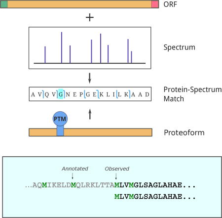
Graphical abstract
Introduction
Bottom-up proteogenomics is now a mature area that proved to be valuable for improving genome annotations in both prokaryotes1–5 and eukaryotes6–8. E.g., Kucharova and Wiker9 discussed over a hundred papers aimed at annotating various genomes in a recent review focusing on bacterial proteogenomics. However, previous proteogenomics studies focused on bottom-up mass spectrometry and have not utilized the power of top-down proteomics yet.
While bottom-up bacterial proteogenomics has been successful, prediction of short genes, annotation of genes with unusual codon usage, and accurate prediction of Start codons remains a challenge. Moreover, the capabilities of bottom-up proteogenomics for solving such challenging problems as annotating post-translational modifications (chemical modifications, signal peptides, proteolytic events) are limited because it provides only partial coverage of various proteoforms by short peptides.
In addition to proteogenomics, ribosome profiling (Ribo-seq) is another recently introduced approach to genome annotation that enabled the direct observation of protein synthesis at the transcript level. While Ribo-seq resulted in recent discoveries of elusive (often short) proteins forming a “hidden proteome”, it may generate false predictions10. Thus, it needs to be complemented by more reliable techniques for validating gene annotations11. Bottom-up proteogenomics is not an ideal way to validate Ribo-seq data since elusive short proteins in “hidden proteome” often lack identified peptides or are represented by less reliable “one-hit-wonders”.12 Top-down proteogenomics, on the other hand, provides a full-length protein coverage and can potentially identify the entire short protein if it is expressed at the detectable level.
We emphasize that bottom-up and top-down proteogenomics have unique strengths and limitations and thus represent complementary approaches. E.g., while top-down proteogenomics generates a full-length protein coverage, its applications are mainly limited to identification of relatively short proteins. Thus, ideally bottom-up and top-down approaches should be combined together13.
Below we describe SpectroGene software tool for top-down proteogenomics and benchmark it on a large set of top-down mass spectra from Salmonella Typhimurium.
Methods
Top-down protein identification
In this study, we used TopPIC14 for all protein identifications. TopPIC is a modification of MS-Align+15 with improved ability to characterize post-translational modifications. Similarly to other top-down database search tools, TopPIC has ability to identify proteoforms with large N- and C-terminal modifications as well as multiple modifications on internal residues. An important feature of TopPIC is the ability to generate accurate P-values and E-values of Protein-Spectrum Matches (PrSMs), a prerequisite for a reliable prediction of new genes.
TopPIC extends MS-Align+ by improved PTM localization in the found PrSMs, computing the confidence scores of the candidate PTM sites, and utilizing triplets of CID/HCD/ETD spectra for PrSM search. It also optimizes MS-Align+ in a variety of ways: (i) indexing protein databases to reduce the memory footprint in the MS/MS database search; (ii) improved filtering algorithm to increase the sensitivity of spectral identification; (iii) an improved spectral alignment algorithm allowing users to specify the range of unexpected mass shifts; (iv) a lookup table-based approach to speed up the computation of P-values and E-values of PrSMs16.
Forming ORFeome
The existing top-down tools ProsightPC17, MS-Align+15 and TopPIC14 were designed for finding PrSMs by searching all spectra against all annotated proteins in a proteome. When the proteome is unknown, we build an OR-Feome by breaking the six-frame translation of the genome into Open Reading Frames (ORFs). The Stop codons break the sequence of n/3 codons in each of frame of the n-nucleotide long genome into segments between every pair of consecutive Stop codons. The suffixes of these segments that begin at the first Start codon within a segment form ORFs. ORFs within a single genomic sequence may overlap because there are six possible reading frames.
Most spectra identified in this study can be found by a simple TopPIC search against all ORFs. However, we found that this simple search fails to identify some spectra resulting from short proteoforms within long ORFs. Such “lost” identifications are often caused by the heuristic filtration step in TopPIC that trades accuracy for speed15,18. Thus, to increase the number of identified spectra, we used the ORF splitting approach described below.
We divide all ORFs from six-frame translation into short (length does not exceed a predefined length threshold L) and long (length exceeds L). We further split long ORFs into overlapping windows of length L, such that the consecutive windows overlap by L/2 nucleotides (see Figure 1). Tiling long ORFs by the overlapping windows is important since otherwise there is a risk of missing PrSMs that span two consecutive windows.
Figure 1.

Generating the ORFeome. Start and Stop codons are shown in green and red, respectively. ORFs longer than L are partitioned into overlapping windows of length L to increase the sensitivity of PrSM identifications.
While ORF splitting addresses one of the limitations of TopPIC (identifications of a spectrum arising from a short proteoform within a long protein), TopPIC may also miss a proteoform spanning over multiple windows if the window length L is too short. To address this limitation of TopPIC, we generate the ORFeome for a range of window lengths. The default values of L are 50,200,500 (L = 500 represents the limit for the length proteins typically identified by top-down mass spectrometry). We note that other reasonable values of parameter L result in similar sets of identified spectra.
Identifying Protein-Spectrum Matches
Each spectrum may have multiple matches against the ORFeome for various window lengths L. We select a single match corresponding to a PrSM with the minimum P-value for a given spectrum. PrSMs with the E-values below a threshold are reported (0.01 is the default E-value threshold for SpectroGene). We refer to proteins/peptides that correspond to these PrSMs as proteoforms19. The E-value of a proteoform is defined as the minimum E-value of all PrSMs that correspond to this proteoform. See Figure 2a for a diagram illustrating the concept of a proteoform.
Figure 2.

A diagram illustrating the concepts of proteoforms and ORF clusters. Start and Stop codons are shown in green and red respectively.
Annotating genomes by proteoforms
SpectroGene combines identified proteoforms into ORF clusters in such a way that proteoforms from the same cluster belong to the same ORF in the six-frame translation of the genome. Note, that while proteoforms from the same ORF cluster belong to the same ORF, they do not necessarily cover the full length of the ORF. We define the first/last amino acid of the ORF cluster as the first/last amino acid across all its proteoforms. The length of the ORF cluster is defined as the number of amino acids between its first and last amino acids The ORF cluster is typically shorter than the corresponding ORF. See Figure 2b for a diagram illustrating the concept of the ORF cluster.
Software
SpectroGene is an easy-to-use open source software written in Python and freely available at http://github.com/fenderglass/SpectroGene. It takes as input (i) deconvoluted top-down spectra and (ii) genomic sequence and outputs the report describing the found proteoforms and ORF clusters. TopPIC is included into the distribution. Additionally, a user can provide a set of annotated proteins to perform conventional database search against a proteome.
Results
Datasets
We benchmarked SpectroGene on a large top-down spectral dataset from Salmonella Typhimurium strain LT2 containing 22,683 spectra13 and a small top-down spectral dataset from Pyrococcus furiosus containing 1,198 spectra20. Below we provide the detailed description of the benchmarking results for the large dataset and a brief description for the small dataset.
This large dataset was generated using single-dimension ultra–high-pressure liquid chromatography (UPLC) system coupled with a Velos-Orbitrap mass spectrometer to profile the intact S. Typhimurium proteome. S. Typhimurium genome (4,86 millions nucleotides in length) has 4,451 annotated proteins. 427 of them are relatively short proteins (shorter than 100 amino acids in length) that are often difficult to predict using existing software tools for bacterial gene prediction21,22. Proteome was downloaded from the UniProt database (accession number UP000001014, only chromosomal genes were considered).
The small dataset was generated using capillary electrophoresis (CE) through a sheathless capillary electrophoresis-electrospray ionization (CESI) interface coupled to an Orbitrap Elite mass spectrometer20. The Pyrococcus Furiosus proteome was down-loaded from the UniProt database (accession number UP000001013).
Comparison of SpectroGene with conventional protein database search
We first benchmarked SpectroGene against the conventional proteome database search. To make this comparison, we performed a SpectroGene run referred as a genome run (comparing all spectra against the genome) and a proteome run which is described as follows.
We first perform a conventional search against a known proteome using TopPIC with the same parameters as in the genome run. Then we project the found proteoforms on the genome by aligning their amino acid sequences on the genomic sequence using BLAST. ORF clusters of the proteome run are defined in the same way as in the genome run.
SpectroGene identified 2,665 proteoforms from 599 distinct ORF clusters in the genome run, while TopPIC identified 2,600 proteoforms from 598 distinct ORF clusters in the proteome run. Figure 3 shows the distribution of lengths of identified proteoforms, ORF clusters, and ORFs in the genome run. ORF clusters that were identified by SpectroGene cover 584 out of 598 (97%) ORF clusters identified in the proteome run. The fact that nearly all ORF clusters identified in the proteome run were also identified in the genome run underscores the potential of top-down proteomics for genome annotation.
Figure 3.

The distribution of lengths of proteoforms (a), ORF clusters (b), and ORFs (c) identified in the genome run. The increased proportion of longer ORF clusters comparing to the median proteoform length is explained by the fact that some long proteins give rise to multiple short proteoforms. One ORF cluster and six ORFs with lengths exceeding 1000 aa are not shown.
A slightly larger number of proteoforms/ORF clusters identified in the genome run does not imply that the genome runs are superior to the proteome runs but is rather an indication that there are fewer constraints in identifying the endpoints of putative proteoform when the proteome is unknown Liu et al.15. In some cases, these endpoints are not true ends of proteoforms but rather computational artifacts since all top-down tools are prone to errors in the case of large modifications and errors in estimating the precursor masses.
Next, we assess how accurate SpectroGene is with respect to identification of specific gene features, e.g., translational start sites (referred to as gene starts) or signal peptides. We refer to an ORF cluster as the gene end if it ends right before the Stop codon. We refer to an ORF cluster as a potential gene start if either (i) its first codon is a Start codon (ATG, GTG, or TTG) or (ii) its preceding codon is a Start codon and its first amino acid is Gly, Ala, Ser, Cys, Thr, Pro, or Val. The condition (ii) accounts for N-terminal Methionine Cleavage (NME) that removes the initial methionine from proteins whose second residue is Gly, Ala, Ser, Cys, Thr, Pro, or Val23. We say that an ORF cluster reveals a potential signal peptide if its start precedes by the canonical signal peptide recognition motif A.A. Since the recognition sites for many signal peptides often deviate from the canonical A.A motif, we also specify a weaker test for the signal peptide motif that is limited to a single amino acid A at position −1. This rule results in a higher false positive but smaller false negative rates for the signal peptide detection. For each weak and strong signal peptide motif we measured the distance from a cut to the annotated gene start. The median value was equal to 22, which lies in the expected range for the length of signal peptides.
The statistics of ORF clusters corresponding to gene starts/ends (as well as potential signal peptides) for both genome and proteome runs are given in Table 1. As expected, many proteins are only partially covered by corresponding proteoforms. As the result, many ORF clusters do not begin with a Start codon or end with a Stop codon. However, there is a good agreement between the genome and the proteome searches with respect to the number of identified gene starts and ends.
Table 1.
Statistics of ORF clusters identified in the proteome run and in the genome runs.
| Statistics | Proteome run | Genome run |
|---|---|---|
| #PrSMs | 8539 | 8368 |
| #proteoforms | 2600 | 2665 |
| #ORF clusters | 598 | 599 |
| Median ORF cluster length | 99 | 99 |
| Gene start | 175 (29%) | 169 (28%) |
| Gene end | 329 (55%) | 326 (54%) |
| Gene start AND gene end | 183 (30%) | 172 (28%) |
| Neither gene start nor gene end | 205 (34%) | 210 (35%) |
| Precedes by the canonical signal peptide motif A.A | 30 (5%) | 31 (5%) |
| Precedes by the weak signal peptide motif A | 79 (13%) | 78 (13%) |
Using SpectroGene to find new genes
Next, we analyze the differences between genome and proteome runs as the specific ORF clusters (identified in the genome run but not in the proteome run) may potentially represent genes that are currently not annotated.
Interestingly, most of the specific ORF clusters (that were identified in the genome run but not in the proteome run and vice versa) have significantly higher E-values than the average E-values of identified proteoforms (Figure 4). It is expected that, due to the larger search space, most proteoforms identified in the genome run have higher E-values than proteoforms identified in the proteome run. However, in some cases, proteoforms might have higher E-value in the proteome comparing to the genome run (see the section below for comparing the E-values of proteoforms identified in proteome and genome searches).
Figure 4.

Histogram of log-scaled E-values of ORF clusters found in genome/proteome run that have (blue) or do not have (red and green) a “matching” ORF cluster in proteome/genome run respectively. E-value of an ORF cluster is defined as the lowest E-value among all proteoforms that belong to this ORF cluster. While most of ORF clusters without match have higher E-values than the median E-value of all identified proteoforms, a few ORF clusters have relatively low E-values. These ORF clusters reveal previously unannotated genes or represent paralogous gene copies.
14 ORF clusters identified in the proteome run were not identified in the genome run (proteoforms mapping to these ORF clusters have E-values varying from 10−2 to 10−10). Eight of them were identified by SpectroGene but were not reported because they had E-values slightly above the threshold. Other six clusters either represent paralogous copies of the genes identified in the genome run or erroneous hits.
15 ORF clusters were identified in the genome run but not in the proteome run. Six of them were found in the proteome run but were not reported since they had E-values slightly exceeding the threshold. For the remaining nine ORF clusters, we performed BLAST searches against the NCBI protein database. A BLAST hit of an ORF cluster against an annotated protein in another species represents a comparative genomics support for the hypothesis that the ORF cluster belongs to a yet unannotated gene in S. Typhimurium.
Seven out of nine ORF clusters had various statistically significant BLAST matches to annotated proteins in other bacteria thus suggesting that SpectroGene may complement the existing gene prediction tools. Figure 5 presents examples of two PrSMs from such ORF clusters with the lowest E-values (10−17 and 10−30) revealing potentially new genes in S. Typhimurium. For the remaining two out of nine of ORF clusters (without statistically significant BLAST hits), the proteoforms mapping to these ORF clusters had relatively high E-values (≈ 10−3). Thus, since we only have a borderline statistical evidence that these ORF clusters reveal new genes, we view them as potential false positives.
Figure 5.

MS-Align+ logos of PrSMs. Symbols in bold represent proteoforms with red brackets on its ends, while gray symbols show flanking genomic sequence between two consecutive stop codons. Symbols
 and
and
 refer to the b- and y- ions. Symbol
 refere to the case when both b- and y-ions are present in the spectrum. Putative Start codons are shown in green. Stop codons are indicated by “*” signs. Blue background marks a possible location of the PTM with the mass shift −2.01 shown on top. Since TopPIC is unable to place this PTM on a specific residue, it assigns it to one of the six residues shown in the blue background.
The proteoform shown in Figure 5(a) represents a short protein with unusually high fraction (45%) of proline residues. Such proline-rich proteins (PRPs) have been reported in various bacteria. While the function of most such proteins remains unclear, some of them have been implicated in signal transduction24. The proteolytic pathway that resulted in this 31 amino acids long proteoform remains unknown.
The proteoform shown in Figure 5(b) represents a short (59 amino acids) protein with −2 Da modification that suggests the disulfide bridge between two cysteins separated by seven amino acids. Since this proteoform starts at the first Methionine in an ORF and ends right before the Stop codon, it covers the entire gene.
Interestingly, the ORF clusters identified in the genome run contain 119 out of 427 (≈ 28%) proteins shorter than 100 amino acids in S. Typhimurium. This result indicates that top-down proteomics provides excellent coverage of the short proteome that is traditionally difficult to predict using existing gene prediction tools or validate using traditional bottom-up proteomics approaches. Indeed, the number of short proteins identified using our small top-down dataset exceeds the number of short proteins identified using a large bottom-up bacterial dataset in Gupta et al.4 by an order of magnitude.
Using SpectroGene to improve gene annotations
Top-down proteogenomics has a potential to improve existing gene annotations by correcting missannotated gene starts. From the 169 ORF clusters identified in the genome run that were marked as gene starts, 139 show agreement with existing gene annotations. For the remaining 30 ORF clusters we observe a systematic shift of Start codons reported by SpectroGene to the right (with a median value of 16). Most of these shifts correspond to genes that are only partially covered by proteoforms. These proteoforms most likely correspond to proteolytically digested proteins, e.g., three of them start at the likely position of the signal peptide cleavage. However, we observe two interesting examples of alternative gene starts, which do not agree with proteome annotations and are also unlikely to be caused by proteolytic events (see Figure 6).
Figure 6.

Examples of gene start corrections using identified proteoforms. Putative Start codons are marked in green. Since the observed gene starts are located after the annotated gene starts, the gene start corrections in these examples can be made based on both genome and proteome runs.
Benchmarking SpectroGene using Pyrococcus furiosus dataset
SpectroGene identified 186 proteoforms from 91 distinct ORF clusters in the genome run and 178 proteoforms from 87 ORF clusters in the proteome run. 4 out of the 87 ORF clusters identified the proteome run did not overlap with proteins identified using ProsightPC in the original study20.
One ORF cluster from the proteome run was not identified in the genome run because its E-value slightly exceeded the threshold. We also observe five ORF clusters (with E-values from 10−4 to 10−36) from the genome run that were missed in the proteome suggesting gaps in the proteome annotations. Four out of these five ORF clusters represent proteins that were not annotated in the proteome. Figure 7 illustrates the PrSM diagrams for two out of four ORF clusters specific to the genome run.
Figure 7.

MS-Align+ logos of PrSMs found in P. furosus genome that are not annotated in the proteome. All PrSMs have statistically significant BLAST hits against (identical) computationally predicted hypothetical proteins in P. furiosus.
Interestingly, one of the five ORF clusters specific to the genome was not identified in the proteome run due to an apparent error in predicting the gene start for this ORF cluster (see Figure 8 for details). We observed 2 more discrepancies between the annotated and observed gene starts in P. furiosus.
Figure 8.

A proteoform representing the Iron-dependent repressor of P. furiosus reveals the likely error in the gene start annotation. As a consequence, this proteoform was not identified in the proteome run.
SpectroGene performance
We benchmarked the running time and memory footprint of SpectroGene for both genome and proteome runs (see Table 2). The most time-consuming step of the algorithm is PrSM identification with TopPIC. However, this step could be done in parallel, which gives a significant speed-up.
Table 2.
Speed and memory usage statistics of SpectroGene. Benchmarks were performed on S. Typhimurium and P.Furiosus datasets. SpectroGene was run in parallel on a cluster with 20 Intel Xenon cores.
| S. Typhimurium | P. Furiosus | |||
|---|---|---|---|---|
| Proteome | Genome | Proteome | Genome | |
| Database size (Mb) | 1.5 | 10 | 0.8 | 3.7 |
| Number of spectra | 22, 638 | 22, 638 | 1, 221 | 1, 198 |
| Running time (min) | 2307 | 4784 | 74 | 164 |
| Memory usage (Gb) | 76 | 76 | 76 | 76 |
To assess how E-values reported by SpectroGene correlate with false discovery rate (FDR) of SpectroGene searches, we used a variation of the target-decoy approach25 and randomly shuffled all sequences in both genome and proteome runs to generate the decoy database. We then calculated FDR as the ratio of the number of PrSMs found in the resulting decoy runs and the number of proteoforms in the found in the SpectroGene with the target database. The FDR was the proteome and the genome runs was estimated at 1.2% and 1.1%, respectively. Thus, the computed FDR correlates well with the E-value threshold 0.01 used for both runs.
Comparing E-values of PrSMs in genome and proteome searches
Since the size of the genome database is larger than the size of the proteome database, we expect that E-values of PrSMs in the genome run are larger than E-values of PrSMs in the proteome run. However, E-values in top-down searches are defined by both database size and p-values of PrSMs. Since computing exact p-values of PrSMs remains an open problem (Liu et al.15 only described an exact formula for the case of PrSMs formed by proteoforms without N- and C-terminal modifications), TopPIC approximates p-values using a heuristic approach. Since p-values of PrSMs in proteome searches may be larger than p-values of PrSMs in genome searches, E-values of some PrSMs in proteome searches are slightly larger than E-values of these PrSMs in genome searches.
Discussion
In recent years, proteogenomics has become especially relevant in microbiology where over 30,000 bacterial genomes have been sequenced and where the limitations of existing gene prediction tools are well recognized. For example, a comparison of various state-of-the-art gene prediction tools for the sequences of Mycobacterium tuberculosis H37Rv and Halorhabdus utahensis showed up to 50% difference in the Start codon assignments26,27. In some bacterial genomes, these tools incorrectly assign nearly 60% of Start codons28.
The idea of searching tandem mass spectra against the translated genome (rather than derived proteome) in order to validate the existing annotation was introduced by Jaffe et al.29 and resulted in many bottom-up proteogenomics studies in the last decade. However, as Kucharova and Wiker9 noted in a recent review, bottom-up proteogenomics studies suffer from the rather low protein sequence coverage by peptides.
Top-down mass spectrometry has advantages in localizing multiple PTMs in a coordinated fashion and identifying multiple protein species (e.g. proteolytically processed protein species). In the last five years, because of advances in protein separation and top-down instrumentation, top-down mass spectrometry moved from analyzing single proteins to analyzing complex samples containing hundreds and even thousands of proteins thus opening new opportunities for proteogenomics annotations. However, computational tools for top-down proteogenomics are still missing.
In some applications, top-down proteogenomics clearly has advantages over bottom-up proteogenomics. For example, Bonissone et al.23 recently conducted a large bottom-up proteogenomics study of N-terminal protein processing by analyzing 112 million spectra from 57 bacterial organisms. However, bottom-up analysis of N-terminal processing of a given protein only succeeds if the N-terminal peptide in this protein is identified, the condition that holds only for a fraction of proteins identified in Bonissone et al.23. While various techniques for enrichment of N-terminal peptides have been used to improve start site annotations30,31, they are still rarely used in proteogenomics studies since they remain error prone and require additional experimental protocols. Top-down proteogenomics, on the other hand, identifies intact proteins and thus provides information on N-terminus of every identified proteoform.
All previous proteogenomics studies were based on bottom up mass spectrometry with the only exception is Ansong et al.13 that however has not resulted in a publicly available software tool for top-down proteogenomics. This study introduced SpectroGene, the first such tool that has a potential to be used in conjunction with each proteogenomics study of bacterial genomes. We have shown that, using unannotated genome, SpectroGene generates results that are in a good agreement with the state-of-the-art protein identification tools that use annotated genome, i.e., the protein database. We also identified some putative proteins that were missed by the search against the proteome database.
Acknowledgments
We thank Aaron Aslanian and John Yates for providing top-down spectra for Pyrococcus furiosus. MK and PAP are supported by National Institute of Health (grant 5P41GM103484). PAP has an equity interest in Digital Proteomics, LLC, a company that may potentially benefit from the research results.
Footnotes
The terms of this arrangement have been reviewed and approved by the University of California, San Diego in accordance with its conflict of interest policies.
References
- 1.Yates Jr, Eng J, McCormack A. Mining genomes: correlating tandem mass spectra of modified and unmodified peptides to sequences in nucleotide databases. Anal. Chem. 1995;67:3202–3202. doi: 10.1021/ac00114a016. [DOI] [PubMed] [Google Scholar]
- 2.Jaffe H, Vinade L, Dosemeci A. Identification of novel phosphorylation sites on postsynaptic density proteins. Biochem. Biophys. Res. Commun. 2004;321:210–218. doi: 10.1016/j.bbrc.2004.06.122. [DOI] [PubMed] [Google Scholar]
- 3.Fermin D, Allen BB, Blackwell TW, Menon R, Adamski M, Xu Y, Ulintz P, Omenn GS, States DJ. Novel gene and gene model detection using a whole genome open reading frame analysis in proteomics. Genome Biol. 2006;7:R35. doi: 10.1186/gb-2006-7-4-r35. [DOI] [PMC free article] [PubMed] [Google Scholar]
- 4.Gupta N, Tanner S, Jaitly N, Adkins JN, Lipton M, Edwards R, Romine M, Osterman A, Bafna RD, Smith Vineet amd, Pevzner PA. Whole proteome analysis of post-translational modifications: applications of mass-spectrometry for proteogenomic annotation. Genome Res. 2007;17:1362–1377. doi: 10.1101/gr.6427907. [DOI] [PMC free article] [PubMed] [Google Scholar]
- 5.Gupta N, Benhamida J, Bhargava V, Goodman D, Kain E, Kerman I, Nguyen N, Ollikainen N, Rodriguez J, Wang J, Lipton MS, Romine M, Bafna V, Smith RD, Pevzner PA. Comparative proteogenomics: combining mass spectrometry and comparative genomics to analyze multiple genomes. Genome Res. 2008;18:1133–1142. doi: 10.1101/gr.074344.107. [DOI] [PMC free article] [PubMed] [Google Scholar]
- 6.Castellana NE, Payne SH, Shen Z, Stanke M, Bafna V, Briggsc SP. Discovery and revision of Arabidopsis genes by proteogenomics. PNAS. 2008;18:21034–21038. doi: 10.1073/pnas.0811066106. [DOI] [PMC free article] [PubMed] [Google Scholar]
- 7.Woo S, Cha SW, Na S, Guest C, Liu T, Smith RD, Rodland KD, Payne SP, Bafna V. Proteogenomic strategies for identification of aberrant cancer peptides using large-scale next-generation sequencing data. Proteomics. 2014;14:2719–2730. doi: 10.1002/pmic.201400206. [DOI] [PMC free article] [PubMed] [Google Scholar]
- 8.Li H, Menon R, Omenn G, Guan Y. Revisiting the identification of canonical splice isoforms through integration of functional genomics and proteomics evidence. Proteomics. 2014;14:2709–2718. doi: 10.1002/pmic.201400170. [DOI] [PMC free article] [PubMed] [Google Scholar]
- 9.Kucharova V, Wiker HG. Proteogenomics in microbiology: Taking the right turn at the junction of genomics and proteomics. Proteomics. 2014;14:2660–2675. doi: 10.1002/pmic.201400168. [DOI] [PubMed] [Google Scholar]
- 10.Stern-Ginossar N, Weisburd B, Michalski A, Le VTK, Hein MY, Huang S-X, Ma M, Shen B, Qian S-B, Hengel H, Mann M, Ingolia NT, Weissman JS. Decoding Human Cytomegalovirus. Science. 2012;338:1088–1093. doi: 10.1126/science.1227919. [DOI] [PMC free article] [PubMed] [Google Scholar]
- 11.Koch A, Gawron D, Steyaert S, Ndah E, Crappé J, De Keulenaer S, De Meester E, Ma M, Shen B, Gevaert K, Criekinge WV, Van Damme P, Menschaert G. A proteogenomics approach integrating proteomics and ribosome profiling increases the efficiency of protein identification and enables the discovery of alternative translation start sites. Proteomics. 2014;14:2688–2689. doi: 10.1002/pmic.201400180. [DOI] [PMC free article] [PubMed] [Google Scholar]
- 12.Veenstra TD, Conrads TP, Issaq HJ. What to do with “one-hit wonders”. Electrophoresis. 2004;25:1278–1279. doi: 10.1002/elps.200490007. [DOI] [PubMed] [Google Scholar]
- 13.Ansong C, Wu S, Da M, Liu X, Brewer HM, Deatherage Kaiser BL, Nakayasu ES, Cort JR, Pevzner P, Smith RD, Heffron F, Adkins JN, Paša-Tolić L. Top-down proteomics reveals a unique protein S-thiolation switch in Salmonella Typhimurium in response to infection-like conditions. PNAS. 2013;110:10153–10158. doi: 10.1073/pnas.1221210110. [DOI] [PMC free article] [PubMed] [Google Scholar]
- 14.TopPIC. website: http://proteomics.informatics.iupui.edu/software/toppic/index.html.
- 15.Liu X, Sirotkin Y, Shen Y, Anderson G, Tsai YS, Ting YS, Goodlett DR, Smith RD, Bafna V, Pevzner PA. Protein identification using top-down spectra. Mol. Cell. Proteomics. 2011;13:2752–2764. doi: 10.1074/mcp.M111.008524. [DOI] [PMC free article] [PubMed] [Google Scholar]
- 16.Liu X, Segar MW, Li SC, Kim S. Spectral probabilities of top-down tandem mass spectra. BMC genomics. 2014;15:S9. doi: 10.1186/1471-2164-15-S1-S9. [DOI] [PMC free article] [PubMed] [Google Scholar]
- 17.Zamdborg L, LeDuc RD, Glowacz KJ, Kim Y-B, Viswanathan V, Spaulding IT, Early BP, Bluhm EJ, Babai S, Kelleher NL. ProSight PTM 2.0: improved protein identification and characterization for top down mass spectrometry. Nucleic Acids Res. 2007;35:W701–W706. doi: 10.1093/nar/gkm371. [DOI] [PMC free article] [PubMed] [Google Scholar]
- 18.Liu X, Mammana A, Bafna V. Speeding up tandem mass spectral identification using indexes. Bioinformatics. 2012;28:1692–1697. doi: 10.1093/bioinformatics/bts244. [DOI] [PMC free article] [PubMed] [Google Scholar]
- 19.Smith LD, Kelleher NL. The Consortium for Top Down Proteomics, Proteoform: a single term describing protein complexity. Nat. Methods. 2013;10:186–187. doi: 10.1038/nmeth.2369. [DOI] [PMC free article] [PubMed] [Google Scholar]
- 20.Han X, Wang Y, Aslanian A, Bern M, Lavallée-Adam M, III, J RY. Sheathless Capillary Electrophoresis-Tandem Mass Spectrometry for Top-Down Characterization of Pyrococcus furiosus Proteins on a Proteome Scale. Anal. Chem. 2014;86:11006–11012. doi: 10.1021/ac503439n. [DOI] [PMC free article] [PubMed] [Google Scholar]
- 21.Borodovsky M, McIninch J. GENMARK: Parallel gene recognition for both DNA strands. Comput. Chem. 1993;17:123–133. [Google Scholar]
- 22.Salzberg SL, Delcher AL, Kasif S, White O. Microbial gene identification using interpolated Markov models. Nucleic Acids Res. 1998;26:544–548. doi: 10.1093/nar/26.2.544. [DOI] [PMC free article] [PubMed] [Google Scholar]
- 23.Bonissone S, Gupta N, Romine M, Bradshaw RA, Pevzner PA. N-terminal Protein Processing: A Comparative Proteogenomic Analysis. Mol. Cell. Proteomics. 2013;12:14–28. doi: 10.1074/mcp.M112.019075. [DOI] [PMC free article] [PubMed] [Google Scholar]
- 24.Williamson MP. The structure and function of proline-rich regions in proteins. Biochem. 1994;297:249–260. doi: 10.1042/bj2970249. [DOI] [PMC free article] [PubMed] [Google Scholar]
- 25.Elias JE, Gygi SP. Target-Decoy Search Strategy for Mass Spectrometry-Based Proteomics. Methods Mol. Biol. 2010;604:55–77. doi: 10.1007/978-1-60761-444-9_5. [DOI] [PMC free article] [PubMed] [Google Scholar]
- 26.de Souza GA, Målen H, Søfteland T, Sælensminde G, Prasad S, Jonassen I, Wiker HG. High accuracy mass spectrometry analysis as a tool to verify and improve gene annotation using Mycobacterium tuberculosis as an example. BMC Genomics. 2008;9:316. doi: 10.1186/1471-2164-9-316. [DOI] [PMC free article] [PubMed] [Google Scholar]
- 27.Bakke P, Carney N, DeLoache W, Gearing M, Ingvorsen K, Lotz M, McNair J, Penumetcha P, Simpson S, Voss L, Win M, Heyer LJ, Campbell AM. Evaluation of Three Automated Genome Annotations for Halorhabdus utahensis. PLOS One. 2009;4:e6291. doi: 10.1371/journal.pone.0006291. [DOI] [PMC free article] [PubMed] [Google Scholar]
- 28.Nielsen P, Krogh A. Large-scale prokaryotic gene prediction and comparison to genome annotation. Bioinformatics. 2005;21:4322–4329. doi: 10.1093/bioinformatics/bti701. [DOI] [PubMed] [Google Scholar]
- 29.Jaffe JD, Berg HC, Church GM. Proteogenomic mapping as a complementary method to perform genome annotation. Proteomics. 2004;4:59–77. doi: 10.1002/pmic.200300511. [DOI] [PubMed] [Google Scholar]
- 30.Jaffe JD, Berg HC, Church GM. N-Terminal-oriented Proteogenomics of the Marine Bacterium Roseobacter Denitrificans Och114 using N-Succinimidyloxycarbonylmethyl)tris(2,4,6-trimethoxyphenyl)phosphonium bromide (TMPP) Labeling and Diagonal Chromatography. Mol. Cell. Proteomics. 2014;13:1369–1381. doi: 10.1074/mcp.O113.032854. [DOI] [PMC free article] [PubMed] [Google Scholar]
- 31.Bertaccini D, Vaca S, Carapito C, Arsène-Ploetze F, Dorsselaer AV, Schaeffer-Reiss C. An improved stable isotope N-terminal labeling approach with light/heavy TMPP to automate proteogenomics data validation: dN-TOP. J. Proteome Res. 2013;12:3063–3070. doi: 10.1021/pr4002993. [DOI] [PubMed] [Google Scholar]