Sparse canonical correlation analysis between an alcohol biomarker and self-reported alcohol consumption

Abstract

In investigating the correlation between an alcohol biomarker and self-report, we developed a method to estimate the canonical correlation between two high-dimensional random vectors with a small sample size. In reviewing the relevant literature, we found that our method is somewhat similar to an existing method, but that the existing method has been criticized as lacking theoretical grounding in comparison with an alternative approach. We provide theoretical and empirical grounding for our method, and we customize it for our application to produce a novel method, which selects linear combinations that are step functions with a sparse number of steps.

1. Motivating study

The WHAT-IF clinical trial is a randomized comparison of naltrexone versus placebo that was designed to determine whether naltrexone can reduce hazardous drinking in women living with HIV. The protocol is registered with clinicaltrials.gov as NCT01625091, and it can be found at https://clinicaltrials.gov/ct2/show/NCT01625091. Alcohol consumption is measured via self-report and the biomarker PEth. Our colleagues are interested not only in determining the effect of naltrexone, but also in measuring the correlation between the two measures of consumption. Previous studies have indicated that PEth is well correlated with alcohol intake and has a detection window of 1 to 3 weeks following back such as Aradottir et al. (2006), Stewart et al. (2009), Hahn et al. (2012), Helander et al. (2012), Viel et al. (2012), Jain et al. (2014), and Kechagias et al. (2015). Standard drink units (SDUs) are typically used to quantify alcohol consumption; one SDU corresponds to 0.6 ounces of pure alcohol, which is approximately one 12 ounce 5% alcohol by volume (ABV) beer, one 5 ounce glass of wine, or 1.5 ounces of a 40% ABV spirit. The WHAT-IF clinical trial included women who reported hazardous drinking (>7 SDUs per week) at baseline. Self-reported daily alcohol consumption was recorded from 90 days prior to baseline through 7 months after baseline using timeline followback, a detailed interview that uses a calendar and example glassware to maximize reporting accuracy. PEth was measured at baseline, 2 months, 4 months, and 7 months. Some study participants were missing one or more PEth measurements, and a few others reported implausible alcohol consumption. We excluded individuals who ever reported consuming more than 50 SDUs in 1 day, resulting in a final sample of 114 women.

Canonical correlation analysis (CCA) is widely used to assess the association between two sets of variables, and to identify a linear combination of variables (a composite measure) from each set such that the correlation between the two composite measures is maximized (Mardia et al., 1979). However, when the ratio of the number of variables to the sample size is high, the results based on the classical CCA break down in the sense that the estimated linear combinations and resulting correlation can be very far from the truth. This article presents a case study focusing on estimating the correlation between a single PEth measurement and 21 previous days of self-reported SDUs, while accounting for repeated PEth measures per person. Because the correlation between PEth and daily alcohol consumption is expected to decrease with the time since previous drinking, we assume that the coefficients of the linear combination of daily alcohol consumption can be represented by a step function that jumps at the time or times when the correlation decreases. Due to the curse-of-dimensionality problem arising from a large number of daily SDUs and a relatively small number of women, we need to restrict the number of jumps of our step function in some way or else the result will be so noisy as to be useless. To do so, we use an L¹ penalty on the coefficients of a non-orthogonal set of step function basis functions. Based on our literature search, using the Lasso in combination with the step function basis is a simple yet novel way to achieve our goal.

Because higher body mass index is likely to be associated with higher self-reported consumption and also with PEth biomarker results, we also consider a partial canonical correlation analysis, in which we remove the effect of body mass index.

As is often the case within applied statistics, we developed our method to answer our collaborators’ question, and then only afterward did we search the literature to compare our method to existing methods. The plan of the article is as follows. In Section 2, we review the literature on existing methods for estimating a canonical correlation that circumvent the curse of dimensionality. Section 3 then presents our own method for estimating a sparse canonical correlation between two sets of measures. We compare our method to that of Waaijenborg et al. (2008), which is the only method we found that is somewhat similar to ours. However, there is a key difference that leads to much faster convergence of our method in general. Our use of the step function basis in conjunction with the Lasso is also new. We conduct a simulation study in Section 4, and we apply our methods to the WHAT-IF trial in Section 5. Section 6 concludes with a discussion.

2. Review of existing methods

Let y and x be two vectors representing the sets of variables to be correlated. Classical canonical correlation analysis (CCA) selects the α and β that maximize the correlation

$$\rho ({\mathbf{y}}^T\alpha ,{\mathbf{x}}^T\beta )=\frac{{\beta }^T\text{Cov}(\mathbf{x},\mathbf{y})\alpha }{\sqrt{{\alpha }^T\text{Var}(\mathbf{y})\alpha {\beta }^T\text{Var}(\mathbf{x})\beta }}.$$ (2.1)

Because (2.1) does not depend on the scaling of α and β but rather just on their directions, we can view the problem as one of finding the two directions that maximize the correlation. Typically, one chooses the default scaling α^TVar(y)α = β^TVar(x)β = 1. The optimization problem then is to maximize the numerator of (2.1) subject to the constraints α^TVar(y)α = β^TVar(x)β = 1.

To overcome the curse of dimensionality arising from small samples and high-dimensional x or y, some researchers such as Vinod (1976), Leurgans et al. (1993), and Silverman and Ramsay (2005) proposed regularized canonical correlation analysis (RCCA) by modifying the constraints with penalties on α and β. For example, Vinod (1976) imposed ridge regression constraints α^T (Var(y) + λ₂I)α = β^T (Var(x) + λ₁I)β = 1, which would shrink the components of α and β toward zero for larger values of λ₁ and λ₂. Leurgans et al. (1993) imposed smoothing constraints α^T (Var(y) + λ₂D₂)α = β^T (Var(x) + λ₁D₁)β = 1 for D₁ and D₂ selected to shrink α and β toward smooth functions for larger λ₁ and λ₂. Once a suitable quadratic penalty is found, the optimization problem is readily solved in the same way it is for classical CCA.

Other researchers such as Parkhomenko et al. (2007), Waaijenborg et al. (2008), Wiesel et al. (2008), Zhou and He (2008), Parkhomenko et al. (2009), Witten et al. (2009), and Witten and Tibshirani (2009) focused on providing sparse versions of α and β, which contain zeroes so that only a small subset of components of y and x are selected. These methods achieve what we term sparse canonical correlation analysis (SCCA). It is natural to consider an L¹, or Least Absolute Shrinkage and Selection Operator (Lasso) (Tibshirani, 1996), penalty with RCCA, but the resulting constraints are not quadratic which means that solving the optimization problem is difficult. We therefore considered using an iterated version of RCCA using an idea from Tibshirani (1996), in which we expressed the penalized constraints as ${\alpha }^T(\text{Var}(\mathbf{y})+{\lambda }_2{D}_b^{-})\alpha ={\beta }^T(\text{Var}(\mathbf{x})+{\lambda }_1{D}_a^{-})\beta =1$, where D_a and D_b are diagonal matrices with elements |α_i| and |β_j|, and $D_a^{-}$ and $D_b^{-}$ are their generalized inverses. This can be viewed as a “poorman’s” approach to solving the optimization problem of maximizing the numerator of (2.1) with non-quadratic L¹-penalty constraints α^TVar(y)α + λ₂||α||₁ = β^TVar(x)β + λ₁||β||₁ = 1. Unfortunately, the iterative algorithm often failed to converge, rendering this idea useless. The existing methods using non-quadratic penalties such as nonnegative Garrote (Breiman, 1995), Smoothly Clipped Absolute Deviation (SCAD; Fan and Li, 2001), Elastic-net (Zou and Hastie, 2005), and Lasso (Tibshirani, 1996) to produce sparse versions of α and β all simplify the optimization problem somehow. For example, Witten et al. (2009) and Witten and Tibshirani (2009) effectively assume that Var(x) and Var(y) are multiples of the identity, and the authors do not maximize a well-defined objective function. The authors set out to maximize β^TCov(x, y)α subject to α^Tα = 1, β^Tβ = 1, ||α||₁ ≤ c₁, and ||β||₁ ≤ c₂. However, for small c₁ and c₂, the constraints exclude all possible solutions. The authors therefore iteratively select c₁ and c₂ using cross-validation at each step of an iterative algorithm. This means that the optimization problem is changing with each iteration, because the constraints are changing. This problem is not mentioned in the articles.

The method we developed falls into the class of SCCA methods, and in implementation it is very similar to that of Waaijenborg et al. (2008). Witten and Tibshirani (2009) point out that the method of Waaijenborg et al. does not seem to be solving a well-defined optimization problem. For a scalar y and vector x, we construct a clearly posed optimization problem for our method, and for that special case, our method coincides with that of Waaijenborg et al. (2008); therefore in that case, Waaijenborg et al. are also solving a well-defined optimization problem. The value of studying the case of scalar y is the easy extension to the vector case; when y is a vector, we construct an optimization problem similar to but more general than that of Witten and Tibshirani (2009), and like those authors, we allow our constraints to change at each iteration. Our method is easy to implement using the glmnet package in R. We will explain the method of Waaijenborg et al. (2008) together with our method in the following section.

3. Sparse canonical correlation analysis

3.1. Sparse canonical correlation analysis between one random variable and one random vector

Let y, x₁, …, x_p be random variables such that E(y²) < ∞, $E(x_j^2)<\infty$ for j = 1, …, p. Define vector x = (x₁, …, x_p) as a 1 × p vector, and assume that the variance matrix of x is nonsingular. Then we can always write

$$y={\beta }_0+{\mathbf{x}}^{\mathbf{T}}\beta +\epsilon ,$$ (3.1)

where E(ε) = 0, E(ε²) < ∞, and Cov(x_j, ε) = 0 for j = 1, …, p (Wooldridge, 2010). Supposing β_C is a vector that maximizes the correlation ρ(y, x^Tβ), then λβ_C also maximize the correlation for any scalar λ. To motivate our method, we present the following simple results for scalar y. The results will be used to justify the iterative algorithm that we propose when y is a vector.

Theorem 3.1

Let y be a random variable and x be a vector of random variables such that Var(x) is nonsingular and Var(y) < ∞. Consider the following optimization solutions, where β₀ = E(y) − E(x^T)β:

$${\beta }^{\ast }={\mathit{argmin}}_{\beta }E{(y-{\beta }_0-{\mathbf{x}}^T\beta )}^2$$ (3.2)

and

$${\beta }_C={\mathit{argmax}}_{\beta }\rho (y,{\mathbf{x}}^T\beta )\mathit{subject}to{\beta }^T\mathit{Var}(\mathbf{x})\beta ={\beta }^{\ast T}\mathit{Var}(\mathbf{x}){\beta }^{\ast }.$$ (3.3)

Then β^* = β_C.

The theorem’s proof is given in the Appendix. We can also extend this result to the case of singular Var(x), which is relevant to the case of very high-dimensional x. In the Appendix, we show that the set of β^* that minimize (3.2) is identical to the set of β_C that maximize (3.3), and that ${\beta }^{\ast T}\text{Var}(\mathbf{x}){\beta }^{\ast }={\beta }_C^T\text{Var}(\mathbf{x}){\beta }_C$ is constant over that set.

When the ratio of the dimension of x to the sample size is high, we would like to choose a sparse β. One classic method is to introduce an L¹ constraint. Problems (3.2) and (3.3) become

$${\beta }_L={\text{argmin}}_{\beta }E{(y-{\beta }_0-{\mathbf{x}}^T\beta )}^2\text{subject}\text{to}{\Vert \beta \Vert }_1\le t$$ (3.4)

and

$${\beta }_C={\text{argmax}}_{\beta }\rho (y,{\mathbf{x}}^T\beta )\text{subject}\text{to}{\beta }^T\text{Var}(\mathbf{x})\beta ={{\beta }_L}^T\text{Var}(\mathbf{x}){\beta }_L,{\Vert \beta \Vert }_1\le t,$$ (3.5)

where with the equality constraint, $\rho (y,{\mathbf{x}}^T\beta )=\frac{{\beta }^T\text{Cov}(\mathbf{x},y)}{\sqrt{\text{Var}(y){\beta }^T\text{Var}(\mathbf{x})\beta }}=\frac{{\beta }^T\text{Cov}(\mathbf{x},y)}{\sqrt{\text{Var}(y){{\beta }_L}^T\text{Var}(\mathbf{x}){\beta }_L}}$. Let $a=\frac{\text{Cov}(\mathbf{x},y)}{\sqrt{\text{Var}(y){{\beta }_L}^T\text{Var}(\mathbf{x}){\beta }_L}}$. The problem (3.5) is

$${\beta }_C={\text{argmax}}_{\beta }{\beta }^{T}a\text{subject}\text{to}{\beta }^T\text{Var}(\mathbf{x})\beta ={{\beta }_L}^T\text{Var}(\mathbf{x}){\beta }_L,{\Vert \beta \Vert }_1\le t.$$ (3.6)

However, the problem (3.6) is not convex due to the equality constraint on β. We change (3.6) to

$${\beta }_C={\text{argmax}}_{\beta }{\beta }^{T}a\text{subject}\text{to}{\beta }^T\text{Var}(\mathbf{x})\beta ={{\beta }_L}^T\text{Var}(\mathbf{x}){\beta }_L,{\Vert \beta \Vert }_1\le t,$$ (3.7)

which can be solved by applying the Karush–Kuhn–Tucker (KKT) conditions in convex optimization (Boyd and Vandenberghe, 2004). The solution satisfies β^TVar(x)β = β_L^TVar(x)β_L. We present theorem

Theorem 3.2

Let y be a random variable, x be a vector of random variables such that Var(x) is nonsingular and Var(y) < ∞. Consider the following optimization problems

$${\beta }_L={\mathit{argmin}}_{\beta }E{(y-{\beta }_0-{\mathbf{x}}^T\beta )}^2\mathit{subject}to{\Vert \beta \Vert }_1\le t$$ (3.8)

and

$${\beta }_C={\mathit{argmax}}_{\beta }\rho (y,{\mathbf{x}}^T\beta )\mathit{subject}to{\beta }^T\mathit{Var}(\mathbf{x})\beta ={{\beta }_L}^T\mathit{Var}(\mathbf{x}){\beta }_L,{\Vert \beta \Vert }_1\le t.$$ (3.9)

Then β_L = β_C.

The proof is in the Appendix, where we also show that for singular Var(x), the set of optima for the two problems is the same. Note that in practice, t is typically selected via cross-validation, which we discuss in Section 3.4.

To customize our method in order to best answer our collaborator’s question about the number of days previous self-reported alcohol consumption that best correlates with the alcohol biomarker, we represent β, the linear combination of self-reported alcohol consumption over the past 21 days, in terms of a series of basis functions W = (W₁, W₂, …, W_p) that are nested step functions, that is, β = Wβ_s, such that

$$\begin{gathered} W_1={(1,0,0,\dots ,0)}^T, \\ {W}_2={(1,1,0,\dots ,0)}^T, \\ · \\ · \\ · \\ {W}_p={(1,1,1,\dots ,1)}^T, \end{gathered}$$

and we can write model (3.1) as

$$y={\beta }_0+{\mathbf{x}}^{\mathbf{T}}\mathbf{W}{\beta }_s+\epsilon ,$$ (3.10)

where β_s = (β_1s, β_2s, …, β_ps)^T are the coefficients of the basis functions. Let β_Ls be the Lasso estimates of β_s

$${\beta }_{Ls}={\text{argmin}}_{{\beta }_s}\sum _{i=1}^n{(-y_i-{\beta }_0-{\mathbf{X}}_{\mathbf{i}}\mathbf{W}{\beta }_s)}^2\text{subject}\text{to}{\Vert {\beta }_s\Vert }_1\le t,$$ (3.11)

where t > 0 is the penalty parameter, y_i and X_i are the ith observation of y and x with sample size n. The optimal t can be chosen by K-fold cross-validation. By Theorem 3.2, the vector of coefficients β_C that maximizes the correlation ρ(y, x^TWβ_s) under the constraints ||β_s||₁ ≤ t and ${\beta }_s^T\text{Var}({\mathbf{W}}^T\mathbf{x}){\beta }_s={\beta }_{Ls}^T\text{Var}({\mathbf{W}}^T\mathbf{x}){\beta }_{Ls}$ is β_Ls.

3.2. Sparse canonical correlation analysis between two random vectors

When y is a random vector with nonsingular variance matrix, we seek to maximize a penalized version of ρ(x^Tβ, y^Tα). Considering the previous results, we might try to optimize

$${\text{argmin}}_{\beta ,\alpha }E{({\mathbf{y}}^T\alpha -{\mathbf{x}}^T\beta )}^2\text{subject}\text{to}{\Vert \alpha \Vert }_1\le t_1,{\Vert \beta \Vert }_1\le t_2,$$

but it is clear that the optimal solution is α = β = 0.

Instead we borrow the idea of Witten and Tibshirani (2009) and construct an optimization problem that can be solved iteratively with constraints that change at each iteration. Let Σ_x be the covariance matrix of x and Σ_y be that of y. Specifically, we optimize

$$\begin{gathered} {\text{argmax}}_{\beta ,\alpha }\rho ({\mathbf{x}}^T\beta ,{\mathbf{y}}^T\alpha )\text{subject}\text{to}{\beta }^T{\mathrm{\sum }}_x\beta ={\beta }_L^T{\mathrm{\sum }}_x{\beta }_L,{\Vert \beta \Vert }_1\le t_1 \\ {\alpha }^T{\mathrm{\sum }}_y\alpha ={\alpha }_L^T{\mathrm{\sum }}_y{\alpha }_L,{\Vert \alpha \Vert }_1\le t_2, \end{gathered}$$

where we choose t₁ and t₂ using cross-validation at each iteration, and we also allow α_L and β_L to be updated at each iteration. Suppose we start with the true α, and we let y^* = y^Tα. Then using the previous results, we can find β by optimizing

$${\beta }_L={\text{argmin}}_{\beta }E{(y^{\ast }-{\beta }_0-{\mathbf{x}}^T\beta )}^2\text{subject}\text{to}{\Vert \beta \Vert }_1\le t_1.$$

We can thus construct an iterative algorithm, where the next step is to let β = β_L, x^* = x^Tβ, and to update α by optimizing

$${\alpha }_L={\text{argmin}}_{\alpha }E{(x^{\ast }-{\alpha }_0-{\mathbf{y}}^T\alpha )}^2\text{subject}\text{to}{\Vert \alpha \Vert }_1\le t_2.$$

We would continue the iteration as is, except for the problem that the L¹ penalty induces shrinkage of α and β at each iteration, inducing the estimates to iterate toward zero. Therefore at each step, we normalize α and β to have L² norm equal to one, since the goal is to find the correct directions of α and β, and the lengths are not important. We note that Witten and Tibshirani (2009) also normalize α and β at each step to have length one. We evaluate convergence of our method after normalization by calculating the L¹ norms of the differences between successive iterations of α and β; the algorithm stops when the sum of those two values is less than 1e-5.

As mentioned previously, our method is similar to that of Waaijenborg et al. (2008), but those authors begin with an initial selection for β as well as α and thus for y^* and x^*. Then they compute the subsequent values as β₁ = argmin_β|y^* − x^Tβ|² + λ₁P(β) and α₁ = argmin_α|x^* − y^Tα|² + λ₂P(α), where P(·) is a penalty such as the L¹ norm. They use k-fold cross-validation to select the tuning parameters λ₁ and λ₂, and they normalize β₁ and α₁ to have unit L² norm. Then they iterate.

For a scalar y, our method and that of Waaijenborg et al. (2008) coincide, and thus we have given a theoretical justification of their method in that case. However, for the more interesting case of a vector y, to pinpoint the differences between our method and that of Waaijenborg et al. (2008), we describe them both in algorithmic form. For our method:

1. Initialize α with α₀.

2. At step t + 1, to find α_t+1 and β_t+1, we solve the following two optimization problems:

   • 2a ${\beta }_{t+1}^{\prime }={\text{argmin}}_{\beta }E{({\mathbf{y}}^T{\alpha }_t-{\beta }_0-{\mathbf{x}}^T\beta )}^2\text{subject}\text{to}{\Vert \beta \Vert }_1\le t_1$. In practice, we use the empirical distribution to compute the expectation and we use k-fold cross-validation to select t₁. We use glmnet R to solve the optimization problem. The glmnet algorithm uses coordinate descent, as described by Friedman et al. (2010).
   • 2b ${\alpha }_{t+1}^{\prime }={\text{argmin}}_{\alpha }E{({\mathbf{y}}^T\alpha -{\beta }_0-{\mathbf{x}}^T{\beta }_{t+1}^{\prime })}^2\text{subject}\text{to}{\Vert \alpha \Vert }_1\le t_2$.

     Again, in practice we use the empirical distribution to compute the expectation and we use k-fold cross-validation to select t₂. We use glmnet to solve the optimization problem.

3. Let ${\alpha }_{t+1}={\alpha }_{t+1}^{\prime }/{\Vert {\alpha }_{t+1}^{\prime }\Vert }_2$ and ${\beta }_{t+1}={\beta }_{t+1}^{\prime }/{\Vert {\beta }_{t+1}^{\prime }\Vert }_2$.

4. Return to step 2 unless the sum of the squared differences between successive iterations of α and successive iterations of β is less than 1e − 5, otherwise stop.

The method of Waaijenborg et al. (2008) is similar, but step 1 changes to

• 1Initialize α with α₀ and β with β₀.

  Also, step 2b changes to

• 2b ${\alpha }_{t+1}^{\prime }={\text{argmin}}_{\alpha }E{({\mathbf{y}}^T\alpha -{\beta }_0-{\mathbf{x}}^T{\beta }_t)}^2\text{subject}\text{to}{\Vert \alpha \Vert }_1\le t_2$. Technically, Waaijenborg et al. (2008) used the elastic net instead of the Lasso in steps 2a and 2b, but clearly, either choice is possible.

In general, our method should converge faster. For example, suppose that for both methods, α₀ happens to be close to the true α, but for the previous method, β₀ is quite far away from the true β. With both methods then, β₁ will be close to the truth. However, the previous method will then use the poor selection of β₀ to choose α₁, whereas our α₁ should be even closer to the truth than α₀. By continuing in this fashion, one comes to see that our method should converge in just a few steps, whereas the previous method will iterate for a long time with β₂, β₄, etc., and α₁, α₃, etc., far from the truth and β₁, β₃, etc., and α₂, α₄, etc., close to the truth.

With our method, if we wish to assume that the optimal α and β are step functions with few jumps, we further express x^Tα and y^Tβ in terms of the basis of step functions, such that x^Tα = x^TWα_s and y^Tβ = y^TWβ_s. Therefore, our sparse optima will be step functions with just a few downward jumps.

3.3. Sparse partial correlation analysis

Let X, Y, and Z be three random variables. We are interested in assessing the correlation between X and Y after removing the linear effect of Z. One common method is to calculate the correlation between e_X and e_Y, where e_X and e_Y are the residual vectors obtained from regressing X on Z and Y on Z, respectively. Thus, we have the partial correlation

$${\rho }_{XY,Z}=\text{Cor}[Y-E(Y\mid Z),X-E(X\mid Z)],$$ (3.12)

which is symmetric in X and Y. But if we pose the model

$$Y=\alpha +X\beta +X\ast Z\gamma +Z\eta +\epsilon ,$$ (3.13)

where X * Z represents the interaction between X and Z, the partial correlation at (3.12) is hard to calculate. We observe that if we pose model (3.1), which does not consider Z, we can write the correlation between y and Xβ as

$$\rho (y,\mathbf{X}\beta )=\text{Cor}[y-E(y\mid \mathbf{X}=\mathbf{0}),E(y\mid \mathbf{X})-E(y\mid \mathbf{X}=\mathbf{0})].$$ (3.14)

Then, when we consider Z and pose model (3.13), we might consider a new definition of partial correlation,

$$\begin{gathered} {\rho }_{XY,Z}^{\prime }=\text{Cor}[Y-E(Y\mid X=0,Z),E(Y\mid X,Z)-E(Y\mid X=0,Z)] \\ =\text{Cor}(Y-Z\eta ,X\beta +X\ast Z\gamma ). \end{gathered}$$ (3.15)

The previous procedure for the sparse canonical correlation analysis can also be applied using partial correlation, since it is implemented using a regression model with a Lasso penalty. We can also assign different penalty factors to β, γ, and η to distinguish the effect of X, X * Z, and Z.

3.4. Repeated measures and cross-validation

Let y_ij be the outcome of individual i at the jth visit and let ŷ_ij be the fitted value. To accommodate the repeated measures, we use the weighted linear model with w_i = 1/n_i as the sample weight for the ith individual, where n_i is the number of visits for individual i. This provides each participant with equal representation in the estimation of the correlation.

Let N denote the total number of individuals. Define the K-fold weighted mean cross-validation error as

$${\text{CVE}}^w(t)=\frac{1}{{\sum }_{i=1}^N{n}_i}\sum _{k=1}^K{e}_k^w(t),$$ (3.16)

where $e_k^w(t)={\sum }_{i=1}^{N_k}{\sum }_{j=1}^{n_i}{w}_i^{\ast }{(y_{ij}-{\widehat{y}}_{ij})}^2$, N_k is the number of individuals in the kth fold of dataset, and $w_i^{\ast }=\frac{w_i{\sum }_{i=1}^{N_k}{n}_i}{{\sum }_{i=1}^{N_k}{w}_i}$. The optimized penalty parameter t is the one that generates the smallest value of CVE^w(t).

3.5. Constructing confidence intervals

To construct confidence intervals, one can use bootstrap or jackknife variance estimators together with a normal approximation. Let ρ̂^b be the estimated ρ based on the bth bootstrap sample. If each individual has multiple observations, we randomly choose n_b individuals from the original data with replacement for each bootstrap sample. The variance estimator is

$${\widehat{\text{Var}}}_B(\widehat{\rho })=\frac{1}{B-1}\sum _{b=1}^B\left({\widehat{\rho }}^b-\frac{{\sum }_{b=1}^B{\widehat{\rho }}^b}{B}\right),$$ (3.17)

where B is the total number of bootstrap samples, and we can construct confidence intervals with normal distribution approximation.

For the jackknife, we delete the ith individual from the sample each time. Let ρ̂^j be an estimate of ρ based on deleting the jth individual with this individual’s observations. The jackknife estimator of variance is

$${\widehat{\text{Var}}}_J(\widehat{\rho })=\frac{N-1}{N}\sum _{j=1}^N{({\widehat{\rho }}^j-\widehat{\rho })}^2,$$ (3.18)

where N is the total number of individuals.

4. Simulation study

To validate our methods and to compare them to classical CCA, we conducted two sets of simulations. The first lets x be a random variable and y be a random vector of length p, and the second lets both x and y be two random vectors of length p. In both scenarios, we specified x and y to have zero means and nonsingular variance.

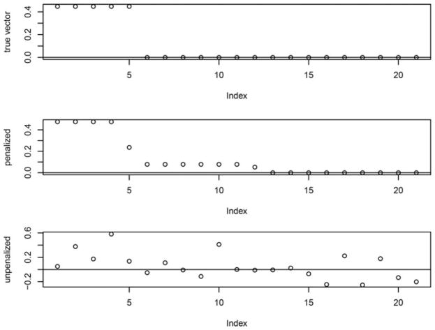
Let α_g and β_g denote the vectors in Eq. (1) that maximize ρ(y^Tα, x^Tβ) with scaling constraints ${\alpha }_g^T{\mathrm{\sum }}_{\mathbf{y}}{\alpha }_g=1$ and ${\beta }_g^T{\mathrm{\sum }}_{\mathbf{x}}{\beta }_g=1$. In the first scenario, let y be a random variable and x be a random vector of length 21 with Σ_y = 2 as the variance of y and Σ_x as the covariance matrix of x, where the ijth element of Σ_x is 2 × 0.3^|i−j|. Let ${\beta }_0=(\text{rep}(1/\sqrt{5},5),\text{rep}(0,16))$, where rep(c, n) represents a sequence of numbers that repeats the number c n times. Then ${\beta }_g={\beta }_0/\sqrt{{\beta }_0^T{\mathrm{\sum }}_{\mathbf{x}}{\beta }_0}$. Since y is a random variable, α_g is a scalar equal to $1/\sqrt{2}$. We let $a_g={\mathrm{\sum }}_y^{1/2}{\alpha }_g$ and $b_g={\mathrm{\sum }}_{\mathbf{x}}^{1/2}{\beta }_g$, and then we let a_g and b_g be the singular vectors from the singular value decomposition of $K={\mathrm{\sum }}_y^{-1/2}{\mathrm{\sum }}_{yx}{\mathrm{\sum }}_x^{-1/2}=a_{g}d{b}_g^T$ with only one nonzero singular value d, set equal to 0.25. Thus, ${\mathrm{\sum }}_{yx}={\mathrm{\sum }}_y^{1/2}{a}_{g}d{b}_g^T{\mathrm{\sum }}_x^{1/2}$. Let the combined random vector of (x, y) follow a multivariate normal distribution with zero means and assembled covariance matrix $\mathrm{\sum }=\left[\begin{array}{ll}{\mathrm{\sum }}_x\hfill & {\mathrm{\sum }}_{xy}\hfill \\ {\mathrm{\sum }}_{yx}\hfill & {\mathrm{\sum }}_y\hfill \end{array}\right]$. We simulated a dataset with sample size n = 300. After normalizing the true and estimated versions of β_g such that ||β_g||₂ = 1, we present the results in Fig. 1. The top panel shows the true β_g, the middle panel shows the result of our method, and the bottom panel shows the result of classical CCA. We can see that when the ratio of the dimension of x to the number of observations is high, our approach yields much better results than those of classical CCA.

Figure 1.

Comparison of leading canonical correlation vectors with the general covariance matrix based on the simulation study.

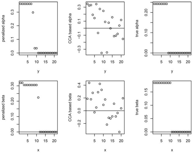
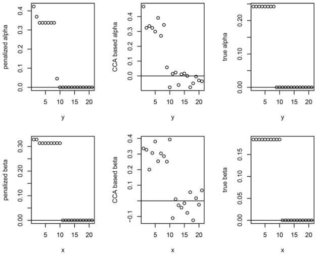
In the second scenario, let x and y be two random vectors of length 21. Let Σ_x and Σ_y be the covariance matrices of x and y, where the ij− element of Σ_x and Σ_y are 2.25 × 0.15^|i−j| and 1.5 × 0.2^|i−j|, respectively. Let ${\alpha }_0=(\text{rep}(1/\sqrt{8},8),\text{rep}(0,13))$ and ${\beta }_0=(\text{rep}(1/\sqrt{10},10),\text{rep}(0,11))$. Then ${\alpha }_g={\alpha }_0/\sqrt{{\alpha }_0^T{\mathrm{\sum }}_{\mathbf{y}}{\alpha }_0}$ and ${\beta }_g={\beta }_0/\sqrt{{\beta }_0^T{\mathrm{\sum }}_{\mathbf{x}}{\beta }_0}$. Let a_g and b_g are also the singular vectors from SVD of $K={\mathrm{\sum }}_{\mathbf{y}}^{-1/2}{\mathrm{\sum }}_{\mathbf{yx}}{\mathrm{\sum }}_{\mathbf{x}}^{-1/2}={\alpha }_{g}D{\beta }_g^T$, where D is a diagonal matrix with the square root of eigenvalues of matrix KK^T as the ith diagonal element. Let d = 0.4 be the only nonzero eigenvalue of KK^T. We have $a_g={\mathrm{\sum }}_{\mathbf{y}}^{1/2}{\alpha }_g$ and $b_g={\mathrm{\sum }}_{\mathbf{x}}^{1/2}{\beta }_g$. Thus, ${\mathrm{\sum }}_{\mathbf{yx}}={\mathrm{\sum }}_{\mathbf{y}}^{1/2}{a}_{g}d{b}_g^T{\mathrm{\sum }}_{\mathbf{x}}^{1/2}$. Let the combined vector of (x, y) follow a multivariate normal distribution with zero means and assembled covariance matrix $\mathrm{\sum }=\left[\begin{array}{ll}{\mathrm{\sum }}_{\mathbf{x}}\hfill & {\mathrm{\sum }}_{\mathbf{xy}}\hfill \\ {\mathrm{\sum }}_{\mathbf{yx}}\hfill & {\mathrm{\sum }}_{\mathbf{y}}\hfill \end{array}\right]$. We first simulated a dataset with sample size n = 300. After normalizing the true and estimated versions of α_g and β_g such that ||α_g||₂ = 1 and ||β_g||₂ = 1, we present the results in Fig. 2. The left panels show the results of our method, the middle panel of classical CCA, and the right panel shows the true values. To explore the behavior of our method with increasing sample size, we next simulated a dataset with 3,000 observations, and the results are shown in Fig. 3. We observe that as the sample size increases, the results based on our method converge to the true ones faster those of classical CCA.

Figure 2.

Comparison of leading canonical correlation vectors with the general covariance matrix n = 300 based on the simulation study.

Figure 3.

Comparison of leading canonical correlation vectors with the general covariance matrix n = 3, 000 based on the simulation study.

In both simulation studies, our method generated estimates close to the true values even with a small sample size, while classical CCA method proved unreliable. With the R package glmnet, the computing and programming is straightforward.

5. Analysis of the WHAT-IF trial

For the WHAT-IF trial analysis, let Y_ij denote the PEth test value of individual i at the jth visit. Let X_ij = (X_ij,1, X_ij,2, …, X_ij,21)^T denote the self-reported daily SDUs during the past 21 days before the PEth test of individual i at jth visit. Let Z_i denote the BMI of individual i with Z_i = 1 if BMI > 25, otherwise Z_i = 0. Let X_ij * Z_i denote the interaction terms between daily SDUs and BMI of individual i at jth visit. To maximize the correlation between PEth and the linear combination of the self-reported daily alcohol intake, we further assume the vector of coefficients in the linear combination can be represented by a step function taking jumps at times when the correlation largely decreases. Since the sample size is limited compared to the number of coefficients we want to estimate, we apply our SCCA method. We also tried to find a vector of coefficients β_par such that the partial correlation between PEth and the linear combination of daily SDUs is maximized given BMI. We assign different penalty factors to X_ij and X_ij * Z_i to distinguish the effects, and we leave Z_i unpenalized.

We first applied our method using the baseline data only. In Fig. 4, the results based on our method are compared to the ones obtained from the classical CCA method after both are normalized to have L² -norm equal to 1. The results of β_par for the penalized partial correlation analysis versus unpenalized are shown in Fig. 5. In both models, the results indicated that PEth is correlated with the previous 12 days alcohol drinking before the test. The results also showed higher influence for the previous 5 days, and a largely reduced influence from day 6 to 12. The results from the penalized partial correlation showed that coefficients of X_i1 * Z_i are zero.

Figure 4.

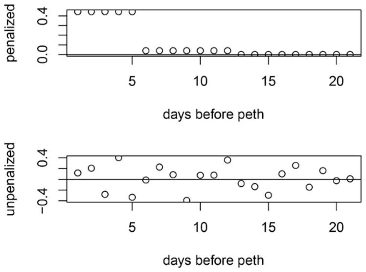
Results based on the lasso penalty vs. ordinary CCA at baseline using the What-If data.

Figure 5.

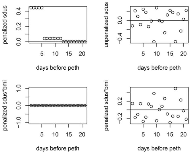
Results of partial correlation given BMI vs. unpenalized at baseline using the What-If data.

Second, we applied our method to the complete data using our method for repeated measures. The results based on our method with all observations are shown in Fig. 6, where we also show the results from the classical CCA method. The results of β_par for the penalized partial correlation analysis are shown in Fig. 7. In both the full and partial correlation cases, the results indicated that PEth is correlated with self-report for 5 days before the test, which is similar to what we observed with the baseline data. Again, the results from the penalized partial correlation showed that coefficients of X_ij * Z_i are zero.

Figure 6.

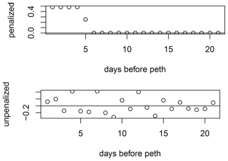
Results based on the lasso penalty vs. ordinary CCA with all observations using the What-If data.

Figure 7.

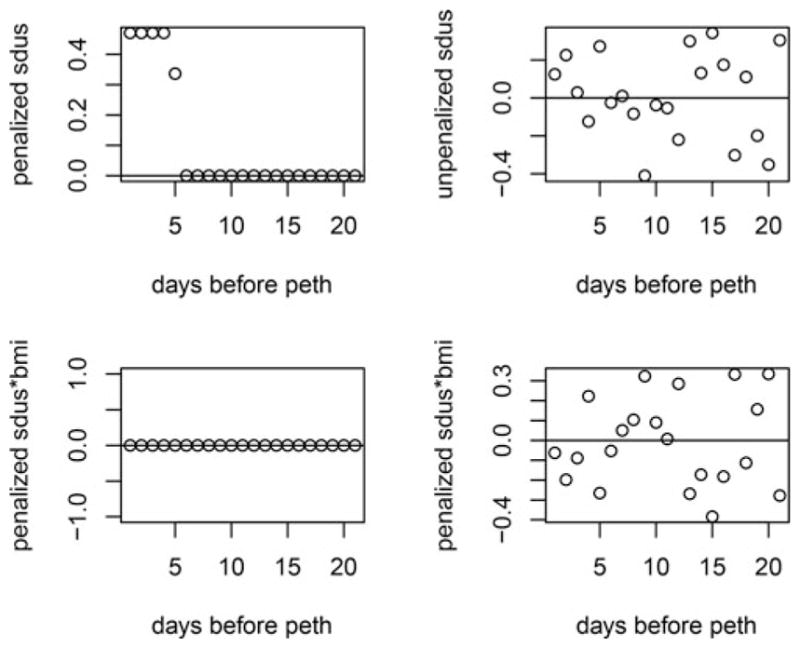
Results of partial correlation given BMI vs. unpenalized with all observations using the What-If data.

Furthermore, to construct confidence intervals, we used both the bootstrap and the jackknife variance estimators. For the bootstrap, we resampled 1,000 times with 120 individuals in each sample. The estimated penalized and unpenalized correlations between PEth and linear combination of daily SDUs with bootstrap and jackknife confidence intervals are listed in Tables 1 and 2. The results of the penalized and unpenalized partial correlation are listed in Tables 3 and 4. Both bootstrap and jackknife confidence intervals based on the complete data showed that the correlation and partial correlation given BMI between PEth and self-report is significant.

Table 1.

Estimated canonical correlation and bootstrap confidence intervals.

	pencor	pc_lower	pc_upper	unpencor	unpc_lower	unpc_upper
Baseline	0.2168	−0.0812	0.5148	0.4492	0.2753	0.6231
All	0.1710	0.0175	0.3245	0.2758	0.1490	0.4026

Table 2.

Estimated canonical correlation and jackknife confidence intervals.

	pencor	pc_lower	pc_upper	unpencor	unpc_lower	unpc_upper
Baseline	0.2168	−0.1143	0.5479	0.4492	0.2675	0.6309
All	0.1710	0.0725	0.2695	0.2758	0.1713	0.3803

Table 3.

Estimated partial canonical correlation with bootstrap confidence intervals.

	pencor	pc_lower	pc_upper	unpencor	unpc_lower	unpc_upper
Baseline	0.2012	−0.2056	0.6080	0.6071	0.4805	0.7337
All	0.1564	0.0240	0.2888	0.4827	0.3954	0.5700

Table 4.

Estimated partial canonical correlation with jackknife confidence intervals.

	pencor	pc_lower	pc_upper	unpencor	unpc_lower	unpc_upper
Baseline	0.2012	−0.0768	0.4792	0.6071	0.1625	1.0517
All	0.1564	0.1157	0.1970	0.4827	0.4562	0.5092

6. Discussion

As part of our case study, we developed a new and easily implemented approach to SCCA by iteratively fitting linear models with a Lasso penalty and a parameterization that favors step functions with just a few downward steps. This led us to conclude that PEth is most strongly correlated with self-report measured over the previous 5 days. We reviewed the relevant literature, and we discovered that the method of Witten and Tibshirani (2009) solves an optimization problem with constraints that change at each iteration. We provided a theoretical grounding for the method of Waaijenborg et al. (2008), which is similar to our method. We showed that when y is a scalar, the two methods coincide and both solve a well-defined optimization problem. When y is a vector, we showed that our method, like that of Witten and Tibshirani (2009), solves an optimization problem with constraints that change at each iteration. Furthermore, we adapted our method to accommodate repeated measures and partial correlation.

We conducted two sets of simulations, first with y as a scalar and second with y as a vector, to validate our methodology. The results showed that our methods perform well in both settings. With the R package glmnet (Friedman et al., 2010), the computation is straightforward.

Appendix: Proofs

A.1. Proof of Theorem 3.1

Let y be a random variable, x be a vector of random variables. Let Var(x) = Σ is nonsingular and Var(y) = σ² < ∞. Then we can always write

$$y={\beta }_0+{\mathbf{x}}^{\mathbf{T}}{\beta }^{\ast }+\epsilon ,$$

where E(ε) = 0, E(ε²) < ∞, Cov(x_j, ε) = 0 for j = 1, …, K, and

$$\begin{gathered} {\beta }^{\ast }={\mathrm{\sum }}^{-1}\text{Cov}(\mathbf{x},y) \\ {\beta }_0=E(y)-E{(\mathbf{x})}^T\beta . \end{gathered}$$

Furthermore, β^* = argmin_βE(y − β₀ − x^Tβ)².

By definition

$$\rho (y,{\mathbf{x}}^T\beta )=\frac{1}{\sigma }\frac{{\beta }^T\mathrm{\sum }{\beta }^{\ast }}{\sqrt{{\beta }^T\mathrm{\sum }\beta }}.$$

Let β^** = Σ^1/2β, then

$$\rho (y,{\mathbf{x}}^T\beta )=\frac{1}{\sigma }\frac{{\beta }^{\ast \ast T}({\mathrm{\sum }}^{1/2}{\beta }^{\ast })}{\sqrt{{\beta }^{\ast \ast T}{\beta }^{\ast \ast }}}.$$

To maximize ρ(y, x^Tβ), we have Σ^1/2β^* = cβ^**, where c > 0 is a scalar, because due to Cauchy Schwarz, max_aa^Tb/||a||₂ is equal to cb for any scalar c > 0. Under the restriction β^TΣβ = β^*TΣβ^*, we have

$${\beta }^{\ast \ast T}{\beta }^{\ast \ast }=c^2{\beta }^{\ast \ast T}{\beta }^{\ast \ast }.$$

Thus, c = 1 and Σ^1/2β = Σ^1/2β^*, then β^* = β_C.

Next, we show that when Var(x) = Σ is singular, the set of β^* that minimize (3.2) is identical to the set of β_C that maximize (3.3), and that ${\beta }^{\ast T}\text{Var}(\mathbf{x}){\beta }^{\ast }={\beta }_C^T\text{Var}(\mathbf{x}){\beta }_C$ is constant over that set.

We write Σ = UDU^T using the spectral decomposition, where U = [U_s, U_n] and D is block diagonal with the first block D_s a diagonal matrix of the nonzero eigenvalues and the second block equal to the zero matrix. Therefore, $\mathrm{\sum }=U_s{D}_s{U}_s^T$ and $U_s^T{U}_n=0$. Let $x_s=U_s^{T}x$ and $x_n=U_n^{T}x$. Then Var(x_s) = D_s and Var(x_n) = 0. From Theorem 3.1, we can write

$$y=E(y)-E{(x_s)}^T{\beta }_s^{\ast }+x_s^T{\beta }_s^{\ast }+\epsilon ,$$

where ${\beta }_s^{\ast }=D_s^{-1}\text{Cov}(x_s,y)$, and where ε is uncorrelated with the elements of x_s. Because Var(x_n) = 0, $x_n^T{\beta }_n$ is constant for any β_n, so we can write

$$y=E(y)-E{(x_s)}^T{\beta }_s^{\ast }-E{(x_n)}^T{\beta }_n+x_s^T{\beta }_s^{\ast }+x_n^T{\beta }_n+\epsilon ,$$

where ε is uncorrelated with the elements of x_s and x_n. Letting β₀ = E(y) − E(x_s)^Tβ_s − E(x_n)^Tβ_n, and defining β such that $x^T\beta =x_s^T{\beta }_s+x_n^T{\beta }_n$, we have that ${\beta }_s^{\ast }=\text{argmin}({\beta }_s)E{(y-{\beta }_0-x^T\beta )}^2$, where β₀ and β are functions of β_s and β_n, and we define ${\beta }^{\ast }={({\beta }_s^T,{\beta }_n^T)}^T$. Note that, whereas ${\beta }_s^{\ast }$ is unique, β^* is a set of values indexed by β_n. Turning our attention to ρ(y, x^Tβ) = ρ(y, x^TU_sβ_s + x^TU_nβ_n) = ρ(y, x^TU_sβ_s) (because x^TU_n is constant), we that have for a given β_n, ${\beta }_{s,C}=\text{argmax}({\beta }_s)\rho (y,x^T\beta )=D_s^{-1}\text{Cov}(x_s,y)\times c$ for any positive scalar c. We can define c so that this ${\beta }_{s,C}={\beta }_s^{\ast }$, and this occurs when ${\beta }_{s,C}^T{D}_s{\beta }_{s,C}={\beta }_s^{\ast T}{D}_s{\beta }_s^{\ast }$. Letting ${\beta }_C={({\beta }_{s,C}^T,{\beta }_n)}^T$ for any β_n, we also have that ${\beta }_C^T\mathrm{\sum }{\beta }_C={\beta }^{\ast T}\mathrm{\sum }{\beta }^{\ast }$. Therefore, the set of β^* that minimize (3.2) is identical to the set of β_C that maximize (3.3), and both sets are indexed by β_n.

A.2. Proof of Theorem 3.2

Let y be a random variable, x be a vector of random variables such that E(y) = μ_y, E(x) = μ_x, Var(x) = Σ is nonsingular and Var(y) = σ² < ∞. Then we can always write

$$y={\beta }_0+{\mathbf{x}}^{\mathbf{T}}{\beta }^{\ast }+\epsilon ,$$

where E(ε) = 0, E(ε²) < ∞, Cov(x_j, ε) = 0 for j = 1, …, K, and

$$\begin{gathered} {\beta }^{\ast }={\mathrm{\sum }}^{-1}\text{Cov}(\mathbf{x},y) \\ {\beta }_0=E(y)-E{(\mathbf{x})}^T{\beta }^{\ast }. \end{gathered}$$

Consider the following optimization problems

$${\beta }_L={\text{argmin}}_{\beta }E{(y-{\beta }_0-{\mathbf{x}}^T\beta )}^2\text{subject}\text{to}{\Vert \beta \Vert }_1\le t$$

and

$${\beta }_C={\text{argmax}}_{\beta }\rho (y,{\mathbf{x}}^T\beta )\text{subject}\text{to}{\beta }^T\text{Var}(\mathbf{x})\beta ={{\beta }_L}^T\text{Var}(\mathbf{x}){\beta }_L,{\Vert \beta \Vert }_1\le t.$$

For the first optimization problem, we have

$$\begin{gathered} E[{(y-{\beta }_0-{\mathbf{x}}^T\beta )}^2]=E{[y-{\mu }_y-({\mathbf{x}}^T-{\mu }_{\mathbf{x}}^T)\beta ]}^2 \\ =E{[y-{\mu }_y-({\mathbf{x}}^T-{\mu }_{\mathbf{x}}^T){\beta }^{\ast }]}^2+{({\beta }^{\ast }-\beta )}^T\mathrm{\sum }({\beta }^{\ast }-\beta ), \end{gathered}$$

and we are solving for β_L such that

$${\beta }_L={\text{argmin}}_{\beta }{({\beta }^{\ast }-\beta )}^T\mathrm{\sum }({\beta }^{\ast }-\beta )\text{subject}\text{to}{\Vert \beta \Vert }_1\le t.$$

Rewrite the criterion with Lagrange multiplier

$${({\beta }^{\ast }-\beta )}^T\mathrm{\sum }({\beta }^{\ast }-\beta )+{\lambda }_1{\Vert \beta \Vert }_1.$$

Take derivative with respect to β, set the equation equals to 0, solve for β with KKT conditions:

$$\begin{gathered} -2\mathrm{\sum }({\beta }^{\ast }-\beta )+{\lambda }_1\mathrm{\Gamma }=0 \\ {\Vert \beta \Vert }_1\le t \\ {\lambda }_1({\Vert \beta \Vert }_1-t)=0 \\ {\lambda }_1\ge 0, \end{gathered}$$

where Γ_i = sign(β_i) if β_i ≠ 0; otherwise, Γ_i ∈ [−1, 1]. let S denote the soft thresholding operator such that S(a, c) = sign(a)(|a| − c)₊, where c ≥ 0 and (x)₊ is defined to equal x if x > 0 and 0 if x ≤ 0. Thus, we have

$$\mathrm{\sum }{\beta }_L=\mathrm{\sum }{\beta }^{\ast }-\frac{{\lambda }_1}{2}\mathrm{\Gamma }=S(\mathrm{\sum }{\beta }^{\ast },\frac{{\lambda }_1}{2}),$$

where if ||β^*||₁ ≤ t then choose λ₁ = 0; otherwise, choose λ₁ such that ||β||₁ = t.

The second optimization problem is equivalent to

$${\beta }_C={\text{argmin}}_{\beta }-{\beta }^{T}a\text{subject}\text{to}{\beta }^T\mathrm{\sum }\beta \le {{\beta }_L}^T\mathrm{\sum }{\beta }_L,{\Vert \beta \Vert }_1\le t$$

where $a=\frac{\mathrm{\sum }{\beta }^{\ast }}{\sigma \sqrt{{\beta }_L^T\mathrm{\sum }{\beta }_L}}$ and the objective function is minimized when β^TΣβ = β_L^TΣβ_L.

Rewrite the criterion with Lagrange multiplier

$$-{\beta }^{T}a+\mathrm{\Delta }{\beta }^T\mathrm{\sum }\beta +{\lambda }_2{\Vert \beta \Vert }_1.$$

Take derivative on β, set the equation equals to 0 and by Karush–Kuhn–Tucker conditions, solve for β:

$$\begin{gathered} -a+2\mathrm{\Delta }\mathrm{\sum }\beta +{\lambda }_2\mathrm{\Gamma }=0 \\ \mathrm{\Delta }({\beta }^T\mathrm{\sum }\beta -{{\beta }_L}^T\mathrm{\sum }{\beta }_L)=0 \\ {\beta }^T\mathrm{\sum }\beta \le {{\beta }_L}^T\mathrm{\sum }{\beta }_L \\ \mathrm{\Delta }\ge 0 \\ {\Vert \beta \Vert }_1\le t \\ {\lambda }_2({\Vert \beta \Vert }_1-t)=0 \\ {\lambda }_2\ge 0. \end{gathered}$$

Then, we have

$$\mathrm{\sum }{\beta }_C=\frac{\text{sign}(\mathrm{\sum }{\beta }^{\ast }){(\mid \mathrm{\sum }{\beta }^{\ast }\mid -{\lambda }_2\sigma \sqrt{{\beta }_L\mathrm{\sum }{\beta }_L})}_{+}}{2\mathrm{\Delta }\sigma \sqrt{{\beta }_L\mathrm{\sum }{\beta }_L}}.$$

Choose Δ such that β^TΣβ = β_L^TΣβ_L. Then we have

$$\mathrm{\sum }{\beta }_C=\frac{\text{sign}(\mathrm{\sum }{\beta }^{\ast }){(\mid \mathrm{\sum }{\beta }^{\ast }\mid -{\lambda }_2\sigma \sqrt{{\beta }_L\mathrm{\sum }{\beta }_L})}_{+}\sqrt{{\beta }_L\mathrm{\sum }{\beta }_L}}{{\Vert \text{sign}(\mathrm{\sum }{\beta }^{\ast }){(\mid \mathrm{\sum }{\beta }^{\ast }\mid -{\lambda }_2\sigma \sqrt{{\beta }_L\mathrm{\sum }{\beta }_L})}_{+}\Vert }_2},$$

where if ||β^*||₁ ≤ t then choose λ₂ = 0; otherwise, choose ${\lambda }_2=\frac{{\lambda }_1}{2}\frac{1}{\sigma \sqrt{{\beta }_L\mathrm{\sum }{\beta }_L}}$, which from the preceding optimization implies that ||β_C||₁ = t.

Thus, β_L = β_C.

When Σ is singular, we can extend this result in much the same way as we extended Theorem 3.1, noting that the inverse of Σ does not appear in the proof of Theorem 3.2. The same kind of argument as for extending Theorem 3.1 can be used to show that β_L and β_C solve the same optimization problems, but that neither will generally be unique. Writing β_L = U_sLβ_sL + U_nLβ_nL and β_C = U_sCβ_sC + U_nCβ_nC, we find that both solve

$$D_s{\beta }_s=D_s{\beta }_s^{\ast }-\frac{{\lambda }_1}{2}\mathrm{\Gamma }=S(D_s{\beta }_s^{\ast },\frac{{\lambda }_1}{2}),$$

where if ||β^*||₁ ≤ t then λ₁ = 0; otherwise, choose λ₁ such that ||U_sβ_s + U_nβ_n||₁ = t. For large t, there will be a set of optima with a unique ${\beta }_s^{\ast }$ accompanied by an arbitrary β_n, as with Theorem 3.1. However for t such that ||β^*||₁ > t, we need to jointly select λ₁, β_n, and β_s s.t. ||β||₁ = t.

References

- Aradottir S, Asanovska G, Gjerss S, Hansson P, Alling C. Phosphatidylethanol (peth) concentrations in blood are correlated to reported alcohol intake in alcohol-dependent patients. Alcohol and Alcoholism. 2006;41:431–437. doi: 10.1093/alcalc/agl027. [DOI] [PubMed] [Google Scholar]
- Boyd S, Vandenberghe L. Convex Optimization. Cambridge UK: Cambridge University Press; 2004. [Google Scholar]
- Breiman L. Better subset regression using the nonnegative garrote. Technometrics. 1995;37:373–384. [Google Scholar]
- Fan J, Li R. Variable selection via nonconcave penalized likelihood and its oracle properties. Journal of the American Statistical Association. 2001;96:1348–1360. [Google Scholar]
- Friedman J, Hastie T, Tibshirani R. Regularization paths for generalized linear models via coordinate descent. Journal of Statistical Software. 2010;33:1–22. [PMC free article] [PubMed] [Google Scholar]
- Hahn JA, Dobkin LM, Mayanja B, Emenyonu NI, Kigozi IM, Shiboski S, Bangsberg DR, Gnann H, Weinmann W, Wurst FM. Phosphatidylethanol (peth) as a biomarker of alcohol consumption in HIV-positive patients in sub-saharan Africa. Alcoholism: Clinical and Experimental Research. 2012;36:854–862. doi: 10.1111/j.1530-0277.2011.01669.x. [DOI] [PMC free article] [PubMed] [Google Scholar]
- Helander A, Péter O, Zheng Y. Monitoring of the alcohol biomarkers peth, cdt and etg/ets in an outpatient treatment setting. Alcohol and Alcoholism. 2012;47:552–557. doi: 10.1093/alcalc/ags065. [DOI] [PubMed] [Google Scholar]
- Jain J, Evans JL, Briceño A, Page K, Hahn JA. Comparison of phosphatidylethanol results to self-reported alcohol consumption among young injection drug users. Alcohol and Alcoholism. 2014;49:520–524. doi: 10.1093/alcalc/agu037. [DOI] [PMC free article] [PubMed] [Google Scholar]
- Kechagias S, Dernroth DN, Blomgren A, Hansson T, Isaksson A, Walther L, Kronstrand R, Kågedal B, Nystrom FH. Phosphatidylethanol compared with other blood tests as a biomarker of moderate alcohol consumption in healthy volunteers: A prospective randomized study. Alcohol and Alcoholism. 2015;50:399–406. doi: 10.1093/alcalc/agv038. [DOI] [PubMed] [Google Scholar]
- Leurgans SE, Moyeed RA, Silverman BW. Canonical correlation analysis when the data are curves. Journal of the Royal Statistical Society, Series B. 1993;55:725–740. [Google Scholar]
- Mardia KV, Kent JT, Bibby JM. Multivariate Analysis. London: Academic Press; 1979. [Google Scholar]
- Parkhomenko E, Tritchler D, Beyene J. Genome-wide sparse canonical correlation of gene expression with genotypes. BMC Proceedings. 2007;1(Supp 1):S119. doi: 10.1186/1753-6561-1-s1-s119. [DOI] [PMC free article] [PubMed] [Google Scholar]
- Parkhomenko E, Tritchler D, Beyene J. Sparse canonical correlation analysis with application to genomic data integration. Statistical Applications in Genetics and Molecular Biology. 2009;8:1–34. doi: 10.2202/1544-6115.1406. [DOI] [PubMed] [Google Scholar]
- Silverman B, Ramsay J. Functional Data Analysis. New York: Springer; 2005. [Google Scholar]
- Stewart SH, Reuben A, Brzezinski WA, Koch DG, Basile J, Randall PK, Miller PM. Preliminary evaluation of phosphatidylethanol and alcohol consumption in patients with liver disease and hypertension. Alcohol and Alcoholism. 2009;44:464–467. doi: 10.1093/alcalc/agp039. [DOI] [PMC free article] [PubMed] [Google Scholar]
- Tibshirani R. Regression shrinkage and selection via the lasso. Journal of the Royal Statistical Society, Series B. 1996;58:267–288. [Google Scholar]
- Viel G, Boscolo-Berto R, Cecchetto G, Fais P, Nalesso A, Ferrara SD. Phosphatidylethanol in blood as a marker of chronic alcohol use: A systematic review and meta-analysis. International Journal of Molecular Sciences. 2012;13:14788–14812. doi: 10.3390/ijms131114788. [DOI] [PMC free article] [PubMed] [Google Scholar]
- Vinod HD. Canonical ridge and econometrics of joint production. Journal of Econometrics. 1976;4:147–166. [Google Scholar]
- Waaijenborg S, Verselewel de Witt Hamer PC, Zwinderman AH. Quantifying the association between gene expressions and dna-markers bypenalized canonical correlation analysis. Statistical Applications in Genetics and Molecular Biology. 2008;7(1):1–27. doi: 10.2202/1544-6115.1329. [DOI] [PubMed] [Google Scholar]
- Wiesel A, Kliger M, Hero AO., III A greedy approach to sparse canonical correlation analysis. 2008 Available at: http://arxiv.org/abs/0801.2748.
- Witten DM, Tibshirani R, Hastie T. A penalized matrix decomposition, with applications to sparse principal components and canonical correlation analysis. Biostatistics. 2009;10:515–534. doi: 10.1093/biostatistics/kxp008. [DOI] [PMC free article] [PubMed] [Google Scholar]
- Witten DM, Tibshirani RJ. Extensions of sparse canonical correlation analysis with applications to genomic data. Statistical Applications in Genetics and Molecular Biology. 2009;8:1–27. doi: 10.2202/1544-6115.1470. [DOI] [PMC free article] [PubMed] [Google Scholar]
- Wooldridge JM. Econometric Analysis of Cross Section and Panel Data. Cambridge, MA: MIT Press; 2010. [Google Scholar]
- Zhou J, He X. Dimension reduction based on constrained canonical correlation and variable filtering. Annals of Statistics. 2008;36:1649–1668. [Google Scholar]
- Zou H, Hastie T. Regularization and variable selection via the elastic net. Journal of the Royal Statistical Society, Series B. 2005;67:301–320. [Google Scholar]