flowLearn: fast and precise identification and quality checking of cell populations in flow cytometry

Abstract

Motivation

Identification of cell populations in flow cytometry is a critical part of the analysis and lays the groundwork for many applications and research discovery. The current paradigm of manual analysis is time consuming and subjective. A common goal of users is to replace manual analysis with automated methods that replicate their results. Supervised tools provide the best performance in such a use case, however they require fine parameterization to obtain the best results. Hence, there is a strong need for methods that are fast to setup, accurate and interpretable.

Results

flowLearn is a semi-supervised approach for the quality-checked identification of cell populations. Using a very small number of manually gated samples, through density alignments it is able to predict gates on other samples with high accuracy and speed. On two state-of-the-art datasets, our tool achieves $\text{median}(F_1)$-measures exceeding 0.99 for 31%, and 0.90 for 80% of all analyzed populations. Furthermore, users can directly interpret and adjust automated gates on new sample files to iteratively improve the initial training.

Availability and implementation

FlowLearn is available as an R package on https://github.com/mlux86/flowLearn. Evaluation data is publicly available online. Details can be found in the Supplementary Material.

Supplementary information

Supplementary data are available at Bioinformatics online.

1 Introduction

Flow cytometry (FCM) is a technology that is commonly used for the rapid characterization of cells of the immune system at the single cell level based on antigens presented on the cell surface. Cells of interest are targeted by a set of fluorochrome-conjugated antibodies (markers) and pass through a laser beam one-by-one at over 10 000 cells per minute (Shapiro, 2005). Scattered light of different wavelengths for each marker is measured and recorded by sensitive detectors. This subsequently creates a unique intensity profile that allows for differentiation of cell types. FCM is widely used in research, for example in immunophenotyping where it holds great promise for assessing the immune status of patient populations. Within a blood or tissue sample, the most common measurement of interest is cell frequency (i.e. the proportion of a cell population), either absolute or relative to a parent population. Variations in cell frequencies can give important information about the immune status or allow association of cell types with a biological variable (Aghaeepour et al., 2016).

The accurate determination of cell population frequencies is a key aim in FCM analysis. Using differential expression of one or more markers, it is possible to delineate cell populations of interest, a process commonly known as ‘gating’. This task usually comprises the manual inspection of bivariate density plots using marker channels that were selected from prior biological knowledge. Subsequently, for each sample, cell populations are identified by drawing regions of interest or setting channel thresholds (Fig. 1). While some populations are easy to gate, populations with very small cell proportions (rare populations) can be challenging. Large populations can obscure rare ones, such that they do not necessarily appear as clusters or well pronounced density peaks, hence are difficult to detect. Due to the large number of possible combinations of markers, gating is a labour intensive and highly subjective process (Saeys et al., 2016). In contrast, automated methods offer little to no bias and comparable variability (Aghaeepour et al., 2013; Finak et al., 2016). Thus, there has been substantial interest in developing methods that ease the process of identifying cell populations as much as possible, and a large variety of tools, both unsupervised and supervised, have been developed (Aghaeepour et al., 2013; Kvistborg et al., 2015; Saeys et al., 2016).

Fig. 1.

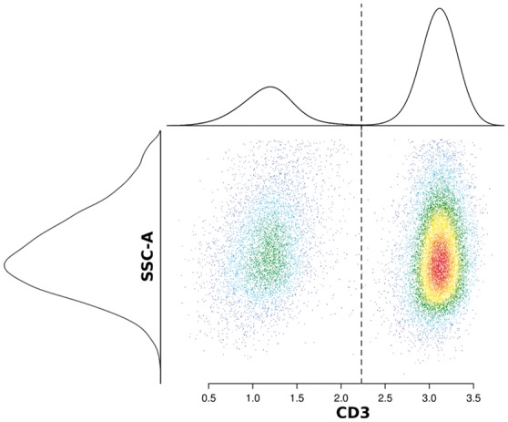
Density plot for two channels ‘CD-3’ against ‘SSC-A’. Each dot represents a cell and corresponding one-dimensional densities are attached at the top and left. The shown data is an example of gating T-cells from lymphocyte singlet cells. Axis values correspond to intensity values. Knowing that T-cells (right cluster) express CD3, they can be delineated from other lymphocytes (left cluster). The corresponding density estimates for both channels are shown along the left and top axis. The CD3 threshold is located in a valley between the density peaks from both populations

Several tools are based on sophisticated techniques from machine learning, i.e. dimensionality reduction, clustering and deep learning. They aim to eliminate the traditional approach of inspecting bivariate channels plots by considering all channels at once instead of only two at a time. While these methods have shown very good performance on many datasets (Amir et al., 2013; Eulenberg et al., 2017; Hennig et al., 2017; Mair et al., 2016), they still suffer from a few major drawbacks, especially pronounced for large sets of highly diverse FCM samples. First, in high-dimensional spaces, cells do not necessarily form distinct clusters that would be easily discoverable. Exemplary, Supplementary Figure S2 shows the t-SNE (Van Der Maaten, 2014) representation of data from Section 3.1. It is visible that both child populations are not distinct from each other. Consequently, for an approach solely based on this technology, it is highly difficult to gate both complex populations. Second, in order to describe populations of interest, the fine-tuning of a set of hyper-parameters is crucial and common to all tools, in particular in the context of small populations where the underlying machine learning task is quite challenging. Hyper-parameters are values controlling the result of an automated method, typically set by practitioners in a way that the outcome of the method is satisfactory. Often, hyper-parameters do not have an intuitive meaning, but relate to mathematical or algorithmic characteristics of the method. Depending on the method, practitioners might not have the required knowledge to set those optimally (Kvistborg et al., 2015). In the presence of high sample diversity, fine-tuning such parameters is essential and might take a significant amount of time. Due to the difficulties in finding an optimal set of parameters, it is also complicated to compare such tools. Third, when incorporating machine learning, interpretability of results is limited (Lisboa, 2013), leading to a lack of general understanding of how such methods work. Hence, it is problematic to verify gates from a biological standpoint (Kvistborg et al., 2015).

In FCM studies, quality checking of results is an essential step in the accurate identification of populations, and ensures that no wrong conclusions are drawn from the data in later steps. For that reason, and also because of the familiarity with the traditional approach of inspecting bivariate density plots, for quality checking, manual gating is the current standard practice.

FlowDensity (Malek et al., 2015) takes another point of view and tries to automate the threshold selection based on density shape features. The algorithm can work in both an unsupervised or supervised fashion. When customizing thresholds on a per-population level, one or more channels are inspected, and density features such as differences in extrema, slope changes, or the number of peaks are examined, generally based on a pre-determined manual gating hierarchy. Gates in the form of channel thresholds are estimated, from which sub-populations can be extracted (Fig. 1). Provided hyper-parameters are appropriately chosen, flowDensity offers a state-of-the-art tool for the accurate identification of cell populations that matches what would have been obtained through manual analysis (Finak et al., 2016). Once the rules for each population are set, thresholds are automatically and individually set for each new data file, similar to the manual tweaking that operators tend to do, but in a data-driven fashion. As a result, flowDensity results are robust, reproducible and the approach performs better than the manual alternative it is designed to match. However, undertaking a supervised setup does require a significant time component in order to obtain the optimal results.

In this contribution, we present a novel software tool called ‘flowLearn’. Using density features, it works the same way as flowDensity, but does not require a practitioner to manually tune hyper-parameters for an optimized outcome. Rather, it works in a semi-supervised mode, and requires the gating of one or few characteristic samples by a human expert in the form of thresholds. These thresholds are then transferred to all samples in an automated way by means of so called derivative-based density alignments. In contrast to methods with a high-dimensional understanding of FCM data, our method does not have to deal with the problem of noise inherent to such spaces. It reduces the problem complexity by relying on traditional, prior biological knowledge. Besides this highly efficient and effective mode, it also opens the way towards a quality control of samples which have already been gated: By comparing optimal and predicted gates, it can identify samples that stand out, for example due to biological variation or differences in laboratory sample preparation and analysis. Furthermore, it can be used to spot problems in existing gating hierarchies, offering the possibility to be used to identify problematic gates. The absence of difficult-to-set hyper-parameters, combined with the use of a small amount of example gates makes our approach tractable. Results are easy to interpret and verify, and offer user-interactive adjustments on the predicted gates in specific circumstances. Using two large and diverse datasets for which accurately set and verified gates exist, and by comparing to two other recent state-of-the-art methods, DeepCyTOF (Li et al., 2017) and FlowSOM (Van Gassen et al., 2015), we demonstrate flowLearn’s superiority for the classical and practically very relevant setting of comparably low dimensional data and imbalanced populations. It exhibits high to very high accuracy in terms of predicted cell frequencies and F₁-measures of identified populations, having low computational complexity.

2 Materials and methods

2.1 Pipeline

FlowLearn is based on four main steps that are depicted in Figure 2. In the following, we will describe these steps in more detail. A more detailed procedure on how to apply flowLearn to a set of samples and populations is given by Algorithm 1.

Fig. 2.

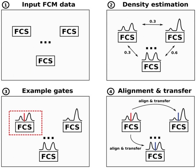
FlowLearn pipeline to gate one population in four consecutive steps: (1) Input to our tool is a set of related FCS files (samples). (2) On each sample, it solves the task of extracting sub-populations from a given parent-population. To achieve this, marker channel densities of the desired population are calculated and a pairwise comparison of all densities is performed. (3) Based on the resulting distances, one or more prototype(s) (red) are selected, for which manual gating is performed. (4) Each prototype density is aligned to all other densities which makes it possible to predict thresholds by transfer between the aligned densities (blue) (Color version of this figure is available at Bioinformatics online.)

1: Input FCM data

We define a dataset $S=\{s_1,s_2,\dots ,s_N\}$ as a collection of N related samples generated using the same panel of antibodies. Each sample contains a set of cells with marker-based measurements of fluorescent intensities, and any subset is called a population. In the following, we assume a population with M cells, and each cell has measurements in the form of marker intensities. We define a marker channel for sample s_i as the set $C_i=\{c_i^1,\dots ,c_i^M\}$ of marker intensity measurements for all M cells. The set of marker channels is experiment-specific, and used across all samples. Furthermore, a sample-specific channel threshold t_i splits up a given channel into two distinct sub-populations $C_{i_1}$ and $C_{i_2}$, such that $C_i=C_{i_1}\cup C_{i_2}$ and $C_{i_1}\cap C_{i_2}=\varnothing$. A gate is defined by a set of thresholds for one or more channels and can delineate sub-populations from a given parent population. Last, a gating hierarchy is the consecutive extraction of sub-populations, starting with one root population that usually contains all cells in the FCS file. It is assumed that the gating hierarchy for a dataset is known, meaning that for each parent population, the set of channels to gate is given.

2: Density estimation

Given a parent cell population, from which sub-populations should be gated, for each sample and channel to gate, flowLearn uses kernel density estimation to generate a unique density profile over a regular grid of 512 points (Algorithm 1, lines 4–9). It uses a Gaussian kernel with a bandwidth determined by Silverman’s rule of thumb (Silverman, 1986). To avoid difficulties in later alignments (step 4), the calculated densities are smoothed by fitting a cubic spline function. In the following, a density for channel C_i is denoted as $d_i=g(C_i)$, where g estimates and smoothes a density from a given channel and parent population in sample s_i. In the resulting distributions, pronounced cell populations are visible as density peaks (Fig. 1). All further processing is done on the N densities for each channel only. For clustering in the next step, pairwise L₁ distances between all densities are calculated as well.

3: Example gates

The alignment (step 4) of two channel densities can be inaccurate if they are very different from each other. In that case, thresholds might be transferred wrongly. To prevent this, flowLearn selects prototypes that define sample groups (Algorithm 1, line 12). Parameterized with the number of prototypes n_p, it clusters all densities for each channel and selects n_p samples that represent each set accurately. We found that for this task, a k-medoids clustering (Friedman et al., 2001) with k = n_p worked best. In this approach, similar densities are characterized by their absolute difference (L₁ distance). Experiments using other distances for clustering, for example the alignment distance, showed worse results. The number of prototypes should be chosen according to the sample diversity in the dataset, and desired gating accuracy. While often n_p = 1 shows very good results (Section 4), with increasing complexity, n_p should be increased accordingly. It is worth to note that, first, n_p can be different for different channels, depending on the data complexity, and second, prototypes for different channels are not necessarily from the same sample.

Next, having the prototypes identified, it is the task of an expert analyst to set gates as accurate as possible, resulting in prototype thresholds (Algorithm 1, line 13). A gate that delineates two populations can be given by lower and upper thresholds for at least one channel. In Figure 1, the T-cell population (right cluster) is defined by a lower threshold on the CD3 channel, meaning that all cells with higher CD3 intensity belong to the target population. The CD3 threshold is located in a valley between the density peaks from both populations. If necessary, an upper threshold can be set as well, even though it is not necessary in this particular example. Also, here the SSC-A channel is irrelevant for gating. A gate can be defined by more than one channel, where two channels are usually chosen for the ease of visualization and interpretability. A limitation is that prototype thresholds have to be perpendicular to the channel axes, though current efforts are focused on addressing this.

Algorithm 1 Applying flowLearn to gate all populations in a given set of FCS files: First, densities are calculated once for all channels. Second, prototype densities are identified and manually gated. Third, all other densities are aligned to the prototypes and thresholds are transferred. This is repeated for each population of interest, starting with all cells.

Input: set of N FCS files, gating hierarchy H

1: $parentPopulation\leftarrow$ all cells

2: $childPopulation\leftarrow$ next in H

3: while not all populations in H gated do

4:  for all FCS files s_ido ▹ Calculate densities once

5:    $Z_i\leftarrow$ cells matching parentPopulation in s_i

6:    for all channels jdo

7:     $d_i^j\leftarrow$ density on j-th channel for cells in Z_i

8:    end for

9:  end for

10:  for all considered channels jdo▹ Predict thresholds

11:    $D_j\leftarrow$ distances between all densities $d_i^j,\hspace{0.17em}\forall$ samples i

12:    $P_j\leftarrow$n_p prototype densities, w.r.t. D_j

13:    let expert set reference threshold(s) on each density in P_j

14:    for all non-prototype densities mdo

15:     $p\leftarrow$ nearest prototype w.r.t. D_j

16:     $a\leftarrow$ DDTW alignment between m and p

17:     transfer reference threshold(s) from p to m using a

18:    end for

19:  end for

20:  gate childPopulation using reference and predicted thresholds

21:  $parentPopulation\leftarrow childPopulation$

22:  $childPopulation\leftarrow$ next in H

23: end while

4: Alignment and gate transfer

Given a prototype sample with density d_p, a known prototype threshold t_p, and another sample’s density d_i, flowLearn is a function $f(d_i,d_p,t_p)={\widehat{t}}_i\approx t_i$, where t_i is the unknown true threshold in d_i. FlowLearn (Algorithm 1, lines 14–18) uses density alignment, Derivative Dynamic Time Warping (DDTW) (Keogh and Pazzani, 2001) in particular. Illustrated in Figure 3, each point in the red-dashed prototype density d_p is matched with a point in the solid-black test density d_i. This makes it possible to transfer the known thresholds t_p to predicted thresholds ${\widehat{t}}_i$. The resulting threshold prediction on the right contains both t_i (red) and ${\widehat{t}}_i$ (blue) with a nearly perfect match. In contrast to regular Dynamic Time Warping, DDTW does not compare absolute density values, but uses local derivatives instead. This way, DDTW puts more focus on aligning shapes. More specifically, because of differences in the size of cell populations, the associated density peaks can locally differ in height, which constitutes a problem for regular DTW: because it only compares absolute height values, local differences make it difficult to align the corresponding density regions (Keogh and Pazzani, 2001). This effect can be remedied by considering derivatives instead. In the case of aligning FCM densities, this is the preferred way, because thresholds are mostly characterized by density features such as extrema or slope changes (Malek et al., 2015). Using flowLearn, it is also possible to gate rare populations by the alignment of density tails. Additional information is shown in Supplementary Figure S6. The idea of alignment has already been proposed in the technology dubbed per-channel basis normalization (Hahne et al., 2010). Here, specific density landmarks are identified and aligned. By using parameter-less shape matching for arbitrary shapes, flowLearn improves on this. In particular, it can take into account rare populations, which are not easily captured by using parameterized density models as in per-channel basis normalization.

Fig. 3.

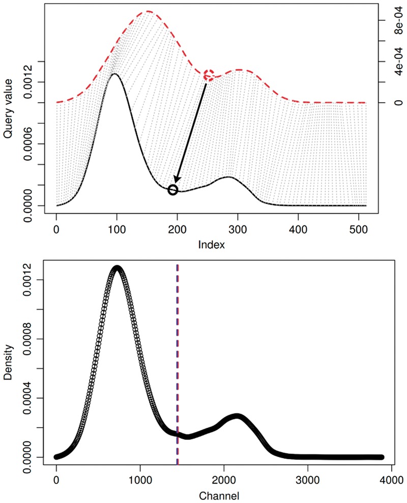
Example of how thresholds are transferred using DDTW alignments. Top: The red-dashed prototype density d_p is aligned to the solid-black test density d_i. The transfer of threshold location is indicated by an arrow. Bottom: Test density d_i with predicted (blue) and true (red) thresholds, ${\widehat{t}}_i$ and t_i, respectively. Both thresholds match up well (Color version of this figure is available at Bioinformatics online.)

2.2 Evaluation measures

We evaluate our method by assessing its performance per predicted population: For that task, we use two measures. First we calculate difference percentages in median cell frequencies $d_f=\frac{\text{median}\left|f_i-{\widehat{f}}_i\right|}{\text{median}\hspace{0.17em}\hspace{0.17em}{f}_i}$ where, for each sample i, f_i and ${\widehat{f}}_i$ are cell frequencies of a given population with regard to the ground truth and predicted gates, respectively. Second, we calculated F₁-measures for all ground truth and predicted populations: Given one sample and population, for one or more channels, true and predicted thresholds, t_i and ${\widehat{t}}_i$, define a gate. Furthermore, a sub-population is defined by all cells that fall within the gate, i.e. have larger/smaller density than the lower/upper threshold for each involved channel. For the sub-population, the true and predicted set of cells, S and $\widehat{S}$, are known. Then the performance on this particular population and sample is defined by $F_1=2·\frac{\text{precision}·\text{recall}}{\text{precision}+\text{recall}}$, where precision and recall are calculated in terms of S and $\widehat{S}$. While analysts are mostly interested in the accuracy of cell frequencies, using the F₁-score for evaluation provides an additional, more informative measure. It is worth to note, that even though thresholds might differ significantly, the agreement of population memberships as measured by the F₁-score can still be high. This is the case when thresholds differ in regions with only a low number of cells.

2.3 Quality checking cell population thresholds

Thresholds might be predicted wrongly either because of sample diversity (i.e. failed alignments with too different prototypes), or because of gates that were set wrongly in the first place. The prediction capabilities and evaluation measures of flowLearn can alternatively be used as a tool for detecting such irregularities in a given set of samples and already existing gates. Samples with deviant F₁-scores can be an indication of unexpected biological variation, differences in reagent preparation and analysis, or wrongly set thresholds. Our method give clues to an expert to further analyze identified, possibly problematic samples or gates. Given an input dataset with existing gates in the form of channel thresholds, quality checking is performed as follows. Similar to Algorithm 1, for each analyzed population:

1. Use flowLearn to identify n_p prototype densities.

2. Let flowLearn gate all other non-prototype samples.

3. Compare predicted populations with ones defined by existing gates.

4. Samples with significant deviation from the average F₁-score suggest problems or give hint to unexpected biological variation.

FlowLearn provides the functionality to identify such outlier samples. Considering the distribution of F₁-scores in a given population, it uses the rule of thumb (Upton and Cook, 1996) that outliers are given by samples with $F_1<Q_1-1.5·\text{IQR}$, where Q₁ is the 25%-quantile and $\text{IQR}$ is the inter-quartile-range of the distribution of F₁-values.

2.4 Implementation and computational complexity

FlowLearn is available as an R-package. By default, using the density function, flowLearn uses a smoothed Gaussian kernel density estimate with a granularity of G = 512 points. This setting is a good compromise between speed and accuracy: For coarse densities, the alignment is fast, however prediction accuracy will suffer. The subsequent spline fitting is performed using R’s smooth.spline function. For prototype selection, the function pam of the package cluster is used. Furthermore, we use the dtw package for alignment and a robust estimate (Keogh and Pazzani, 2001) of derivative $d_i^{deriv}=\frac{\left(d_i-d_{i-1}\right)+\left(d_{i+1}-d_{i-1}\right)/2}{2}$. FlowLearn provides separate methods to identify prototype densities and to predict other samples from there. This way, it can be integrated into existing analysis pipelines.

Computational time complexity of the gating of one population can be broken down into multiple steps. First, density calculation and spline fitting (Algorithm 1, lines 4–9) is performed in $\mathcal{O}(N·(M+G\hspace{0.17em}\text{log}\hspace{0.17em}G))$ and $\mathcal{O}(N·G)$, respectively. The distance matrix calculation and subsequent prototype selection (Algorithm 1, lines 11–12) is done in $\mathcal{O}(N^2)$. By using warping window constraints, DDTW takes place in $\mathcal{O}(N·G)$. Consequently, flowLearn has quadratic time and memory complexity, however practical requirements are very low (Section 4.3).

3 Study design and evaluation datasets

To demonstrate flowLearn’s capabilities to accurately identify populations on a large number of samples, we evaluated it on two distinct datasets (Mice, FlowCAP). Both datasets were used in real-world applications, contain diverse samples, and were augmented with carefully set gates in the form of channel thresholds. For each sample and cell population in both datasets, flowLearn identified n_p prototypes, and predicted gates on the remaining test samples using only the prototypes as a reference. For each population, median cell frequencies and F₁-scores are reported to assess flowLearn’s performance on these data. Furthermore, we compared our results on the Mice dataset with two recent state-of-the-art gating tools for identifying cell populations, DeepCyTOF (Li et al., 2017) and FlowSOM (Van Gassen et al., 2015).

3.1 Mice data

As part of a large study to identify gene-immunophenotype associations in mice (Brown and Moore, 2012), 2665 FCS files from mice bone marrow samples (experiment details given in Supplementary Table S1) were gated, first manually and then using flowDensity, and independently verified. By looking at the variability of resulting cell proportions, the flowDensity gates were found to be superior to manual gates. Hence, flowDensity gates were used as the gold standard for this study. In the following experiments, we refer to these curated thresholds as true gates. The mean cell frequencies of 16 cell populations (relative to the parent population) range from 0.2 to 50%, covering a wide biological diversity, including very rare populations.

3.2 FlowCAP data

We evaluated flowLearn on a second dataset from the FlowCAP (Flow Cytometry: Critical Assessment of Population Identification Methods) consortium (Finak et al., 2016). FlowCAP provides the means to objectively test methods for the identification of cell populations, and puts out state-of-the-art datasets with which it is possible to compare tools to manual analysis by experts. In the context of the FlowCAP-III competition, seven participating centers were given the task to analyze three samples. For each sample, three replicates were analyzed, and for each replicate, sub-populations in four datasets [B cells, T cells, Regulatory T cells (T-reg), Dendritic Cells (DC)] were identified independently from each center. Manual gating was performed by a central site. For each dataset, a total of 63 FCS files were available for evaluation. Since flowLearn currently uses channel thresholds, we used only populations with rectangular gates, 54 in total. Mean cell frequencies (relative to the parent population) range from 0.4 to $70\%$. Even though, all centers were advised to follow reagent and analysis standardization, technical variation between centers was still large (Finak et al., 2016), leading to a greater sample diversity in this dataset. This effect is also pronounced in the densities estimated by flowLearn, i.e. the sample diversity is captured in the densities as well. For illustration, we used t-SNE (Van Der Maaten, 2014) to project densities to two dimensions. In Supplementary Figure S1 it is visible that within-center densities are more similar to each other than to other centers, indicating between-center variability.

4 Results

4.1 Mice data

For each population of the Mice dataset (2665 samples of clean CD45 bone marrow cells), we gated a small number of $n_p\in \{1,2,5,10,50\}$ prototypes (using flowDensity and manual curation). These thresholds were transferred to all samples by the described flowLearn protocol. We refer to those thresholds as the predicted ones. Figure 4 shows the result of n_p = 1, where results on all 2664 test samples per population are represented by boxplots. Distributions of true and predicted cell frequencies match up well, with $\text{mean}\hspace{0.17em}\hspace{0.17em}{d}_f=0.05$ ($\min d_f=0.0001$, $\max d_f=0.22$), taken over all populations. Additionally, in Supplementary Figures S33 and S34, it is visible that errors of both predicted thresholds and cell frequencies are concentrated near zero for all datasets. Also, predicted gates are accurate with respect to extracted cell populations, specifically we have $\text{median}(F_1)>0.99$ for the majority (9/16) of populations and $\text{median}(F_1)>0.90$ for the large majority (15/16). Rare populations such as T cells (4% of parent) and Plasma cells (0.2% of parent) show high performance. The CD43 population’s low variability could not be matched (Supplementary Section S5). For some populations, a minority of samples with lower F₁-scores exist, including outliers (represented as dots) with poor F₁-score. Choosing the number of prototypes $n_p>1$ increases performance significantly, especially for populations with initially low performance (Supplementary Figs S8–S12). For the HFC population, choosing n_p = 10 increases the result to $\text{median}(F_1)=0.94$.

Fig. 4.

Results on the Mice dataset using one prototype. Left: True and predicted cell frequencies for each population. Right: F₁-scores for each population (2665 samples). Outliers are shown as single dots. Populations HFA to HFF stand for Hardy-Fraction A to F (explained in Supplementary Table S3). Populations denoted with an asterisk are non-biological (technical) populations

4.2 FlowCAP data

On the FlowCAP data, we ran flowLearn using $n_p\in \{1,4,7,11,20\}$ prototype(s). As the dataset contained only 63 samples, we chose n_p = 7 prototypes (i.e. one prototype per center). Table 1 shows a statistic for difference percentages in cell frequencies for all datasets. The average differences were low, ranging from 5 to 14 percent. While for some populations, differences were negligible, for other populations, differences were large. Furthermore, a summary of F₁-scores is shown in Figure 5, where the minimum and average population $\text{median}(F_1)$-scores, depending on n_p is displayed for each dataset. Performance depended on both the population and more strongly on the chosen number of prototypes. Considering all datasets, for n_p = 7 (number of centers), 20/64 populations achieve $\text{median}(F_1)>0.99$ and $\text{median}(F_1)>0.90$ for 51/64 populations. Results on other populations are not as good when only few prototypes ($n_p<7$) are chosen, and are generally not as good as on the Mice dataset. In general, choosing more prototypes yields higher F₁ values. Especially for populations that perform poorly, increasing n_p significantly increases performance. Results for all datasets can be found in the Supplementary Material (Supplementary Figs S13–S32).

Table 1.

For each dataset, minimum, average and maximum difference percentages in cell frequencies

	Mice	DC	T-cells	T-reg	B-cells
np	1	7	7	7	7
$\min d_f$	0.0001	0.01	0.001	0.001	0.002
$\text{mean}\hspace{0.17em}\hspace{0.17em}{d}_f$	0.05	0.11	0.13	0.14	0.08
$\max d_f$	0.22	0.62	0.13	0.14	0.22

Fig. 5.

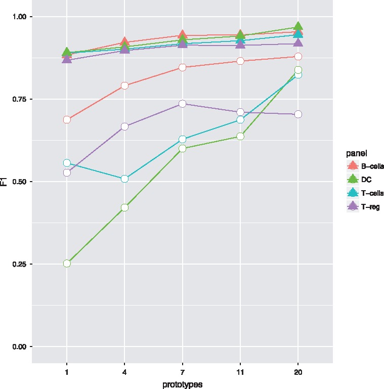
Results on the FlowCAP dataset, with minimum (circle) and mean (triangle) population performances for all four datasets, depending on the chosen number of prototypes

4.3 Runtime

For the Mice data (16 populations), gating and evaluating all 2665 samples using one prototype took one hour (1.3 s per sample). By exploiting parallelism, practical runtimes are low. When using n_p prototypes, flowLearn will perform n_p alignments per sample per population. Increasing n_p also linearly increases runtime. Again, for the Mice data, using n_p = 2 took 62 min (n_p = 10: 66 min, n_p = 50: 111 min). In all experiments, using a Dell M3800 laptop (Intel^® Core^TM i7-4712HQ processor), resident memory usage never exceeded 5 GB of RAM. These results indicate that flowLearn can be run on recent consumer laptops without problems.

4.4 Comparison to DeepCyTOF and FlowSOM

We compared flowLearn to two recent state-of-the-art methods for population identification, DeepCyTOF (Li et al., 2017) and FlowSOM (Van Gassen et al., 2015). DeepCyTOF exhibited very high F₁-scores on multiple datasets, being better than all best-performing methods on data from the FlowCAP-I competition (Aghaeepour et al., 2013). In a recent study (Weber and Robinson, 2016), FlowSOM outperformed 18 competing tools. We ran both methods on the Mice dataset and compared results to the ones obtained by flowLearn (Supplementary Fig. S7). Details on the exact evaluation procedure can be found in Supplementary Table S2. Since these methods return disjoint clusters (only one cluster ID per cell), suitable populations are given by all leaf populations in the gating hierarchy. We evaluated F₁-scores in the same manner as for flowLearn. DeepCyTOF predicted seven out of ten populations with $\text{median}\hspace{0.17em}\hspace{0.17em}{F}_1>0.75$, with $\text{mean}\hspace{0.17em}\hspace{0.17em}{F}_1=0.79$. FlowSOM was able to achieve $\text{median}\hspace{0.17em}\hspace{0.17em}{F}_1>0.75$ for four out of ten considered populations. Other populations were subpar. The FlowSOM average performance over all considered populations and samples, $\text{mean}\hspace{0.17em}\hspace{0.17em}{F}_1=0.53$, is similar to results obtained previously (Weber and Robinson, 2016). Using the same populations, and using n_p = 1 only, flowLearn achieved $\text{mean}\hspace{0.17em}\hspace{0.17em}{F}_1=0.94$, demonstrating flowLearn’s superiority on this data.

Furthermore, we compared runtimes of DeepCyTOF, FlowSOM and flowLearn. On the Mice data, using ten populations, not including the one-time investment for training the deep network, DeepCyTOF was able to classify each sample in an average of one second. Using the same populations, FlowSOM was able to gate one sample in an average of 11 s which is in accordance with results reported in (Van Gassen et al., 2015). On the same data, flowLearn predicted 2664 samples for one population in 1.37 min. For comparability, predicting ten populations with flowLearn takes 13.7 min, 0.31 s per sample. This does not include the time spent for providing manual gates to flowLearn.

5 Discussion

On two state-of-the-art datasets, flowLearn achieves $\text{median}(F_1)$-measures exceeding $F_1>0.99$ for 20/64 (31%), and $F_1>0.90$ for 51/64 (80%) of all analyzed populations. It predicts populations with low bias and variance, using only few examples (Mice: n_p = 1, FlowCAP: n_p = 7). Hence, it is possible to gate very few training files to obtain excellent results for most cell populations for thousands of additional files. However, there are populations, for which it is difficult to predict gates ($F_1<0.9$). We identified possible causes: First, we found that flowLearn can identify possible sample-based irregularities, in particular samples with densities that are significantly different from all other densities in a given dataset. Such differences might exist due to either biological diversity or anomalous sample reagent preparation and analysis. For example, the HFC population of the Mice dataset has many wrongly predicted samples with low F₁-score (Fig. 4). Here, flowLearn identified all samples with $F_1<0.56$ as outliers. In all included box plots, these are shown as individual dots. By visualizing sample densities from that population, and coloring each sample by F₁-score in Figure 6, it is visible that samples with F₁-score below the identified threshold form a distinct region, but not necessarily a separate cluster. Supplementary Figure S3 shows that this observation can be made for only one channel, giving more specific information about the source. Furthermore, a closer look at wrongly predicted HFC samples (Supplementary Fig. S4) explains their poor performance. While in the large majority of samples, the HFC population is very well pronounced, in samples with low F₁-score, it is either completely missing or pronounced only very weakly. This leads to wrongly set thresholds in the training data, or failed DTW alignments. Detecting such irregularities confirms flowLearn’s capabilities of being used as an appropriate tool for quality checking.

Fig. 6.

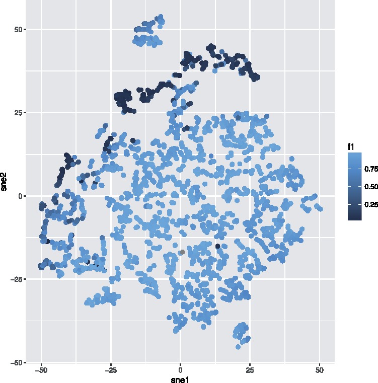
t-SNE projection of Mice densities (HFC population) from one channel, colored by F1-score according to predictions using n_p = 1. Samples with low performance cluster together

Next, we analyzed the sub-optimal performance of some populations in the FlowCAP dataset. Here, all datasets exhibit a wide diversity in terms of samples, centers and gates (Finak et al., 2016). We observed that this variability impacts on the ability of flowLearn to correctly predict gates. An example is shown in Supplementary Figure S5, which shows the same T-cell/CD4 Effector population from two different FCS files and that densities and gates for the displayed channel are very different from each other. Despite the difference in both densities, the alignment looks correct. However, because of the difference in threshold locations, a threshold transfer will incorrectly predict the resulting gate. We observed similar effects on most other low-performing populations from the FlowCAP dataset. Reasons for wrongly predicted gates include differences in thresholds, failed alignments due to large differences in samples, and also few failed alignments even though samples were similar.

To prevent wrong alignments due to large sample differences, flowLearn’s clustering approach is essential and picks prototypes that are representative for all other samples. In some cases (especially in the presence of high sample diversity) it can happen, that a prototype is wrongly aligned to all other samples, resulting in reduced prediction performance. The number of prototypes is important as well. We showed that flowLearn can accurately predict gates using only one prototype, but again, when there is high sample diversity, performance can be improved significantly by using more. The data might come from experiments in which samples can be categorized, for example into healthy/diseased or wild type/knockout, or samples were analyzed in different centers. In such cases where there is prior knowledge about the data, the number of prototypes should be chosen accordingly. Generally, performance depends on the heterogeneity of the observed densities. At present, the number of prototypes is set manually within the pipeline, but this choice could be automated in order to guarantee a sufficient sample homogeneity within every single prototype cluster.

Last, when compared to two recent state-of-the-art methods, DeepCyTOF and FlowSOM, our method showed superior performance in terms of F₁-scores. While all methods aim to solve the same problem of identifying cell populations, it is worth to highlight that depending on the application, one might be better suited than another. FlowSOM has the advantage that it does not require any prior knowledge about the data at hand, in particular no manual gating is needed. Being completely unsupervised, however it is expected that it cannot perform as well as its supervised counterparts. Both DeepCyTOF and FlowSOM can be used for high-dimensional data such as from mass cytometry. In the case of DeepCyTOF, if addressing the difficult problem of automatically finding good hyper-parameters and network architectures (Klein et al., 2016), it may be used for end-to-end machine learning, i.e. directly inferring biological variables from a given set of cells, without gating (Mair et al., 2016). In contrast, flowLearn automates the prevalent paradigm of gating using channel thresholds for lower-dimensional data. This condition gives our tool an advantage over other tools that have to search a much larger function space. At the same time, being based on channel thresholds makes our results interpretable and adjustable, an advantage that is not directly given for other tools. Furthermore, DeepCyTOF and FlowSOM return assignments of disjoint cell populations. In a gating hierarchy, cells can have multiple labels, and assignment with such methods is difficult. Last, it is worth to note that in the right hands, by carefully choosing method parameters, both DeepCyTOF and FlowSOM may yield better results. In contrast, flowLearn’s parameters are robust and tuning is not necessary.

6 Conclusion

We have shown that flowLearn is able to accurately identify FCM cell populations. In a quality checking setting, flowLearn can also be used to identify both anomalous samples and aberrant thresholds from existing gatings. Using simple density alignments, on two diverse datasets it demonstrated good to excellent performance on a wide variety of populations, including very rare ones. This can be achieved using as few as only one gated sample, keeping invested resources for gating at a minimum level. Furthermore, on a large set of bone marrow samples, we have shown that flowLearn is superior to DeepCyTOF and FlowSOM, two top-performing methods according to recent comparisons. On highly diverse FCM samples such as from different datasets or centers, flowLearn shows its limitations, although in general, choosing more prototypes can increase performance significantly. The correct choice of reference densities is essential for prediction. In the future we will investigate more options to choose better prototypes, for example by including alignment properties or using averaged densities instead of the current prototype-based approach. It would also be beneficial to include confidence measures for the suitability of a given prototype, for example based on alignment distances. With that, one could judge the number of needed prototypes as well. Furthermore, we are interested in using alignments of two-dimensional densities, which would enable the usage of arbitrarily shaped gates. We are also working with third-party commercial tool vendors (e.g. FlowJo, FCSExpress) to extract the rotation required to bring thresholds orthogonal to the axis as required for our current implementation. Being based on the R ecosystem, flowLearn is ready to be included into existing FCM analysis pipelines, and offers improvements thereof in terms of gating quality and resource investment.

References

- Aghaeepour N. et al. (2013) Critical assessment of automated flow cytometry data analysis techniques. Nat. Methods, 10, 228–238. [DOI] [PMC free article] [PubMed] [Google Scholar]
- Aghaeepour N. et al. (2016) A benchmark for evaluation of algorithms for identification of cellular correlates of clinical outcomes. Cytometry A, 89, 16–21. [DOI] [PMC free article] [PubMed] [Google Scholar]
- Amir E.D. et al. (2013) viSNE enables visualization of high dimensional single-cell data and reveals phenotypic heterogeneity of leukemia. Nat. Biotechnol., 31, 545–552. [DOI] [PMC free article] [PubMed] [Google Scholar]
- Brown S.D., Moore M.W. (2012) The international mouse phenotyping consortium: past and future perspectives on mouse phenotyping. Mamm. Genome, 23, 632–640. [DOI] [PMC free article] [PubMed] [Google Scholar]
- Eulenberg P. et al. (2017) Reconstructing cell cycle and disease progression using deep learning. Nat. Commun., 8, 463. [DOI] [PMC free article] [PubMed] [Google Scholar]
- Finak G. et al. (2016) Standardizing flow cytometry immunophenotyping analysis from the human immunophenotyping consortium. Sci. Rep., 6, 20686. [DOI] [PMC free article] [PubMed] [Google Scholar]
- Friedman J. et al. (2001). The Elements of Statistical Learning, Vol. 1 Springer Series in Statistics Springer, Berlin. [Google Scholar]
- Hahne F. et al. (2010) Per-channel basis normalization methods for flow cytometry data. Cytometry A, 77, 121–131. [DOI] [PMC free article] [PubMed] [Google Scholar]
- Hennig H. et al. (2017) An open-source solution for advanced imaging flow cytometry data analysis using machine learning. Methods, 112, 201–210. [DOI] [PMC free article] [PubMed] [Google Scholar]
- Keogh E.J., Pazzani M.J. (2001) Derivative dynamic time warping. In: Proceedings of the 2001 SIAM International Conference on Data Mining. SIAM, pp. 1–11.
- Klein A. et al. (2016) Fast bayesian optimization of machine learning hyperparameters on large datasets. Proceedings of Machine Learning Research, 54, 528–536. [Google Scholar]
- Kvistborg P. et al. (2015) Thinking outside the gate: single-cell assessments in multiple dimensions. Immunity, 42, 591.. [DOI] [PMC free article] [PubMed] [Google Scholar]
- Li H. et al. (2017) Gating mass cytometry data by deep learning. Bioinformatics, 33, 3423–3430. [DOI] [PMC free article] [PubMed] [Google Scholar]
- Lisboa P.J. (2013) Interpretability in machine learning—principles and practice In: Masulli F.et al. (eds) International Workshop on Fuzzy Logic and Applications. Springer, Cham, Switzerland, pp. 15–21. [Google Scholar]
- Mair F. et al. (2016) The end of gating? An introduction to automated analysis of high dimensional cytometry data. Eur. J. Immunol., 46, 34–43. [DOI] [PubMed] [Google Scholar]
- Malek M. et al. (2015) flowdensity: reproducing manual gating of flow cytometry data by automated density-based cell population identification. Bioinformatics, 31, 606–607. [DOI] [PMC free article] [PubMed] [Google Scholar]
- Saeys Y. et al. (2016) Computational flow cytometry: helping to make sense of high-dimensional immunology data. Nat. Rev. Immunol., 16, 449–462. [DOI] [PubMed] [Google Scholar]
- Shapiro H.M. (2005) Practical Flow Cytometry. John Wiley & Sons, Hoboken, USA. [Google Scholar]
- Silverman B.W. (1986) Density Estimation for Statistics and Data Analysis, Vol. 26 CRC Press, Boca Raton, USA. [Google Scholar]
- Upton G., Cook I. (1996) Understanding Statistics. Oxford University Press, Oxford, UK. [Google Scholar]
- Van Der Maaten L. (2014) Accelerating t-sne using tree-based algorithms. J. Mach. Learn. Res., 15, 3221–3245. [Google Scholar]
- Van Gassen S. et al. (2015) Flowsom: using self-organizing maps for visualization and interpretation of cytometry data. Cytometry A, 87, 636–645. [DOI] [PubMed] [Google Scholar]
- Weber L.M., Robinson M.D. (2016) Comparison of clustering methods for high-dimensional single-cell flow and mass cytometry data. Cytometry A, 89, 1084–1096. [DOI] [PubMed] [Google Scholar]
Associated Data
This section collects any data citations, data availability statements, or supplementary materials included in this article.